NON-EQUILIBRIUM IONIZATION MODEL FOR STELLAR CLUSTER WINDS AND ITS APPLICATION
Abstract
We have developed a self-consistent physical model for super stellar cluster winds based on combining a 1-D steady-state adiabatic wind solution and a non-equilibrium ionization calculation. Comparing with the case of collisional ionization equilibrium, we find that the non-equilibrium ionization effect is significant in the regime of a high ratio of energy to mass input rate and manifests in a stronger soft X-ray flux in the inner region of the star cluster. Implementing the model in X-ray data analysis softwares (e.g., XSPEC) directly facilitates comparisons with X-ray observations. Physical quantities such as the mass and energy input rates of stellar winds can be estimated by fitting observed X-ray spectra. The fitted parameters may then be compared with independent measurements from other wavelengths. Applying our model to the star cluster NGC 3603, we find that the wind accounts for no more than 50% of the total “diffuse” emission, and the derived mass input rate and terminal velocity are comparable to other empirical estimates. The remaining emission most likely originate from numerous low-mass pre-main-sequence stellar objects.
1 INTRODUCTION
Super star clusters (SSCs) consist of densely-packed massive stars with typical ages of a few Myr. They are the most energetic coeval stellar systems, identified in a wide range of star-forming galaxies (Whitmore, 2000). Within a characteristic radius of a few pc or less, winds from individual stars in such a cluster are expected to collide and merge into a so-called stellar cluster wind. In some extragalactic systems, such as the nuclear region of M82 (Strickland et al., 2002), winds from star clusters, either individually or collectively, can be energetic enough to drive galaxy-scale superwinds. Consequently, cluster winds can play an important role in shaping star formation and galaxy evolution in general (Heckman et al., 1990).
Observationally, X-ray emission that appears to be diffuse has been detected around star clusters (e.g., NGC 3603, Moffat et al. 2002; Arches cluster at the Galactic center, Yusef-Zaden et al. 2002, Rockefeller et al. 2005, Wang et al. 2006). Theoretically, both stellar cluster wind (e.g., Stevens & Hartwell, 2003, and references therein) and galactic superwind (e.g., Strickland & Stevens, 1999; Breitschwerdt & Schmutzler, 1999) have been investigated, particularly in terms of their expected X-ray luminosities. However, neither the observed spectral nor spatial information has been used to confront the theoretical model prediction quantitatively. Furthermore, most models assume collisional ionization equilibrium (CIE) and no non-equilibrium ionization (NEI) model is available for a quantitative comparison with current X-ray data of stellar cluster winds and/or superwinds.
In this paper, we first introduce our non-equilibrium ionization model for stellar cluster winds based on combining a 1-D steady-state adiabatic wind solution (§2) with a non-equilibrium ionization calculation (§3). The non-equilibrium ionization effect is examined within a grid of parameter space, which is described in §4. Then we report its application to the diffuse X-ray emission of NGC 3603 (§5). The physical parameters (e.g., mass input rate, terminal velocity, and metallicity) of the stellar cluster wind are derived from the fits and compared with other independent measurements and empirical estimates.
2 X-RAY EMISSION FROM STELLAR CLUSTER WINDS
On the scale of a galaxy, supernovae in a starburst region can drive a strong wind. Chevalier & Clegg (1985) describe it by an outflow model with uniformly distributed mass and energy depositions within a radius. Their solutions are scalable to the case of a star cluster, in which the mass loading and energy input are due to stellar winds instead of supernovae.
Essentially analogous to the model of Chevalier & Clegg (1985), Cantó, Raga & Rodríguez (2000) present an analytic 1-D model to describe the cluster wind. In addition, their 3-D numerical simulation of stellar winds from 30 stars produces a mean flow that agrees well with their analytic model. They predict that the X-ray emission from the cluster wind of the Arches cluster (see also Raga et al., 2001) is detectable (Law & Yusef-Zadeh, 2004). Also based on the work of Chevalier & Clegg (1985), Stevens & Hartwell (2003, henceforth, SH03) present a model that allows for a lower energy transfer efficiency and mass loading. This model predicts global properties such as the X-ray luminosity and gas temperature at an individual cluster center. A crude comparison of the model predictions and existing Chandra observations does not give any conclusive result as to whether or not the diffuse emission is genuinely associated with cluster winds.
All of the above theoretical models assume CIE for the ionization structure. However, one may suspect that the gas in a cluster wind may be in a highly NEI state, because of both the rapid shock heating in the wind-wind collision and the fast adiabatic cooling in the subsequent expansion. Fig. 1 illustrates such a NEI condition in a cluster wind. Clearly, the dynamic (adiabatic) cooling time scale defined by is much shorter than the recombination time scales of all key ion species, and CIE does not hold.

Moreover, the mass and energy injections in the previous theoretical models are input parameters and are crudely estimated from the properties (e.g., spectral type and radio flux) of individual massive cluster stars. Such a modeling approach suffers significant uncertainties and has little predictive power. Stellar mass loss remains one of the largest uncertainties in stellar evolution (e.g., Kudritzki & Puls, 2000). Massive stars are also not the only sources of mass loss; other cold mass loading, such as outflows from protostars(e.g., SH03), may also be important.
In the following subsections, we introduce our dynamic model of a stellar cluster wind.
2.1 Cluster Wind Dynamics
We consider a young star cluster (age ), from which the main mass and energy injections are due to stellar winds, especially from those massive OB and Wolf-Rayet stars. Extending SH03’s work, which assumes a uniform distribution of stars, we have constructed a 1-D steady-state wind model with (1) either an exponential or uniform distribution of stars; (2) a steady and spherically symmetric cluster wind; (3) mass and energy injections following the stellar mass distribution; (4) gravity and radiative cooling being neglected. This cluster wind can then be described by the following steady-state Euler equations:
| (1) |
| (2) |
| (3) |
where and are the velocity, density and pressure of the flow respectively, and is the adiabatic index, taken as for an ideal gas, while and are the mass and energy input rates per unit volume and are assumed to be proportional to the stellar mass density .
The total mass and energy input rates are and . When the stellar mass distribution is assumed to be uniform, and , where is the cluster radius, which coincides with the sonic radius; the analytic solutions of Eq. (1)-(3) can be found in Chevalier & Clegg (1985). For an exponential stellar mass distribution, , where is the scale radius. We solve the above Euler equations numerically. Because gravity is negligible, the sonic radius depends on the stellar mass distribution alone.
The above hydrodynamical equations do not predict how the electron temperature changes in the cluster. The temperature depends on how the electron is heated. We consider two extreme cases: one that has the electron and ion temperatures in equilibration, i.e., ; the other that sets the initial and lets the ratio evolve via electron-ion Coulomb collisions. Here, the mean temperature and is the mean mass per particle in terms of the proton mass . Assuming cosmic abundances, the variation in the electron temperature follows the equation (e.g., Eq. (1) in Borkowski et al., 1994):
| (4) |
where is the total particle number density.
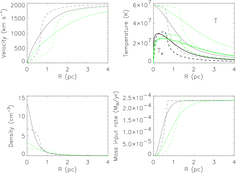
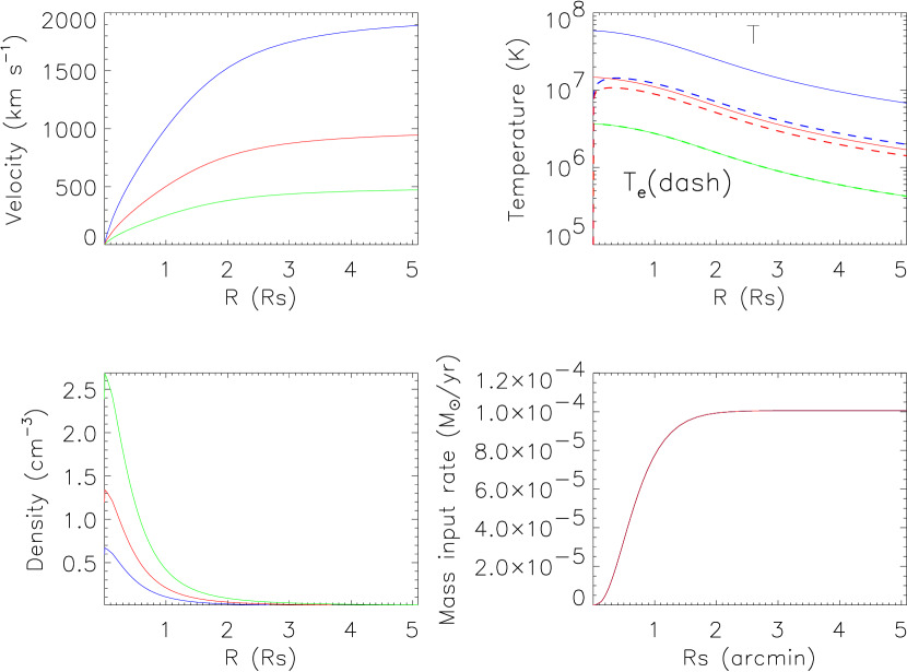
Our model has four parameters: mass input rate , stellar wind terminal velocity (assuming ), abundance Z, and the scale radius (or cluster radius for a uniformly mass distributed model). Fig. 2 illustrates the radial profiles of the mean/electron temperature, density, terminal velocity and mass input rate for these two stellar distribution models with the same sonic radius. Two sonic radii (0.69 pc, black; 1.38 pc, green) are considered here. When the sonic radius is larger, the density is lower in the inner part of the cluster, the temperature drops more slowly, and the terminal velocity of the wind is reached at a larger radius.
2.2 X-ray Emission Calculation
The broad band X-ray luminosity of the cluster wind within a region () is given by:
| (5) |
where is the frequency band of interest; and are the electron and hydrogen number density respectively; is the specific emissivity at frequency , and the cluster wind is assumed to be optically thin. Generally is a function of elemental abundances, local ionic fractions and electron temperature.
The model-predicted spectrum from a given projected annulus between the inner-to-outer radii can be calculated using the following equation:
| (6) |
where is the distance to the cluster. The observed surface brightness can be predicted as:
| (7) |
where and are the on-axis effective area and energy response matrix of the X-ray telescope/instrument.
In principle, both the spatial and spectral information of the data can be used to constrain our model. But while we may reasonably assume the spectrum of the undetectable point sources to be the same as that of detected point sources, a similar assumption about the surface brightness cannot be made because the detected point sources are sparse and incomplete in a typical observation. Therefore, unlike the spectrum, the observed surface brightness cannot easily be compared with the model prediction at present.
3 NON-EQUILIBRIUM IONIZATION SPECTRAL MODEL
In the past, NEI models have been developed for (1) time-dependent isobaric or isochronic cooling of shock-heated gas (e.g., Sutherland & Dopita, 1993), (2) delayed ionization in SNRs (e.g., Borkowski et al., 2001), and (3) delayed recombination in galactic winds (e.g., Breitschwerdt & Schmutzler, 1999) or in the Local Bubble (e.g., Breitschwerdt et al., 1996). The atomic data used are typically more than a decade old and are stored in a way that is difficult to update. Moreover, the physical processes included are not complete, due to either the lack of atomic data or the use of the CIE approximation. One example of such a process is the cascade of electrons following recombinations into highly excited levels, which could strongly affect the line emissivities of highly ionized species (e.g., Gu, 2003).
We have developed a NEI spectral model that has the following characteristics: (1) the ionization code is separated from the atomic data so that the latter can be updated conveniently; (2) the most updated atomic data are used; (3) recombinations into highly excited levels are included; (4) the electron temperature evolution, the dynamics, and the ionization structure are determined self-consistently.
3.1 Atomic Data
Our atomic data are based on CHIANTI (Young et al., 2003, version 4.2), which provides a database of atomic energy levels, transition wavelengths, radiative transition probabilities (A-rates) and electron collisional excitation rates for 23 elements from H () to Zn (), totally 206 ions.
Spectral calculations involving detailed fine structure levels are time-consuming and are not necessary for the current X-ray CCD spectral resolution. Therefore, we have combined those fine structure levels together according to their degeneracies and have re-calculated the collisional excitation rates and A-rates. For example, for the hydrogen ion there are totally 25 energy levels listed in CHIANTI. After regrouping, we get six principle energy levels (1s, 2s, 2p, n=3, n=4 and n=5). For n=3, there are five sub-levels (), which we regroup as one. The new collisional de-excitation rate and A-rate are and respectively, where is the individual sub-level degeneracy and is the total.
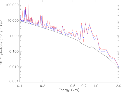
A comparison between CHIANTI and our code with the regrouped data is shown in Fig. 3. The total luminosity difference between the two spectra is less than 1%. The difference in the line structure is very slight at keV and somewhat more noticeable at lower energies. But such difference is well within the uncertainties of the atomic data.
The ionization structure of a plasma is determined by the collisional ionization and radiative and dielectronic recombinations (e.g., Mazzotta et al., 1998, and references therein). CHIANTI does not offer the rates of these atomic processes. We have taken the collisional ionization cross-sections from Arnaud & Rothenflug (1985) and Arnaud & Raymond (1992), and radiative and dielectronic recombination rates from Verner & Ferland (1996) and Mazzotta et al. (1998), except for Carbon, Nitrogen and Oxygen. For these three species, we use the results of Nahar (2000), based on a large-scale close-coupling R-matrix calculation for photoionization cross-sections and recombination coefficients. We assume that three-body recombinations are not important at the density range under consideration and neglect them for all ions. Our current code also does not include charge-exchange reactions.
Fig. 4 compares the CIE ionic fractions of our calculation with those given by Mazzotta et al. (1998, henceforth Mazz98). All, except for C, N, O and Fe, agree well because the same atomic data are used. We find good agreement for all the ions of N, with the difference being less than 10%. For C and O, there is good agreement except for CV, CVI, OIV, OV and OVI, for which the difference can reach up to 50% near the peak of maximum ionic fraction. For example, at , our ionic fraction of OV is a factor of two less than that of Mazz98. From to where ionic fractions of Fe XV to Fe XXI are significant, our calculation is substantially different from Mazz98, particularly for FeXVII to FeXXII. This is due to different radiative recombination rates employed.


3.2 Continuum and Line Emissions
The continuum emission consists of free-free, free-bound and two-photon continua. We include two important two-photon transitions: H-like and He-like .
There are several ways to produce spectral lines in a plasma. Most spectral lines are produced by electron collisional excitation of ions followed by the radiative decay of the excited level. At X-ray energies free electrons can also excite an inner-shell electron to a level above the ionization potential. The excited level of the ion then undergoes either a radiative decay to a lower energy level to produce a satellite line, or an autoionizing transition to the next ionization stage (Dere et al., 2001). We follow CHIANTI in treating this autoionizing transition as a radiative decay to the ground level but with no emission of radiation. In addition, we include the line emission following an inner-shell ionization. For example, an impact ionization from the inner shell of ion contributes to the production of a certain line in the next higher ion . We use the database of Mewe & Cronenschild (1981) for such lines (see Gorczyca et al. (2003) for an assessment of the database accuracy).
Line photons are also produced during the cascade following a radiative recombination into an excited level. This process is particularly important in a delayed recombination scenario. A dielectronic recombination leads to the capture of an incident electron into an excited state above the ionization threshhold of the recombined ion and also emits a photon if an autoionization does not ensue.
3.3 Level Balance Equations
Electron populations at various energy levels of each ion are determined by such processes as collision excitation/de-excitation and radiative decay; the level balance equations are:
| (8) |
where and denote individual levels of an ion, is the total rate of the transitions between the two levels, and is the level population relative to the total level population.
In a low density plasma, collisional excitation generally dominates over recombination in populating the excited states. In an over-cooled NEI state, however, the temperature may be sufficiently low that recombination can make a non-negligible contribution to the level population (e.g., Dere et al., 2001). We include radiative recombinations into the principle energy levels ( to 6) of each ion; the level balance equation for ion (element with electrons removed) is
| (9) |
| (10) |
where is the electron collisional rate, is the radiative decay rate (zero if ), and is the radiative recombination rate to the level of ion . Following Osterbrock (1989), we calculate the rate using Milne’s relation and the photoionization cross sections of Karzas & Latter (1961) for excited states and those of Verner & Yakovlev (1995) for ground states. Thus,
| (11) |
and
| (12) |
where and are the degeneracy and photoionization cross section of level of ion .
3.4 Non-equilibrium Ionization Calculations
In general the dynamics and ionization of a plasma are entangled. The ionization structure, through its heating/cooling effects, can affect the temperature evolution. However, in a cluster wind, radiative cooling can typically be neglected and the dynamics and ionization of the wind can be separated. With the mass input having a certain spatial distribution in our model, and assuming the newly injected gas to be neutral, the cluster wind number density of the neutral ion for a given element evolves in a cluster wind as:
| (13) |
with Z and being the abundance and mass of element .
The number density of other ions () of the same element will follow:
| (14) |
where and are the total ionization () and recombination () rate coefficients (in ) of ion . Our interest here is in highly ionized ions. Therefore, the exact ionization state of the injected gas is not important as long as it is cold or warm (i.e. ).
For each element, we simultaneously solve these differential equations using IDL code LSODE which adaptively solves stiff and non-stiff systems of ordinary differential equations.
In an evolving plasma, a characteristic time scale to approach a CIE state is (Mewe, 1997). The CIE approximation requires the cooling/heating time be much longer than . As mentioned earlier, CIE is only a special case. If experiencing a rapid heating or cooling process such as thermal instability, shock, or rapid expansion, a plasma may be under-ionized or over-ionized, compared to the CIE result (Dopita et al., 2002).
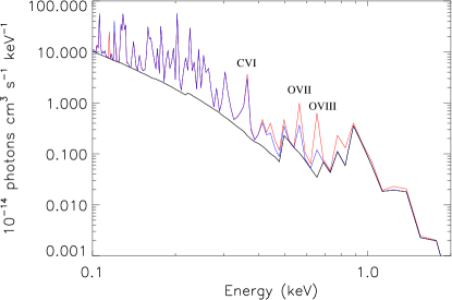
As an illustration, we consider a toy model for an adiabatically expanding stellar cluster wind with a constant mass input rate and a constant velocity . We assume that the wind is injected at an initial radius of pc and is heated up to a CIE state with an equilibrium temperature . As the wind expands adiabatically, its temperature drops as . Fig. 5 compares the CIE and non-CIE spectra at (left panel) and at (right panel). The difference is significant: in the lower energy part, the line intensities in the non-CIE spectrum are weaker than those in the CIE case, while in the upper energy part saw-tooth structures are present in the non-CIE spectra; all these are due to delayed recombinations.
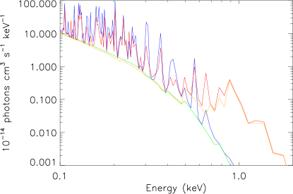
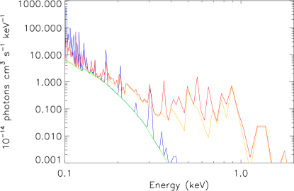
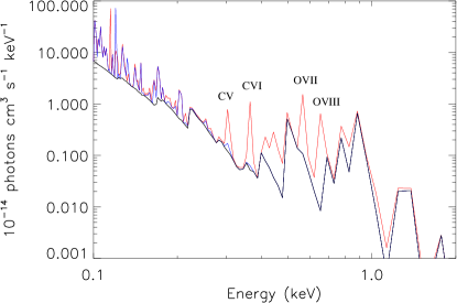
Fig. 6 shows the spectra at the same two radii with and without including the cascade of electrons following recombinations to levels. The cascade lines of CV, CVI, OVII and OVIII are clearly visible.
The more general model for a cluster wind with distributed mass and energy injections has been described in §2.1, and the radial profiles of the wind are shown in Fig. 2. We use the case of , , and a sonic radius pc to illustrate the effect of a distributed mass injection on the ionization structure. Fig. 7 compares the ionic fractions of C, N, O and Fe at four radii between the case in which is all injected at the center and that in which it is injected in an exponential distribution. The effect of the distributed mass injection clearly shows up as a long ionization tail.

4 MODEL PREDICTIONS FOR STELLAR CLUSTER WINDS
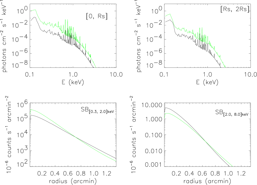
To illustrate the condition under which the NEI effect is significant for stellar cluster winds, we here consider a cluster of an exponential stellar distribution with a scale radius , corresponding to a sonic radius at . We calculate results for a parameter grid: ; . The velocity, temperature, and density profiles of the wind are illustrated in Fig. 8. We consider both the equilibration and non-equilibration cases of the electron and ion temperatures (§2.1) and both the CIE and non-CIE scenarios for comparison. To demonstrate the results, we calculate the intrinsic cumulative spectra for three annular regions, [0, ], [, 2], and [2, 4], as well as the predicted Chandra ASIS-S count intensity distribution over the [0, 2] range and in two energy bands, [0.3, 2.0] keV and [2.0, 8.0] keV. For illustration, we assume that the distance to the cluster is kpc and that the metal abundance is solar.
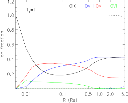
First, we find that the separate evolution does not lead to significant spectral difference in the cumulative spectrum. It is already seen from Fig. 8 that is significantly lower than only when the density is low (i.e. and ). Even in this case the ionic fractions of the key O and Fe ions are fairly similar (Fig. 9). The biggest difference in the ionic fractions between the two evolutions occurs during the rise of from K to K in the non-equilibration evolution (). In the region making the most contribution to the X-ray flux (), the ionic fractions are comparable between the two evolutions in either the CIE or non-CIE case. Henceforth in the following discussions on the cumulative spectrum and count intensity distribution, only the results from the evolution via Coulomb interactions are used.
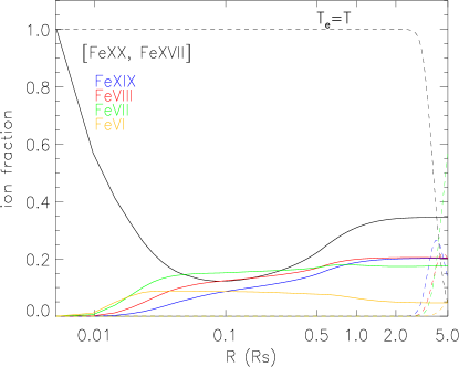
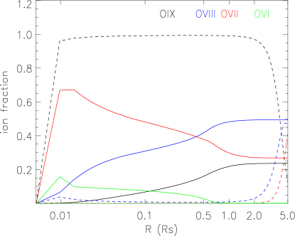
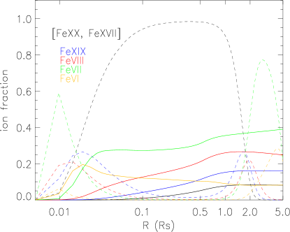
Second, we find that the effect of the NEI manifests itself in both the inner and outer regions of the cluster wind, but under different dynamical conditions. In the inner region it is expected that the CIE and non-CIE calculations will be similar for the cases of high central densities. Fig. 10 illustrates such a case ( and ), in which the CIE approximation is good. Both calculations produce very similar cumulative spectra in either the [0, ] or [, 2] region, although the count intensity distributions can differ by as much as a factor of 2 in either the soft or hard X-ray band. On the other hand, the assumption of CIE in the inner region is poor for and , which leads to a low central density. Fig. 11 shows clearly that the two ionization calculations produce quite different spectra. Also the soft X-ray count intensity from the CIE calculation is an order of magnitude weaker than that from the non-CIE calculation. This discrepancy is due to the difference in the ionic fraction of the two calculations (Fig. 9). The ionization time scale is longer than the dynamical time scale over which the density drops, so O and Fe are not ionized to as high a degree as specified by CIE at the high central temperature. We refer to this contrast as delayed ionization. Fig. 12 shows the spatial dependence of the ionic fraction weighted by pertinent to the calculation of the cumulative spectrum, and compares the CIE and non-CIE spectra at , where the largest contribution to the cumulative spectrum for [0, ] comes from. Clearly, much stronger OVII, OVIII lines and Fe-L complex show up in the non-CIE spectrum. They contribute to the soft X-ray excess seen in Fig. 11.
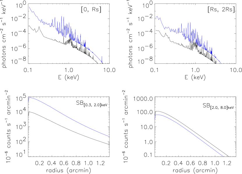
In the outer region, specifically [2, 4], the density has decreased so much from spherical expansion that the CIE assumption is clearly not valid in any of the six wind profiles studied. The contrast between the non-CIE and CIE spectra then depends on how far the temperature drops below , when OIX ions begin to recombine. The more rapidly the temperature decreases with radius, the more the ionization structure deviates from the CIE result. Fig. 13 compares the CIE and non-CIE spectra in the [2 4] region. While the two spectra are quite similar in the case, the non-CIE spectrum in the case clearly produces a stronger hard X-ray flux from a saw-tooth-like recombination continuum. The left panel of Fig. 14 compares Oxygen ionic fractions between CIE and non-CIE calculations. In the outer region (e.g., ), OIX, which produces recombination edges and cascade lines, is absent in the CIE but present in the non-CIE calculation. The right panel of Fig. 14 clearly shows the corresponding spectral differences in the two calculations.
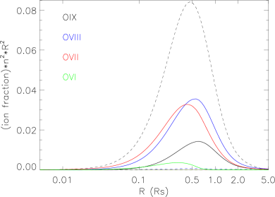
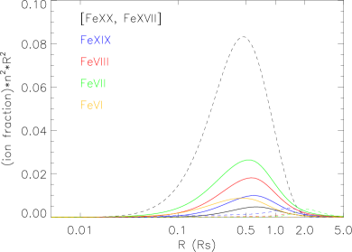
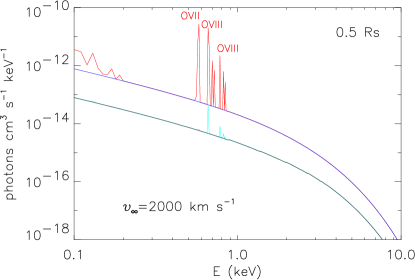
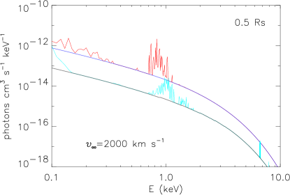
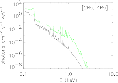
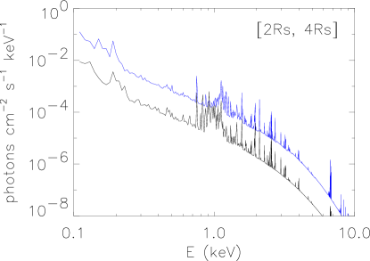
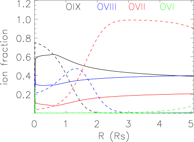
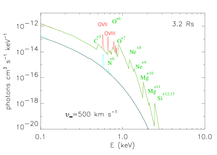
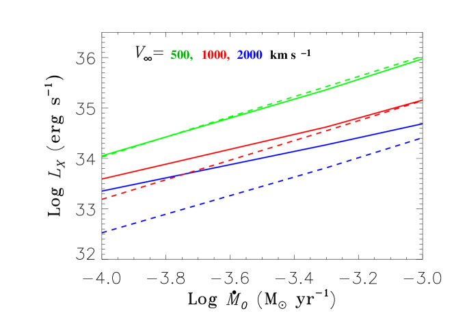
Fig. 15 shows the dependence of the cumulative X-ray luminosity on the mass input rate and wind velocity. The large discrepancy (up to almost one magnitude) between the CIE and non-CIE calculations happens for the high and low combination, i.e., at a high ratio of energy to mass input rate. In addition, the slope dependence is exactly 2 in the CIE calculation in which the cooling function depends only on the local temperature and density. At a fixed , the temperature distribution is insensitive to , so . In the non-CIE case, however, depends on the evolutionary history of the ionization structure; the slope varies from 2 for , in which the CIE approximation is valid, to for .
The above analysis indicates that the ionization structure is intimately related to the dynamical evolution. CIE is a fair approximation only for the case of a low ratio of energy to mass input rate. Some other processes not considered in our model might weaken/strengthen the non-CIE effect for the stellar cluster wind scenario. For example, outflows from protostars present in a cluster can be regarded as a mass loading process. In this case, the total mass input rate and the density will increase. As shown in SH03, the velocity and temperature will decrease instead, which causes a lower ratio of energy to mass input rate.
Our model may also be applied to galactic superwinds. X-ray emission from strong superwinds may be detectable at very larger radii, where delayed recombination becomes important. But in this case, radiative cooling may not be neglected. Theoretical recombination spectrum has been shown in modelling galactic wind/outflow for the local starburst galaxy NGC3079 (Breitschwerdt, 2003).
5 APPLICATION TO NGC 3603
NGC 3603 at a distance of 7 kpc is the most luminous giant HII region in the Galaxy (e.g., Moffat et al., 1994). The star cluster responsible for the HII region is regarded as a Galactic analogue to SSCs observed in other galaxies. With an age of less than (Sung & Bessell, 2004), the cluster contains massive stars as well as low-mass pre-main sequence (PMS) stars.
Stars in NGC 3603 have been investigated from near-infrared to X-ray (e.g., Sung & Bessell, 2004; Moffat et al., 2002). Based on 44 spectroscopically classified stars, which dominate the mass and energy injections, SH03 estimate the total mass input rate from the cluster as and the mean weighted stellar wind terminal velocity as . We use the observed diffuse X-ray emission of NGC 3603 to test our NEI model of stellar cluster winds.
5.1 Data Analysis
We use the Chandra ACIS-I observation of NGC 3603 (observation ID 633), which was taken in May, 2000 for an exposure of 50 ks. Moffat et al. (2002) used this observation to study primarily discrete X-ray sources, although they also characterized the remaining “diffuse” emission with a one-temperature CIE thermal plasma model. Here, we concentrate on the diffuse emission.
We reprocess the ACIS-I event data, using the Chandra Interactive Analysis of Observations software package (CIAO, version 3.2). This reprocess, including the exclusion of time intervals with background flares, results in a net 47.4 ks exposure (live time) for subsequent analysis.
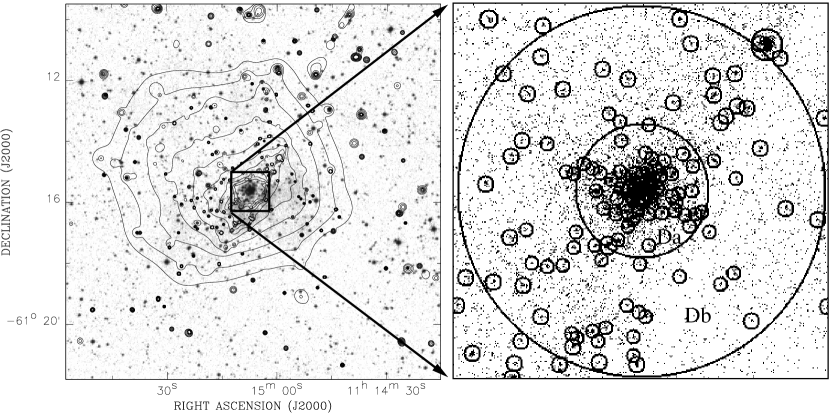
The superb spatial resolution of the data allows for the detection and removal of much of the X-ray contribution from individual stars. We search for X-ray sources in the 0.5-2, 2-8, and 0.5-8 keV bands by using a combination of three source detection and analysis algorithms: wavelet, sliding-box, and maximum likelihood centroid fitting (Wang, 2004). Source count rates are estimated with the 90% energy-encircled radius (EER) of the point spread function (PSF). The accepted sources all have the local false detection probability . The right panel of Fig. 16 shows the detected point sources within the cluster field. The source detection in the inner radius of the cluster is highly incomplete due to severe source confusion.
To analyze the remaining “diffuse” emission from the cluster, we remove the detected source regions from the data. For each faint source with a count rate (CR) , we exclude a region of twice the 90% EER, which increases with off-axis angle. For each source with CR , an additional factor of is multiplied to the source-removal radius to further minimize the residual contribution from the PSF wings of relatively bright sources.
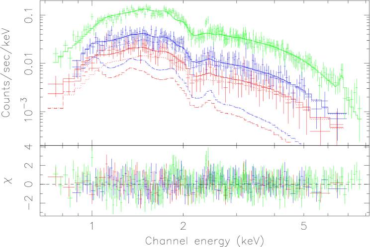
We extract the spectra of the diffuse X-ray emission separately from the two annular regions, Da and Db (divided to contain roughly the same number of counts), as well as an accumulated point source spectrum from the combined region (Da+Db). An additional spectrum extracted from the outer annulus between 40 and 50 radii is used as the local background of the diffuse X-ray emission, which in turn are normalized for the background subtraction of the sources. Fig. 17 shows a joint-fit of the spectra with our cluster wind model plus a thermal model, which is used to characterize the point-like source spectrum. Here we assume that the detected and undetected point sources have the same spectral shape. We jointly fit the diffuse spectra and the accumulative spectrum of point sources together. We find that the spectral fit results are insensitive to the assumed stellar distributions of our model and to the exact scale radius. Therefore, Table 1 includes only the results from the model with the more physical exponential stellar mass distribution; the fixed scale radius corresponds to the same sonic radius as adopted by SH03. The best-fit model predicts the luminosity contributions of and from the cluster wind and residual point-like source components. Fig. 18 shows the predicted radial surface intensity distribution of the cluster wind contributions compared with the observed “diffuse” emission in two energy bands.


| Parameter | Model | |
|---|---|---|
| Cluster wind component | ||
| (pc) | 0.68 (fixed) | |
| Abundance | ||
| () | 1.53 () | |
| Point-like source component | ||
| (keV) | ||
| bb is the MEKAL normalization of the undetected point sources in Region Da. | ( photons cm-2) | |
| cc is same as , but in Region Db. | ( photons cm-2) | |
| dd refers to the MEKAL normalization of the detected point sources. | ( photons cm-2) | |
5.2 Discussion
The above results represent the first quantitative comparison of a self-consistent NEI cluster wind model with observational data. Our fitted foreground X-ray-absorbing gas column density, , is consistent with the interstellar reddening toward NGC 3603. The reddening of , determined by Sung & Bessell (2004) from 115 bright stars in the field, corresponds to (e.g., Bohlin et al., 1978). The derived abundance of the wind is sub-solar: . This abundance likely represents an underestimate of the true value due to the oversimplification in the 1-D model, which does not account for substructures in both temperature and density. Such substructures lead to smearing out of spectral line features that characterize the metal abundance. Our fitted mass input rate and terminal velocity of the cluster wind is, within a factor of , consistent with the empirical estimation by SH03 (§5). But the cluster wind contributes only about 25% of the observed total diffuse emission luminosity.
While the remaining of the diffuse emission likely originate from undetected point-like sources, what is their nature? Moffat et al. (2002) and Sung & Bessell (2004) suggested that PMS young stellar objects (YSOs) may be responsible. According to the study by Saga et al. (2001), the NGC 3603 cluster has an initial mass function (IMF) that can be characterized by a power law with a slope of 0.84 and contains about stars in the mass range 7-75 . Using this IMF, we estimate the presence of about YSOs (0.3-3 ) in this cluster. The study of such YSOs in the Orion Nebular (Feigelson et al., 2005) shows that their average 2-8 keV luminosity is per star. Thus the expected total YSO contribution in the NGC 3603 cluster is , consistent with the prediction from our spectral fit.
6 SUMMARY
In this paper, we have presented a NEI spectral code, which is based on our updated atomic data, including the atomic process of recombinations into highly excited levels. We have shown important differences between the CIE and non-CIE calculations.
We have constructed a self-consistent physical model for super stellar cluster winds, combining the NEI code with a 1-D steady-state adiabatic wind solution. We find that in the inner region of the star cluster, the NEI effect is significant in the regime of a high energy to mass input ratio and manifests in an enhanced soft X-ray emission, which could be an order of magnitude more luminous than that obtained under the CIE assumption.
We apply the cluster wind model to the Chandra data on NGC 3603 and find that the inferred mass and energy input rates of the stellar cluster winds are comparable to the empirical estimates. But the cluster wind in NGC 3603 accounts for no larger than 50% of the total diffuse X-ray emission. YSOs are likely responsible for the remaining diffuse emission.
References
- Allen (1973) Allen, C.W. 1973, Astrophysical Quantities
- Arnaud & Rothenflug (1985) Arnaud, M., & Rothenflug, R. 1985, A&AS, 60, 425
- Arnaud & Raymond (1992) Arnaud, M., & Raymond, J. 1992, ApJ, 398, 394
- Bohlin et al. (1978) Bohlin, R.C., Savage, B.D., & Drake, J.F., 1978, ApJ, 224, 132
- Borkowski et al. (1994) Borkowski, K.J., Sarazin, C.L., & Blondin, J.M. 1994, ApJ, 429, 710
- Borkowski et al. (2001) Borkowski, K.J., Lyerly, W.J., & Reynold, S.P. 2001, ApJ, 548, 820
- Breitschwerdt et al. (1996) Breitschwerdt D., Egger, R., Freyberg, M.J., Frisch, P.C., Vallerga, J.V. 1996, Space Sci. Rev., 78, 183
- Breitschwerdt & Schmutzler (1999) Breitschwerdt D., & Schmutzler, T. 1999, A&A, 347, 650
- Breitschwerdt (2003) Breitschwerdt D. 2003, Rev.Mex.Astron.Astrof.Ser.Conf. 15, 311
- Cantó, Raga & Rodríguez (2000) Cantó J., Raga A. & Rodríguez L. 2000, ApJ, 536,896
- Chevalier & Clegg (1985) Chevalier R, & Clegg A., 1985 Nature, 317, 44
- Dere et al. (2001) Dere, K.P., Landi, E., Young, P.R., DeL Zanna, G. 2001, ApJ, 134, 331
- Dopita et al. (2002) Dopita, M.A., Sutherland, R.S., Schweiger, G.S. 2002, Astrophysics of the Diffuse Universe , Berlin, New York: Springer.
- Feigelson et al. (2005) Feigelson, E.D., Getman, K., Townsley, L., et al. 2005, ApJS, 160, 379
- Gorczyca et al. (2003) Gorczyca, T.W., Kodituwakku, C.N., Korista, K.T., Zatsarinny, O. 2003, ApJ, 592, 636
- Gu (2003) Gu, M.F. 2003, ApJ, 582, 1241
- Heckman et al. (1990) Heckman, T. M., Armus, L., & Miley, G. K. 1990 ApJS, 74, 833
- Kaastral & Mewe (1993) Kaastra, J.S., & Mewe, R. 1993, A&AS, 97, 443
- Karzas & Latter (1961) Karzas, W.J., & Latter, R. 1961, ApJS, 6, 167
- Kudritzki & Puls (2000) Kudritzki, R. & Puls, J. 2000, ARA&A, 38, 613
- Law & Yusef-Zadeh (2004) Law, C., & Yusef-Zadeh, R. 2004, ApJ, 611,858
- Mazzotta et al. (1998) Mazzotta, P., Mazzitelli,G., Colafrancesco S. Vittorio N. 1998, A&AS, 117 , 920 (Mazz98)
- Mewe & Cronenschild (1981) Mewe, R., & Cronenschild, E.H.B.M. 1981, A&AS, 45, 11
- Mewe (1997) Mewe, R. 1997, in X-ray spectroscopy in Astrophysics, eds. J. van Paradijs, Bleeker J.A.M., Lectrure Notes in Physics, 520, 109
- Moffat et al. (1994) Moffat, A.F.J., Drissen, L., & Shara, M.M. 1994, ApJ, 436, 183
- Moffat et al. (2002) Moffat, A.F.J., Corcoran, M.F., Stevens, I.R., et. al 2002, ApJ, 573, 191
- Nahar (2000) Nahar, S.N. in Atomic Data Needs In X-Ray Astronomy, 2000, ed. M.A. Bautista, T.R., Kallman, & A.K. Pradhan (NASA/CP-2000-209968), 75
- Osterbrock (1989) Osterbrock, D.E. 1989, Astrophysics of Gaseous Nebulae and Active Galactic Nuclei
- Raga et al. (2001) Raga A.C., Velázquez, P.F., Cantó J., Masciadri, E. Rodríguez L.F. 2001 ApJ, 559, L33
- Rockefeller et al. (2005) Rockefeller, G., Fryer, C.L., Melia, F., Wang, Q.D. 2005, ApJ, 623, 171
- Saga et al. (2001) Saga, R., Munari, U., de Boer, K.S. 2001, MNRAS, 327, 23
- Stevens & Hartwell (2003) Stevens, I.R., & Hartwell, J.M. 2003 MNRAS, 339, 280 (SH03)
- Strickland & Stevens (1999) Strickland, D.K., & Stevens, I.R. 1999, MNRAS, 306, 43
- Strickland et al. (2002) Strickland, D.K., Heckman, T.M., Weaver, K.A., Hoopes, C.G., & Dahlem, M. 2002, ApJ, 568, 689
- Sung & Bessell (2004) Sung, H., & Bessell, M.S. 2004, AJ, 127, 1014
- Sutherland & Dopita (1993) Sutherland, R.S., & Dopita, M.A. 1993, ApJS, 88, 253
- Verner & Yakovlev (1995) Verner, D.A., & Yakovlev, D.G. 1995, A&AS, 109, 125
- Verner & Ferland (1996) Verner, D.A., & Ferland, G.J. 1996, ApJS, 103, 467
- Wang (2004) Wang, Q.D. 2004, ApJ, 612, 159
- Wang et al. (2006 ) Wang, Q.D., Dong, H., & Lang, C. C. 2006, MNRAS, submitted
- Whitmore (2000) Whitmore, B. 2000, STScI Symposium Series 14, ed. M. Livio, astro-ph/0012546
- Young et al. (2003) Young, P.R., Del Zanna, G., Landi, E., Dere, K. P., Mason, H. E., & Landini, M. 2003, ApJS, 144, 135
- Yusef-Zaden et al. (2002) Yusef-Zadeh, F., Law, C., Wardle, M., Wang, Q. D., Fruscione, A., Lang, C. C. , Cotera, A. ApJ, 570, 665