Dark Matter Halos of Disk Galaxies:
Constraints from the Tully-Fisher Relation

Abstract

We investigate structural properties of dark matter halos of disk galaxies in hierarchical $\Lambda$CDM cosmology, using a well-defined sample of 81 disk-dominated galaxies from the SDSS redshift survey. We model the mass-velocity (TF) and fundamental plane (FP) relations of these galaxies, which are constructed from the galaxy stellar mass, disk scale length, and optical H$\alpha$ rotation velocity at 2.2 scale lengths. We calculate a sequence of model galaxy populations, defined by the distribution of the stellar disk-to-total mass fraction, $m_{d}$. We include the effect of adiabatic contraction of dark matter halos in response to condensation of baryons. We find that models with constant $m_{d}$ under-predict the intrinsic scatter of the TF and FP relations and predict an (unobserved) strong correlation between TF residuals, even with the full range of halo concentration scatter. Introducing a scatter of disk mass fractions and allowing the mean value $\bar{m}_{d}$ to scale with the stellar surface density significantly improves observational match of both the slope and intercept of the model TF relation and reduces the predicted residual correlation enough to be statistically consistent with the data. The distribution of angular momentum parameters $\lambda_{d}$ required to match the observed disk scale lengths is significantly narrower than that predicted for halo spin parameters. Our best-fit models with a Kroupa stellar IMF over-produce the galaxy stellar mass function and predict the virial $r$-band mass-to-light ratios, $M_{\rm vir}/L_{r}$, systematically lower than those inferred from galaxy-galaxy weak lensing and satellite dynamics. We investigate three possible solutions to these problems: (1) ignoring the effects of adiabatic contraction, (2) adopting a “light” stellar IMF with $M_{*}/L$ lower than the Kroupa IMF by 0.15 dex, or (3) considering the lower halo concentrations predicted for a low cosmological power spectrum normalization $\sigma_{8}\approx 0.74$. In combination with our proposed correlation of $\bar{m}_{d}$ with stellar surface density, any of these solutions yields acceptable residual correlations and relieves most of the observational tension between the TF relation and the galaxy stellar mass function.

1. Introduction

In the standard theoretical framework of galaxy formation, baryons cool, condense, and form stars in the centers of dark matter halos (White & Rees, 1978). Observed disk galaxies obey a tight correlation between luminosity and rotation speed, known as the Tully-Fisher (hereafter TF) relation (Tully & Fisher, 1977). The slope, intercept, and scatter of the TF relation are critical constraints on galaxy formation models (e.g., Cole & Kaiser, 1989; Kauffmann et al., 1993; Cole et al., 1994; Eisenstein & Loeb, 1996; Somerville & Primack, 1999; Steinmetz & Navarro, 1999). These constraints can be characterized clearly within the dissipative collapse modeling framework developed by Fall & Efstathiou (1980) and Gunn (1983), updated to the cold dark matter (CDM) scenario by Dalcanton et al. (1997) and Mo et al. (1998). In this framework, the disk rotation velocity is determined by the ratio, $m_{d}$, of the disk mass to the total halo mass, by the halo density profile, and by the angular momentum parameter, $\lambda_{d}$, which sets the disk scale length. In analogy to “fundamental plane” studies of the elliptical galaxy population (Djorgovski & Davis, 1987; Dressler et al., 1987), one can consider disk scale length as an additional parameter in galaxy scaling relations (Shen et al., 2002). Since $V^{2}\sim GM(R)/R$, “maximal disk” models in which baryons dominate the observed rotation curve predict a strong anti-correlation between TF residual and disk size (Courteau & Rix, 1999).

In this paper, we derive empirical constraints on the distributions of $m_{d}$ and $\lambda_{d}$ by modeling the sample of disk-dominated galaxies from Pizagno et al. (2005). This sample is comprised of 81 galaxies with H$\alpha$ rotation curves selected from the Sloan Digital Sky Survey (SDSS; York & et al., 2000) main galaxy redshift sample (Strauss & et al., 2002) in the absolute magnitude range $-18>M_{r}>-23$, for which disk-bulge decomposition yields a best-fit $i$-band bulge fraction $\leq 0.1$. Pizagno et al. (2005) estimate galaxy stellar masses $M_{*}$ from the observed luminosities and colors, using the population synthesis models of Bell et al. (2003) to relate the color to the mean stellar mass-to-light ratio. They characterize rotation velocities by the amplitude of the observed rotation curve at 2.2 disk scale lengths, $V_{2.2}$. We construct model galaxy populations with different $P(m_{d})$ distributions and test their ability to reproduce the parameters of the TF relation and its residual correlations, after imposing the observed $M_{*}-R_{d}$ distribution as a constraint. Our approach differs from previous studies by using a new, homogeneous data set with well-defined selection criteria and small observational errors, by working with estimated stellar masses instead of luminosities, and by deriving the $P(\lambda_{d})$ distribution empirically from the data instead of imposing it a priori from theory. While the distribution of the halo angular momentum parameter $P(\lambda)$ has been well studied with $N$-body simulations (e.g., Barnes & Efstathiou, 1987; Bullock et al., 2001a), the distribution of disk angular momenta could be different because baryons and dark matter exchange angular momentum, because a biased subset of halo baryons settle into the disk, or because disk-dominated galaxies form in a biased subset of dark matter halos. An empirical determination of $P(\lambda_{d})$ is therefore a valuable diagnostic of galaxy formation physics.

For our purposes, we define a model of the disk galaxy population by the probability distribution of $m_{d}$, which may depend on stellar mass and scale length, $P(m_{d}|M_{*},R_{d})$. We assume that the density distribution of dark matter halos is given by the NFW profile (Navarro et al., 1997) with a concentration parameter $c$. The distribution function $P(c)$ and mass dependence of the halo concentrations have been carefully studied and are no longer a systematic uncertainty of the models, but they influence the scatter and slope of the predicted TF relation. For each observed galaxy, we draw random values of $m_{d}$ and $c$ consistent with the assumed $P(m_{d})$ and theoretically estimated $P(c)$, and calculate the halo mass as $M=M_{*}/m_{d}$. Note that our definition of $m_{d}$ includes only the stellar mass and does not include the contribution of cold gas in the disk. We make this choice of necessity because we do not have gas mass measurements; in the range of our sample, gas fractions are typically $\sim 15\%$. We determine the disk angular momentum parameter $\lambda_{d}$ of each galaxy by matching the observed disk scale length $R_{d}$.

We judge the acceptability of a model by how well it reproduces the observed joint distributions of $M_{*},R_{d}$, and $V_{2.2}$. Since we use the values of stellar masses and disk sizes as input to the models, the bivariate $M_{*}-R_{d}$ distribution is reproduced by construction. The slope, amplitude, and scatter of the $M_{*}-V_{2.2}$ relation and the correlation of residuals of the $M_{*}-R_{d}$ and $M_{*}-V_{2.2}$ relations ($\Delta R_{d}$ and $\Delta V_{2.2}$, respectively) serve as tests. Alternatively, we consider a “fundamental plane”-type (FP) relation for all three variables, $M_{*}$, $R_{d}$, and $V_{2.2}$. After finding the distributions $P(m_{d}|M_{*},R_{d})$ that give acceptable fits to the observed relations, we examine the ability of these models to fit the observed baryon mass function of galaxies. We also make predictions for extended mass distributions around the late-type galaxies, which are measured by weak lensing and satellite dynamics.

We include in our models the effect of adiabatic contraction (AC) of dark matter halos in response to central condensation of baryons. The deeper potential well created by the cooling and compression of gas attracts more dark matter to the central regions of the galaxy and increases its density. In the analytic literature on disk galaxy modeling, this effect has sometimes been omitted, or its inclusion treated as a “free parameter”, on the suspicion that the spherical symmetry and adiabatic growth assumptions used in the standard derivation of Blumenthal et al. (1986) might make the results invalid in the hierarchical merging paradigm of galaxy formation. Recently, the AC effect has been tested and quantified for galaxies forming by hierarchical merging, using ultrahigh resolution gasdynamics cosmological simulations with cooling and star formation (Gnedin et al., 2004). The effect is not as strong as predicted by the original Blumenthal et al. (1986) model, mainly because the dark matter particle orbits are elongated rather circular, but the enhancement of dark matter density in the luminous parts of galaxies is robust. The number of galaxies studied at this level of detail remains small, but all available analytical and numerical studies show that enhanced density of dark matter halos by dissipative baryons is a generic result, which is not sensitive to the assumption of slow, smooth growth of the central galaxy component (Jesseit et al., 2002; Sellwood & McGaugh, 2005; Choi et al., 2006; Macciò et al., 2006; Weinberg et al., 2006). We are not aware of any hydrodynamic simulations of galaxy formation that do not show this effect.

The inclusion of AC amplifies the effects of disk gravity, making it difficult to reproduce the observed lack of correlation between disk size and rotation speed (Courteau & Rix, 1999). By boosting disk rotation speeds relative to halo virial velocities, AC also makes it difficult to reconcile the observed Tully-Fisher relation with the observed galaxy luminosity function, given the halo population of typical CDM models; this reconciliation is a long-standing challenge to semi-analytic models of galaxy formation (e.g., Kauffmann et al., 1993; Cole et al., 1994) because the conflict emerges from a relatively simple, halo-counting argument. These observational challenges make it tempting to simply omit AC when creating models of the galaxy population (e.g., Somerville & Primack, 1999; Dutton et al., 2005, 2006). Given the numerical simulation results cited above, however, we regard omitting AC as a radical departure from a well established element of galaxy formation physics. It is a departure that must be considered if the observations require it, but one should consider comparably radical changes (e.g., to cosmological parameters or the stellar initial mass function) on an equal basis. Throughout this paper, we compare models with AC (computed using the modified model of Gnedin et al. 2004) and without AC, but we regard the former as “standard galaxy formation physics” and the latter as a speculative scenario.

2. Observational Results

We analyze the sample of 81 disk-dominated galaxies presented by Pizagno et al. (2005). The galaxies were selected from the main spectroscopic galaxy sample (Strauss & et al., 2002) of the SDSS redshift survey and cover a range of absolute magnitudes $-18.5>M_{r}>-23.2$, with an approximately flat distribution. The surface brightness profiles of these galaxies in the $i$-band were fitted by a sum of an inclined exponential disk and a Sersic (1968) bulge, and all the galaxies in our sample were chosen to have the disk-to-total luminosity ratio $\geq 0.9$. This morphological cut, more stringent than in most TF studies, allows us to define scale length and velocity measures that are insensitive to ambiguities of disk-bulge decomposition. It also makes clear the population we are modeling: nearly bulgeless galaxies. Rotation curves for these galaxies were obtained using long-slit H$\alpha$ spectroscopy on the Calar Alto 3.5-m telescope and the MDM 2.4-m telescope.

We take the measurements of stellar mass, disk scale length, and rotation speed from Pizagno et al. (2005). As our measure of rotation speed, we adopt the circular velocity at 2.2 disk scale lengths, $V_{2.2}$, which according to Courteau (1997) produces the tightest TF relation. Stellar masses are estimated from the SDSS $i$-band Petrosian luminosities and the SDSS $g-r$ model colors, both corrected for internal extinction. We use the models of Bell et al. (2003) to compute stellar mass-to-light ratios as a function of $g-r$ color, except that we convert from their “diet Salpeter” stellar initial mass function (IMF), which is chosen so that stellar disks have the maximum mass allowed by rotation curve constraints, to a Kroupa (2001) IMF, which better represents direct observational estimates of the IMF. This conversion lowers the stellar mass-to-light ratios by 0.15 dex. Thus, throughout most of this paper, a galaxy’s “stellar mass” is $M_{*}=M_{\ast}/L_{i}\times L_{i}$, where $L_{i}$ is the inclination-corrected Petrosian $i$-band luminosity and

$$\log{M_{\ast}/L_{i}}=-0.222+0.864\,(g-r)-0.15.$$ (1)

We will also consider a model with a “light” IMF, in which the stellar mass at fixed $L_{i}$ and $g-r$ is 0.15 dex lower (see §3.2). Galaxy distances, which affect the stellar mass and scale length values, are computed from redshifts assuming $H_{0}=70$ km s^-1 Mpc^-1. The observational uncertainties in $M_{*}$ and $R_{d}$ incorporate a $1\sigma$ distance uncertainty corresponding to 300 km s^-1, the typical amplitude of small scale deviations from Hubble flow (Strauss & Willick, 1995). As emphasized by Pizagno et al. (2006) and evident in the plots below, an important feature of this sample relative to many previous TF samples is that observational uncertainties are small compared to the intrinsic scatter, because axis ratios are precisely measured and because the minimum redshift $cz=5000$ km s^-1 ensures that fractional distance uncertainties are small. Throughout this paper, we use the notation log for a base-10 logarithm and ln for a natural logarithm. We use the units of solar mass for $M_{*}$, kpc for $R_{d}$, and km s^-1 for $V_{2.2}$.

Figure 1.— Stellar mass – disk scale length relation for the observed sample. Dashed lines are displaced vertically from the mean relation (solid line) by $\pm 1.65\,\sigma$, where $\sigma$ is the intrinsic scatter. For a Gaussian distribution around the mean relation with standard deviation $\sigma$, dashed lines would enclose 90% of the data points, in the absence of observational errors (which modestly increase the dispersion relative to the intrinsic scatter).

Figure 1 shows the distribution of sample galaxies in the plane of $R_{d}$ and $M_{*}$. Figure 2a shows the $V_{2.2}-M_{*}$ relation. We calculate the parameters of a linear fit

$$\log{V_{2.2}}=a(\log{M_{*}}-\log{M_{*0}})+b+N(0,\sigma),$$ (2)

using the maximum likelihood method described in Appendix. The last term in equation (2) allows for an intrinsic Gaussian scatter of the relationship with standard deviation $\sigma$. The offset, $\log{M_{*0}}=10.5$, is chosen to minimize the error of the intercept, $\Delta b$, and to eliminate correlation between $\Delta a$ and $\Delta b$. Table 1 lists the best-fit parameters: $a=0.291\pm 0.013$, $b=2.231\pm 0.006$, $\sigma=0.049\pm 0.007$. The slope and intrinsic scatter are identical within the errors to those given in Pizagno et al. (2005), who used a different implementation of the same method. Our intercept is different because of the slightly different choice for the offset $\log{M_{*0}}$. We have verified that our method reproduces the values $b$ and $\Delta b$ of Pizagno et al. (2005) given their choice of $\log{M_{*0}}$.

Figure 2.— Left panel: Observed TF relation in the $i$ band with the Bell et al. (2003) mass-to-light ratios modified to a Kroupa IMF. Dashed lines are displaced vertically from the mean relation by $\pm 1.65\,\sigma$, where $\sigma$ is the intrinsic scatter. For a Gaussian distribution with standard deviation $\sigma$, the two dashed lines would enclose 90% of data points, in the absence of observational errors. Right panel: Residuals of the TF relation, $\Delta V_{2.2}$, vs. residuals of the mass-size relation, $\Delta R_{d}$. The dashed ellipse is oriented in the direction of the residual correlation, with its major and minor axes equal to 1.65 times the rms deviation in the parallel and perpendicular directions, respectively. This ellipse would enclose 81% of data points if the distribution was Gaussian.

As Figure 1 shows, the disk scale length correlates strongly with the stellar mass. The average relation can be determined by the same ML method:

$$\log{R_{d}}=0.62+0.24(\log{M_{*}}-10.5).$$ (3)

We then remove the mean mass dependence of the velocities and sizes, and look at the distribution of residuals, $\Delta V_{2.2}$ vs. $\Delta R_{d}$. Figure 2b shows that this distribution is essentially a scatter plot, with at most a slight positive correlation (Spearman’s linear correlation coefficient $r=0.23\pm 0.14$). Courteau & Rix (1999) emphasized that the lack of correlation between TF residuals and disk scale length argues against the “maximal disk” hypothesis, in which the stellar disk provides a large fraction of the rotational support at $2.2R_{d}$; with $V^{2}\sim GM_{*}/R$, more compact disks would rotate faster at fixed $M_{*}$, creating a strong negative correlation between $\Delta V_{2.2}$ and $\Delta R_{d}$. The fact that the residual data reveal only a weak positive correlation, rather than a substantial negative correlation, will play a key role in our conclusions below about the baryon fractions of disk galaxies.

We have also investigated whether a fundamental plane-type fit as a function of two variables, $M_{*}$ and $R_{d}$, would lead to a smaller intrinsic scatter of $V_{2.2}$. We use our maximum likelihood method to fit a linear relation of the form

$$\log{V_{2.2}}=a_{1}(\log{M_{*}}-\log{M_{*0}})+a_{2}(\log{R_{d}}-\log{R_{d0}})+b+N(0,\sigma).$$ (4)

The error estimates are uncorrelated for $\log{M_{*0}}=10.5$ and $\log{R_{d0}}=0.65$. The best-fit parameters are given in Table 2: $a_{1}=0.271\pm 0.017$, $a_{2}=0.085\pm 0.054$, $b=2.233\pm 0.006$. However, the estimated intrinsic scatter of this relation is essentially the same as the intrinsic scatter of the TF relation above (0.048 vs. 0.049 dex), which supports the notion that the TF relation is already a nearly edge-on view of the fundamental plane. The second, radius-related exponent $a_{2}$ is statistically consistent with zero, and it is much smaller than the first, mass-related exponent. The relative unimportance of the disk size is another manifestation of the lack of residual correlation in Figure 2b, and the sign of the $a_{2}$ coefficient is again opposite to the expectation for self-gravitating disks. As a consistency check, if we substitute the mean mass-size relation (3) into equation (4), we recover the original TF relation (eq. [2]).

3. Models

In order to interpret these data, we construct disk galaxy models within the framework of a hierarchical $\Lambda$CDM cosmology. We assume that each galaxy resides within a dark matter halo whose virial radius, $R_{\rm vir}$, encloses a mean overdensity $\Delta=101$ relative to the critical matter density, appropriate for a flat cosmological model with $\Omega_{\rm m}\approx 0.3$ (Bryan & Norman, 1998). We assume that the mass profiles of these halos are given by an NFW model (Navarro et al., 1997), which is parametrized by the virial mass, $M$, and concentration parameter, $c$. Halos found in dissipationless $\Lambda$CDM simulations have concentrations whose mean $\bar{c}$ correlates with halo mass and whose distribution has a Gaussian scatter in $\log{c}$:

$$P(c)\,d\log{c}={1\over\sqrt{2\pi}\sigma_{c}}\,\exp{\left(-{[\log{c}-\log{\bar{c}(M)}]^{2}\over 2\sigma_{c}^{2}}\right)}\,d\log{c}.$$ (5)

Bullock et al. (2001b) find an empirical fit $\bar{c}(M)\approx 12.8\,(M/10^{12}\,h^{-1}\mathrm{M}_{\odot})^{-0.13}$ for $N$-body simulations with $\Omega_{\rm m}=1-\Omega_{\rm\Lambda}=0.3$ and $\sigma_{8}=1.0$. We adopt this $\bar{c}(M)$ relation as our standard, but in §4 we also consider the lower concentrations predicted by the Bullock et al. (2001b) analytical model in the case of lower $\sigma_{8}$. The scatter is $\sigma_{c}=0.14$ dex for all halos, and may be smaller for those halos that have not had a recent major merger (Wechsler et al., 2002). As discussed in the introduction, our standard models include the effect of contraction of dark matter halos in response to condensation of baryons in their centers (Barnes & White, 1984; Blumenthal et al., 1986; Ryden & Gunn, 1987), computed using the modified adiabatic contraction model of Gnedin et al. (2004). We also explore models in which adiabatic contraction does not occur, although we consider these less physically reasonable.

We treat the stellar component of each galaxy as an exponential disk with the measured mass $M_{*}$ and scale length $R_{d}$; since disk-bulge decomposition yields a bulge-to-total ratio $\leq 0.1$ for all galaxies in our sample, this assumption is appropriate. We do not have gas masses available for our sample, and therefore we omit the gas contribution to the disk potential and denote the ratio of the disk stellar mass to the halo virial mass by $m_{d}$. In many theoretical papers, $m_{d}$ represents the fraction of disk baryon mass (stars plus cold gas). Since gas fractions are typically small in the luminosity range that we consider, the difference between the two definitions should only be $15\%$ on average (based on the Kannappan 2004 relation for $u-r$ galaxy colors).

The choice of $m_{d}$ and $c$ completely specifies the model of an individual observed galaxy, given $M_{*}$ and $R_{d}$. The angular momentum parameter $\lambda_{d}$ is not an input, but can instead be derived from the total disk angular momentum:

$$J_{d}\equiv\lambda_{d}\,\sqrt{2}M_{*}R_{\rm vir}V_{\rm vir}=\int V_{c}(R)R\,2\pi\Sigma(R)RdR,$$ (6)

where $\Sigma(R)$ is the surface mass density of the disk at azimuthal radius $R$, and $V_{c}(R)$ is the rotation velocity in the plane of the disk, which includes the contributions of the flat disk and the spherical halo. Note that we use the model $V_{c}(R)$ in computing $\lambda_{d}$ from equation (6), and a surface density profile $\Sigma(R)$ that is exponential with the observed $M_{*}$ and $R_{d}$. The virial velocity is defined as $V_{\rm vir}^{2}=GM/R_{\rm vir}$, where $R_{\rm vir}$ is the virial radius. The angular momentum of the halo can be similarly expressed using the halo spin parameter $\lambda$:

$$J_{h}\equiv\lambda\,\sqrt{2}MR_{\rm vir}V_{\rm vir}.$$ (7)

In our framework, a model of the disk galaxy population is defined by the probability distribution $P(m_{d}|M_{*},R_{d})$, and our goal is to investigate what forms of this distribution yield an acceptable fit to the observed distribution of galaxies in the ($M_{*},R_{d},V_{2.2}$) space. For each individual galaxy of the Pizagno et al. (2005) sample, we proceed as follows. (1) We draw a disk fraction, $m_{d}$, from the assumed distribution $P(m_{d}|M_{*},R_{d})$ and calculate the halo virial mass, $M=M_{*}/m_{d}$, using the observed stellar mass $M_{*}$. (2) We draw an NFW concentration parameter, $c$, from the theoretical distribution $P(c)$, given by equation (5). In some models we set the scatter of concentrations to $\sigma_{c}=0$. (3) We calculate the adiabatically-contracted halo mass profile using the modified model of AC with the known $M_{*}$, $M$, $c$, and $R_{d}$. We also run models omitting the AC effect. (4) We calculate the rotation velocity at $2.2\,R_{d}$ and add random measurement errors to $\log{M_{*}}$, $\log{R_{d}}$, and $\log{V_{2.2}}$, drawn from their respective Gaussian distributions, each with the standard deviation equal to the corresponding uncertainty for the observed galaxy. This step is necessary in order to correctly model the correlation of residuals.

Figure 3.— TF relation and residuals for three representative models with constant $m_{d}$ and no scatter in halo concentrations, $\sigma_{c}=0$. Filled circles are for models including the effect of adiabatic contraction of dark matter, open squares are for models without the AC effect. Dashed lines (left panel) and contours (right panel) are for the data from Fig. 2. Scatter in the right panels is almost entirely caused by the measurement errors added to model values of $M_{*}$, $R_{d}$, and $V_{2.2}$. The solid lines in the right panels show the original model realizations without including the measurement errors. These lines correspond to the case with AC, the case without AC is similar.

Figure 4.— Best-fit models to the TF relation and residuals with constant $m_{d}$, including the scatter of halo concentrations, $\sigma_{c}=0.14$. Bottom panel: models including the effect of halo contraction, with $m_{d}=0.08$; top panels: without the AC effect, with $m_{d}=0.04$.

In constructing our model sample, we implicitly assume that the model predictions can be calculated with sufficient accuracy and that the only uncertainty in comparing with the data is due to the measurement errors. However, some of our models are probabilistic in nature, as they contain scatter of halo concentrations and disk fractions. Given only 81 galaxies in the observed sample, the predictions of these models vary from one realization to another. Even for fixed $m_{d}$ and $\bar{c}(M)$, the random errors added to $\log{M_{*}}$ and $\log{V_{2.2}}$ lead to small variations in best-fit parameters among realizations. In order to suppress such statistical variations and obtain robust average model predictions, we take a large number of repetitions of each observed galaxy, $N_{\rm rep}$, and fit a single TF relation (and FP relation) to the combined sample of $81\times N_{\rm rep}$ galaxies. We have conducted a convergence study, by increasing $N_{\rm rep}$ until the model fit parameters vary by less than 10% of the corresponding observational uncertainty. We have found that this condition requires at least 100 realizations of the sample in some cases, and we adopt $N_{\rm rep}=100$ for all our models.

We fit the TF relation to our sample of 8100 model galaxies as in equation (2), with the same $\log{M_{*0}}$ used for the observational data. We compute $\Delta V_{2.2}$ and $\Delta R_{d}$ residuals relative to this best-fit TF relation and compute the correlation coefficient as for the observational data. The best-fit slopes $a$, zero-points $b$, intrinsic dispersions $\sigma$, and correlation coefficients $r$ of all our model samples are given in Table 1. We also fit the FP relation similarly and list the best-fit parameters in Table 2.

For a given model sample, we evaluate the goodness-of-fit to the observed TF relation based on the $\chi^{2}$ statistic:

$$\chi^{2} = \left({a_{\rm mod}-a_{\rm obs}\over\Delta a_{\rm obs}}\right)^{2}+\left({b_{\rm mod}-b_{\rm obs}\over\Delta b_{\rm obs}}\right)^{2}+\left({\sigma_{\rm mod}-\sigma_{\rm obs}\over\Delta\sigma_{\rm obs}}\right)^{2}$$ (8)

$$+ \left({r_{\rm mod}-r_{\rm obs}\over\Delta r_{\rm obs}}\right)^{2}.$$

For the goodness-of-fit of the FP relation, we use

$$\chi^{2} = \left({a_{1,\rm mod}-a_{1,\rm obs}\over\Delta a_{1,\rm obs}}\right)^{2}+\left({a_{2,\rm mod}-a_{2,\rm obs}\over\Delta a_{2,\rm obs}}\right)^{2}+\left({b_{\rm mod}-b_{\rm obs}\over\Delta b_{\rm obs}}\right)^{2}$$ (9)

$$+ \left({\sigma_{\rm mod}-\sigma_{\rm obs}\over\Delta\sigma_{\rm obs}}\right)^{2}.$$

Note that all of our models reproduce the observed ($M_{*},R_{d}$) distribution by construction.

3.1. Constant disk mass fraction

First, we explore models with a constant disk fraction $m_{d}$ and no scatter of halo concentrations, $\sigma_{c}=0$. In this case the model predictions for each galaxy are deterministic, except for the added measurement errors. Figure 3 shows the TF relation for model galaxies and the distribution of residuals. The top panels correspond to a low disk mass fraction, $m_{d}=0.02$. For a given galaxy stellar mass, low $m_{d}$ corresponds to a large dark matter halo and, therefore, a high circular velocity. The model velocities lie consistently above the observed mean relation, indicating that the true average value of $m_{d}$ is larger than 0.02. Since the halo dominates the mass even at small radii, the adiabatic contraction effect is not very important, and the model realizations with and without the AC effect are similar to each other.

Since the disk contribution to the rotation curve is small, the disk size has little impact on the velocity residuals (top right panel of Fig. 3). Most of the plotted velocity residuals arise from the random “measurement” errors added to the model galaxy values. A solid line in that panel shows the original predicted relation of the residuals, before we add the random errors. If the disk completely dominated the rotation curve, at a given stellar mass we would expect an anti-correlation of the form $\Delta\log{V}_{2.2}=-0.5\,\Delta\log{R_{d}}$. With a large contribution of the dark halo, the relation of the residuals is much flatter but is still approximately monotonic. The relation plotted by the solid line is insensitive to the stellar mass – we have split the sample in bins of large and small $M_{*}$ and found approximately the same relation as for the whole sample.

In statistical terms, the $m_{d}=0.02$ models have acceptable TF slopes but zero-points that are too high, $b=2.306$ (2.265) with (without) AC, compared to the observed values of $2.231\pm 0.006$. Furthermore, both models have an intrinsic scatter that is too small, $\sigma=0.014$ (0.009) compared to the observed $\sigma=0.049\pm 0.007$.

The middle and bottom rows of Fig. 3 show model realizations for larger disk mass fractions, $m_{d}=0.04$ and $m_{d}=0.08$, respectively. Increasing $m_{d}$ lowers the halo mass, given the observed $M_{*}$, and thus lowers the TF zero-point, bringing the models into better accord with the data.

Within this class of constant–$m_{d}$, constant–$c$ models, the best $\chi^{2}$ fit is achieved for $m_{d}\approx 0.08$ with AC and $m_{d}\approx 0.04$ without; AC boosts $V_{2.2}$ and therefore requires higher $m_{d}$. However, both models are statistically unacceptable, with total $\chi^{2}$ of 36 and 46, respectively (for four observables and one adjustable parameter, hence three degrees of freedom). The no–AC model has a slope that is slightly too steep (0.295 vs. $0.291\pm 0.013$), but its more serious problems are predicting too little scatter ($\sigma=0.016$ vs. $0.049\pm 0.007$) and predicting anti-correlated residuals (coefficient $r=-0.26$ vs. $+0.23\pm 0.14$). Disk gravity plays a much larger role in the AC model, because of both the higher $m_{d}$ and the effects of AC itself. The slope discrepancy becomes worse ($a=0.322$) because more massive disks are higher surface density on average and produce stronger boosts in $V_{2.2}$. The intrinsic scatter is closer to the observed value ($\sigma=0.034$), but this scatter is driven entirely by variations in disk size, so the anti-correlation of residuals is worse ($r=-0.57$).

The conclusions of the FP analysis are similar. The mass coefficient $a_{1}$ increases and the intercept $b$ decreases with increasing $m_{d}$. The radius coefficient $a_{2}$ becomes more negative, further away from the observed value, the signature of an overly dominant disk. The intrinsic scatter of the FP relation does not vary noticeably with $m_{d}$, but it is much lower than observed, $\sigma\approx 0.008$ vs. $0.048\pm 0.006$ (see Table 2).

It is easy to see why models with fixed values of $m_{d}$ and $c$ cannot reproduce the observed intrinsic scatter and uncorrelated residuals, regardless of the value of $m_{d}$ and the presence or absence of AC. In these models, the pre-contraction halo profile is determined by $M_{*}$, and the variation in $R_{d}$ is therefore the only available source of intrinsic scatter of $V_{2.2}$ at fixed $M_{*}$. Thus, if there is significant intrinsic scatter, there must be strong TF residual anti-correlations. The FP analysis removes the scatter associated with $R_{d}$, making $\sigma$ independent of $m_{d}$ (and much too small).

Of course, dark matter halos in cosmological simulations display a range of concentrations at fixed virial mass, characterized by the log-normal distribution of equation (5) with $\sigma_{c}=0.14$ dex. We add this variation to our second set of models, plotted in Figure 4. The scatter of halo profiles significantly increases the intrinsic scatter of the model TF relation (see Table 1), especially for low $m_{d}$ models, and brings it within striking range of the observed value. Since the concentration variations are uncorrelated with $R_{d}$, they also reduce the anti-correlation of TF residuals. Both effects improve $\chi^{2}$, but they still do not produce acceptable fits to the data, for either the TF or FP relations. The best models have total $\chi^{2}$ of 40 with AC and 13 without (Table 1, TF) and larger values for FP (Table 2), again for three degrees of freedom.

Note that in the Mo et al. (1998) formalism, the concentration parameter encodes the effect of halo formation history on halo profile, essentially the effect described as formation redshift in earlier work (e.g., Cole & Kaiser, 1989; Eisenstein & Loeb, 1996). While these earlier papers highlighted the problem of over-predicting the scatter of the TF relation, because of variations in formation redshift, the range of concentrations found in cosmological N-body simulations is actually insufficient in itself to explain the observed scatter. Furthermore, since the tail of low concentrations comes from halos with active late-time merger histories, we consider it plausible that the concentration parameters of halos that host disk-dominated galaxies have smaller scatter than $\sigma_{c}=0.14$, perhaps much smaller.

Suppose that we have systematically underestimated the “observational” errors in $V_{2.2}$ and $M_{*}$, perhaps because of non-circular motions, disk ellipticities that affect inclination corrections (Franx & de Zeeuw, 1992), or variations in stellar mass-to-light ratio at fixed color (present at the 0.1 dex level in Bell et al. 2003). We put “observational” in quotes because these could equally well be considered “physical” sources of scatter, but they are in any event not included in the models above. We consider an upper limit on these effects by adding random velocity errors to the models until the intrinsic scatter of the model relationship matches that of the observed TF relation. In practice, we add log-normally distributed errors in $V_{2.2}$ with the variance equal to $\sigma_{\rm obs}^{2}-\sigma_{\rm mod}^{2}$. The TF intrinsic scatter matches the observed value by construction, and the FP scatter is close to that observed. However, the TF residual anti-correlations remain much too strong, and the $a_{2}$ slopes of the FP fits remain negative and large (Tables 1 and 2). Realizations of these models (not shown) are visually similar to Figure 4.

We conclude that models with a single value of $m_{d}$ cannot reproduce the observed TF relation and TF residuals of our disk-dominated galaxy sample, and that much of the intrinsic scatter of the TF relation must arise from scatter in the ratio of stellar disk mass to halo mass. Pizagno et al. (2005) reached the same conclusion based on a more qualitative comparison of models to the data. We turn to models with $m_{d}$–scatter in the next section, but first we examine the $\lambda_{d}$ distributions inferred for our constant $m_{d}$ models.

Figure 5.— Distribution of disk angular momentum parameter $\lambda_{d}$ required by our models to reproduce the observed disk sizes for the models with constant $m_{d}$, including scatter of halo concentrations, $\sigma_{c}=0.14$. Solid histogram is for $m_{d}=0.08$ with AC, dashed histogram is for $m_{d}=0.04$ without AC. For comparison, dotted hatched histogram shows the $P(\lambda)$ distribution of dark matter halos in dissipationless cosmological simulations, parametrized by a log-normal function (see eq. [10] in the text). Normalization is such that the peak of the first distribution is unity.

Figure 6.— Best-fit models to the TF relation and residuals with the scatter of disk mass fractions, $\sigma_{m}=0.22$ (top panel, no AC) and $\sigma_{m}=0.27$ (bottom panel, with AC), and scatter of halo concentrations, $\sigma_{c}=0.14$.

Figure 7.— Best-fit models to the TF relation and residuals with the mean disk mass fraction increasing with stellar mass, $\bar{m}_{d}\propto M_{*}^{p_{1}}$, including the scatter $\sigma_{m}$ and $\sigma_{c}=0.14$. Top panel: $p_{1}=0.1$, $\sigma_{m}=0.25$, no AC; bottom panel: $p_{1}=0.3$, $\sigma_{m}=0.21$, with AC.

Figure 8.— Best-fit models to the TF relation and residuals with the mean disk mass fraction increasing with stellar surface density, $\bar{m}_{d}\propto\Sigma_{*}^{p_{2}}$, including the scatter $\sigma_{m}$ and $\sigma_{c}=0.14$. Top panel: $p_{2}=0.2$, $\sigma_{m}=0.25$, no AC; bottom panel: $p_{2}=0.65$, $\sigma_{m}=0.2$, with AC.

Figure 9.— Best-fit models to the TF relation and residuals for the case of light IMF, with the mean disk mass fraction increasing with stellar surface density, $\bar{m}_{d}\propto\Sigma_{*}^{0.4}$, including the scatter $\sigma_{m}=0.25$ and $\sigma_{c}=0.14$, and AC. The dashed lines representing the observations in the left panel are shifted by $-0.15$ dex in $M_{*}$ to account for the changed IMF.

Figure 5 shows the $P(\lambda_{d})$ distributions for the two models illustrated in Figure 4, which include concentration scatter. In the $m_{d}=0.08$, AC model, galaxies reside in less massive halos with smaller virial radii, so larger $\lambda_{d}$ values are required to produce their observed scale lengths. If the models exactly reproduced each galaxy’s observed rotation curve $V_{c}(R)$, then equation (6) implies $\lambda_{d}\propto R_{\rm vir}^{-1}V_{\rm vir}^{-1}\propto m_{d}^{2/3}$ on a galaxy-by-galaxy basis, independent of AC except for its impact on the best-fitting $m_{d}$. Since the two models approximately reproduce the observed TF zero-point and slope, they obey this scaling approximately but not exactly. The modes of the inferred $\lambda_{d}$ distributions are $\bar{\lambda}_{d}=0.056$ (AC, $m_{d}=0.08$) and $\bar{\lambda}_{d}=0.036$ (no AC, $m_{d}=0.04$), and the standard deviations of $\ln{\lambda_{d}}$ are $\sigma_{\lambda d}=0.30$ and $\sigma_{\lambda d}=0.36$, respectively. (In agreement with established notation, we quote here the standard deviation of the natural logarithm of $\lambda$; all the other dispersions in this paper are for base-10 logarithms.)

The shaded histogram in Figure 5 shows the theoretically predicted distribution of dark matter halo spin parameters (eq. [7]) derived from cosmological $N$–body simulations (e.g., Vitvitska et al., 2002),

$$P(\lambda)d\lambda={1\over\sqrt{2\pi}\sigma_{\lambda}}\exp{\left(-{[\ln{\lambda}-\ln{\bar{\lambda}}]^{2}\over 2\sigma_{\lambda}^{2}}\right)}{d\lambda\over\lambda},$$ (10)

with $\bar{\lambda}=0.045$, $\sigma_{\lambda}=0.56$. According to tidal torque theory (e.g., Hoyle, 1949; Peebles, 1969; Efstathiou & Jones, 1980), baryons should acquire the same specific angular momentum as dark matter at the time of halo turnaround (when most of the angular momentum is imparted). However, as noted in the introduction, the $\lambda_{d}$ distribution can depart from the $\lambda$ distribution because disks acquire a biased subset of the halo baryons, because disk galaxies form in a biased subset of dark matter halos, because angular momentum is transferred between the dark matter and the baryons, or perhaps because assembly along a filament brings baryons from beyond the virial radius. Figure 5 suggests that one or more of these effects must play an important role in determining disk angular momenta. In both of our models, the inferred $\lambda_{d}$ distributions are narrower than the theoretical $\lambda$ distribution. Interestingly, Wechsler et al. (2002) and D’Onghia & Burkert (2004) find in their cosmological simulations that halos that have not experienced a recent major merger, and therefore are likely to host disk-dominated galaxies, have a narrower distribution $P(\lambda)$ than all halos. The absence of a low–$\lambda_{d}$ tail can plausibly be explained by low-spin halos producing galaxies with substantial bulges. For the AC model with $m_{d}=0.08$, the inferred $\lambda_{d}$ values are systematically higher than the $N$-body $\lambda$ values. Since angular momentum transfer seems more likely to reduce $\lambda_{d}$ below $\lambda$ (Navarro & Steinmetz, 1997), this difference is more plausibly explained by the other effects mentioned above.

3.2. Log-normal distributions of disk mass fractions

In the Mo et al. (1998) formalism of disk galaxy modeling, the sources of scatter in the TF relation are halo concentration, disk size, and disk mass fraction. We have shown in the previous section that the first two of these predict too little scatter and too much residual correlation, compared with the data. Even though boosting the “measurement” errors of model velocities, beyond the level expected in the data, can in principle explain the observed scatter, it does not remove the residual correlation. In this section, we consider models with a log-normal scatter $\sigma_{m}$,

$$P(m_{d})\,d\log{m_{d}}={1\over\sqrt{2\pi}\sigma_{m}}\,\exp{\left(-{[\log{m_{d}}-\log{\bar{m}_{d}}]^{2}\over 2\sigma_{m}^{2}}\right)}\,d\log{m_{d}},$$ (11)

and allow $\bar{m}_{d}$ to scale with stellar mass or stellar surface density. In all cases with $m_{d}$ scatter, we truncate $P(m_{d})$ above the adopted maximum value of 0.15 (close to the universal baryon fraction) and below the minimum value of 0.001.

We first fix $\bar{m}_{d}$ at the previous best-fit values for the cases with and without AC, and increase the dispersion $\sigma_{m}$ until we match the observed intrinsic scatter of the TF relation. This match requires $\sigma_{m}\approx 0.2-0.3$. Figure 6 shows that even in this case the residual anti-correlation persists, especially in the realization with AC. Similarly, in the FP analysis the slope $a_{2}$ remains consistently negative, instead of positive as required by the data.

In addition, the AC model has a significantly discrepant TF slope ($a=0.320$ instead of $0.291\pm 0.013$) and intercept ($b=2.249$ instead of $2.231\pm 0.006$). These are $2-3\,\sigma$ statistical deviations. The steeper slope is visually evident in the bottom left panel of Figure 6. The model and observed relations cross, but at a mass below $M_{*0}$ where the intercept is defined. Relative to the constant–$m_{d}$ models, the total $\chi^{2}$ declines from 40 to 35 in the AC model and from 13 to 10 in the no–AC model, but since adding $\sigma_{m}$ as an adjustable parameter decreases the number of degrees of freedom from three to two, the reduced $\chi^{2}$ actually goes up in each case.

The efficiency of gas cooling in galactic halos or gas ejection or heating by feedback could plausibly depend on galaxy mass and density. Accordingly, the typical disk mass fraction may vary with these parameters, and Pizagno et al. (2005) argued for lower average $m_{d}$ values at low stellar masses. Next, we consider a model where the central value $\bar{m}_{d}$ scales with the stellar mass as

$$\bar{m}_{d}=\bar{m}_{d,0}\,\left({M_{*}\over 10^{10.5}\,\mathrm{M}_{\odot}}\right)^{p_{1}}.$$ (12)

We have run a grid of models, varying the normalization $\bar{m}_{d,0}$, the log-normal width $\sigma_{m}$, and the exponent $p_{1}$, to find the minimum $\chi^{2}$. Figure 7 shows the best-fit models for the cases with and without the AC effect, for which the exponents $p_{1}=0.3$ and $p_{1}=0.1$, respectively. By boosting the circular velocities of low $M_{*}$ galaxies, the scaling with stellar mass significantly improves the slope and normalization of the TF relation for models with AC (both are now within $1\,\sigma$ of the data). However, the predicted anti-correlation of the residuals is still inconsistent with the data, as is evident from the lower right panel of Figure 7. The no–AC model with $M_{*}$ scaling is consistent with the observed slope, intercept, and scatter, but it is still marginally inconsistent with the residual correlation ($r=-0.17$ vs. $0.23\pm 0.14$).

These models now have three adjustable parameters ($\bar{m}_{d,0}$, $p_{1}$, $\sigma_{m}$, with $\sigma_{c}$ fixed by theory) and the degeneracy among the best-fit values is substantial. Within the limit $\Delta\chi^{2}=1$, the range of allowed model parameters is $\Delta p_{1}\approx 0.1$, $\Delta\sigma_{m}\approx 0.2-0.3$. Our inferred parameters should therefore be taken as illustrating a preferred, but by no means unique, trend. Note that even three adjustable parameters do not allow us to achieve an acceptable match to the four TF parameters ($a$, $b$, $\sigma$, $r$) or to the four FP parameters. Roughly speaking, $\bar{m}_{d,0}$ affects the intercept (high $m_{d}$ – low $b$) and residual correlation (high $m_{d}$ – strongly anti-correlated residuals), $\sigma_{m}$ affects the scatter (high $\sigma_{m}$ – high scatter), and $p_{1}$ affects the slope (high $p_{1}$ – low $a$), with $\sigma_{c}$ producing additional scatter, but no element in these models can remove the residual anti-correlation.

Disk galaxy models of Firmani & Avila-Reese (2000) show a trend of increasing disk contribution to the rotation curve with increasing stellar surface density, which in their models arises from the correlation of the star formation efficiency with the surface density. In observational studies, Zavala et al. (2003) and Pizagno et al. (2005) find that the ratio of halo mass to stellar mass within the luminous regions of disks correlates strongly with disk surface density. Motivated in part by these results, we consider a set of models where the central value $\bar{m}_{d}$ scales with the stellar surface density, $\Sigma_{*}\equiv M_{*}\,R_{d}^{-2}$:

$$\bar{m}_{d}=\bar{m}_{d,0}\,\left({M_{*}\,R_{d}^{-2}\over 10^{9.2}\,\mathrm{M}_{\odot}\,{\rm kpc}^{-2}}\right)^{p_{2}}.$$ (13)

The best-fit scalings for $p_{2}$ are 0.65 (AC) and 0.2 (no AC), respectively. Figure 8 shows that such models reproduce both the TF and FP relations fairly well, even including the AC effect. Given the mass-size relation (eq. [3]), distributions (12) and (13) are internally consistent: $\Sigma_{*}\propto M_{*}^{1/2}$ and $p_{2}\approx 2p_{1}$ (see Table 1). However, tying $\bar{m}_{d}$ to $\Sigma_{*}$ leads to substantially better agreement with the data, greatly reducing the anti-correlation of TF residuals. The model without AC is consistent with the observed slope, intercept, and scatter at the $1\,\sigma$ level, while its predicted residual anti-correlation remains $\sim 2\,\sigma$ discrepant, $r=-0.07$ vs. $0.23\pm 0.14$. The FP parameters are consistent at the $1\,\sigma$ level, except for the radius coefficient, which is $a_{2}=0.022$ vs. $0.085\pm 0.054$. The AC model remains notably discrepant with the TF residual correlation, $r=-0.18$, and the FP radius scaling, $a_{2}=-0.022$, but these discrepancies are much smaller than in any of our previous models, and other parameters agree within $1\,\sigma$. If we minimize $\chi^{2}$ with respect to the FP parameters instead of the TF parameters, we obtain somewhat stronger density scalings; these higher $p_{2}$ models are also listed in Tables 1 and 2.

Surface density scaling improves the TF and FP fits because it places higher surface density galaxies in lower mass halos. The anti-correlation between disk-induced rotation velocity and halo-induced rotation velocity counters the trend for more compact disks to rotate faster – in effect, there is no correlation between radius residual and velocity residual because two correlations of opposite sign cancel each other. While this balance of competing effects may seem coincidental, a correlation of $\bar{m}_{d}$ with $\Sigma_{*}$ seems eminently reasonable on physical grounds. Cooling and star formation should be more efficient for denser baryon distributions, and supernova feedback is probably less efficient at ejecting gas from higher surface density disks. In fact, the causal arrow may point in the other direction – high $\Sigma_{*}$ disks may have higher surface density largely because they have higher $m_{d}$. Finally, since we define $m_{d}$ in terms of disk stellar mass, a trend of $m_{d}$ will arise automatically from the larger gas fractions of low surface brightness galaxies. This trend is driven physically by the correlation of star formation rate with gas surface density (Schmidt, 1959; Kennicutt, 1998).

Models without AC constitute a variation of our standard models (with AC). As another variation, we consider models with a light stellar IMF. We reduce stellar mass-to-light ratios (eq. [1]) by 0.15 dex relative to the Kroupa values. The less massive stellar disks now require more massive dark matter halos to reproduce the observed $V_{2.2}$, and because adiabatic contraction has less impact, the best-fit values of $m_{d}$ decrease by a factor substantially larger than $10^{0.15}$. Figure 9 shows the best-fit model with AC and $\bar{m}_{d}\propto\Sigma_{*}^{0.4}$. The normalization in equation (13) drops from $\bar{m}_{d,0}=0.1$ to $\bar{m}_{d,0}=0.04$. This model has no TF residual anti-correlation and the right amount of intrinsic scatter, although the slope and intercept of the TF relation depart from the observed values more than in our standard Kroupa–IMF model. This model is also statistically consistent with the observed FP relation, reproducing its mass coefficient, intercept, and scatter, and lying within $1.2\,\sigma$ of the radius coefficient $a_{2}$. Although we have no additional evidence to justify using the reduced mass-to-light ratios, this alternative provides a good description of our galaxy sample. If the population synthesis models themselves are slightly inaccurate, in the sense of predicting $M_{*}/L_{i}$ values that are too high for a given $g-r$ color, then part of the desired 0.15–dex reduction might arise even without a change to the IMF.

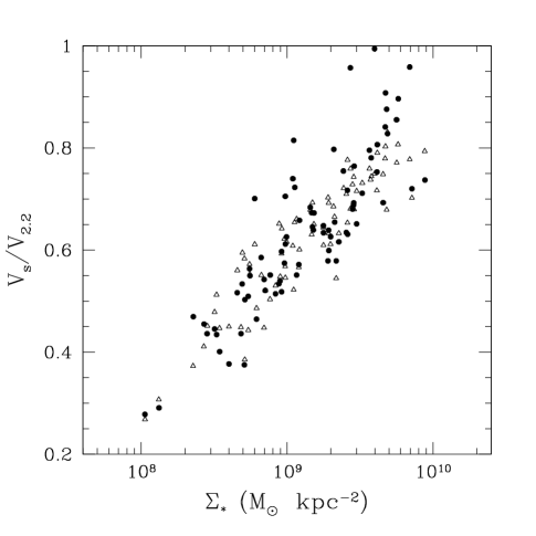
Figure 10.— Contribution of stars to the circular velocity at $2.2R_{d}$ vs. stellar surface density. Filled circles are the data, using the SED-based estimates of the stellar mass, triangles are a realization of our best-fit model with $\bar{m}_{d}\propto\Sigma_{*}^{p_{2}}$, including the AC effect. Left panel: Kroupa IMF, right panel: light IMF.

One of the persistent issues in disk galaxy studies is the role of disk gravity in determining the rotation curve. In “maximal disk” models, the disk typically contributes $75\%-95\%$ of the rotational support at $2.2R_{d}$ (Sackett, 1997). Solid points in the left panel of Figure 10 show the ratio of the circular velocity from the stellar disk to the measured circular velocity $V_{2.2}$ for our observed sample, assuming a Kroupa IMF (similar to Fig. 7 of Pizagno et al. 2005). The contribution of stars to the circular velocity at $2.2R_{d}$ increases monotonically with the stellar surface density. Most of the galaxies with $\Sigma_{*}>3\times 10^{9}\,\mathrm{M}_{\odot}\,{\rm kpc}^{-2}$ are maximal disk by Sackett’s criterion, while the less dense disks are dark matter-dominated. Open points show the same ratio for the model realization shown in the lower panel of Figure 8, with $\bar{m}_{d}\propto\Sigma_{*}^{0.65}$ and AC. The model shows the same trend as the data, except that there are essentially no model galaxies with $V_{s}/V_{2.2}>0.8$. Ratios higher than this imply such small halos (relative to the galaxy baryon mass) that our model never predicts them. The right panel of Figure 10 shows the same results for the light IMF. Note that the observational data points also change in this case, because the value of $M_{*}$ inferred for each galaxy is lower and the values of $\Sigma_{*}$ and $V_{s}$ are therefore lower as well. Only two observed galaxies have $V_{s}/V_{2.2}>0.8$ in this case, while the rest have sub-maximal disks. The correlation of the ratio $V_{s}/V_{2.2}$ with $\Sigma_{*}$ is stronger than with $M_{*}$ or other available galaxy parameters. This reinforces the assumption of our models that the surface density is a major factor regulating the stellar mass fraction of disk galaxies.

Figure 11 shows the distributions of the disk angular momentum parameter for the two models of Figure 8. These $\lambda_{d}$ histograms are qualitatively similar to those for the constant–$m_{d}$ models shown in Figure 5. The typical $\lambda_{d}$ values again increase with the typical values of $m_{d}$. The mode values are $\bar{\lambda}_{d}\approx 0.054$ for the AC model and $\bar{\lambda}_{d}\approx 0.036$ for the no–AC model, compared to $\bar{\lambda}\approx 0.045$ for dark matter halos. For visual clarity, we have omitted the light–IMF model from Figure 11, but its $\lambda_{d}$ histogram is intermediate between the other two, with $\bar{\lambda}_{d}\approx 0.040$. All three model distributions are narrower than the corresponding $P(\lambda)$ for dark matter halos: $\sigma_{\lambda d}\approx 0.25$ (AC), 0.39 (no AC), 0.34 (light IMF) vs. $\sigma_{\lambda}\approx 0.56$. Furthermore, our procedure should overestimate the true width of the $\lambda_{d}$ histogram because we choose a random value of $m_{d}$ from $P(m_{d}|M_{*},R_{d})$, thus adding artificial scatter to the $\lambda_{d}$ values given the $R_{d}$ constraints. (We do not expect to draw the correct value of $m_{d}$ on a galaxy-by-galaxy basis, even if our model incorporates the correct spread of $m_{d}$ values.) To test the magnitude of this effect, we have applied our procedure to a realization of the AC model, choosing new, random values of $m_{d}$ and $c$ for each model galaxy. The input $\lambda_{d}$ distribution has a standard deviation $\sigma_{\lambda d}=0.25$, while the distribution inferred by fitting the model data points has $\sigma_{\lambda d}=0.34$, nearly 40% larger. The mean value $\bar{\lambda}_{d}$ is reproduced correctly. Thus the $\lambda_{d}$ distributions shown in Figure 11 place strong constraints on the allowed values of the angular momentum parameter of disk-dominated galaxies. These distributions are quite different from the $\lambda$ distribution of $N$-body halos, implying that only a subset of halos form disk galaxies like those in our sample, or that disk baryons have systematically different angular momenta from the dark matter.

Figure 11.— Distribution of disk angular momentum parameter required by our best-fit models with $\bar{m}_{d}\propto\Sigma_{*}^{p_{2}}$ with AC (solid histogram) and without AC (dashed histogram). Dotted hatched histogram shows the $P(\lambda)$ distribution of dark matter halos as in Fig. 5.

Dutton et al. (2006, hereafter DVDC) have recently carried out an investigation that is similar to ours in many respects, though in spirit theirs is more a theoretical modeling study constrained by data while ours is an empirical inference study informed by theory. The observational results from their large compilation of three $I$-band TF data sets ($\sim$ 1300 galaxies with H$\alpha$ rotation curves) agree well with those from our smaller, homogeneous data set, which is reassuring given the numerous differences in sample selection, observations, analysis methods, and typical galaxy distances (which strongly affect the observational error budget because of peculiar velocities). In particular (see Fig. 3 of DVDC) we find similar TF slope and intercept and similar lack of correlation between TF residual and radius residual; our galaxies have slightly larger average scale lengths at fixed luminosity, which is plausibly an effect of our stricter limit on bulge-to-disk ratio. DVDC’s estimated intrinsic scatter of 0.052 dex in $\log V_{2.2}$ at fixed $I$-band luminosity, inferred by subtracting observational errors in quadrature from the total scatter, is only marginally larger than our maximum-likelihood estimate of the intrinsic scatter at fixed stellar mass, $\sigma=0.049\pm 0.007$ dex. This similarity is somewhat surprising, since the scatter at fixed luminosity should be increased by galaxy-to-galaxy scatter in $I$-band mass-to-light ratios. Furthermore, if DVDC included distance uncertainties in their observational error budget, their estimate of the intrinsic scatter would decrease, coming closer to our value or perhaps even falling below it.

There are many differences of detail in our theoretical modeling methods: we model relations involving estimated stellar masses while DVDC use $I$-band luminosities; we infer $\lambda_{d}$ distributions by fitting individual $R_{d}$ values while DVDC assume a log-normal $\lambda_{d}$ distribution of adjustable width; and we adopt a Kroupa (2001) IMF as our standard while DVDC take Bell & de Jong’s (2001) “diet Salpeter” IMF as fiducial. Despite these differences, our qualitative theoretical conclusions are largely concordant to the extent that they can be compared. Both studies infer a narrow distribution of $\lambda_{d}$ relative to N-body predictions for the halo $\lambda$ distribution. DVDC do not consider models with $m_{d}$ connected to $\Sigma_{*}$. However, their surface density threshold for star formation has an effect of the same sign (since they define $m_{d}$ in terms of baryonic mass while we define it in terms of stellar mass), and they find that this threshold plays an important role in suppressing TF residual correlations. We find that scatter in $m_{d}$ is required to reproduce the observed TF scatter, while DVDC do not. Given the similar observational estimates of the intrinsic scatter, this difference probably arises largely because DVDC incorporate scatter in $I$-band stellar mass-to-light ratios while we use $g-r$ color to estimate $M/L_{i}$ and assume no scatter about the mean relation. DVDC emphasize the galaxy luminosity function as an additional constraint on models, and we will take up this point ourselves in §4 below (see Figure 14). We concur with DVDC that omitting adiabatic contraction, adopting a lighter IMF, or lowering halo concentrations (see §4) all help to improve agreement with the observed TF relation (including residual correlations) and to reduce the tension between the TF relation and the galaxy stellar mass function (or luminosity function). We are more skeptical about the physical plausibility of omitting (or, in DVDC’s favored model, reversing) the effects of adiabatic contraction, for the reasons cited in §1, so we lean towards some combination of light IMF and lower halo concentration as a more likely explanation.

3.3. Individual galaxy (“exact”) fit models

A common approach in modeling the TF relation has been to choose a distribution $P(\lambda_{d})$ a priori (Kauffmann et al., 1993; Dalcanton et al., 1997; Mo et al., 1998; van den Bosch, 2000). In the previous sections, we have modified this approach by choosing $\lambda_{d}$ to match the observed disk scale length $R_{d}$ on a galaxy-by-galaxy basis. In doing so, we have derived an empirical estimate of $P(\lambda_{d})$, given the model distribution $P(m_{d}|M_{*},R_{d})$. We can go one step further and choose $m_{d}$ for each galaxy to exactly reproduce its observed velocity $V_{2.2}$. We still assume that the dark matter halos are described by the NFW model with a concentration parameter dependent on $M$. Models constructed in this way reproduce the observed $M_{*}$, $R_{d}$, and $V_{2.2}$ distributions by construction, and they yield $P(m_{d})$ as a result.

Jimenez et al. (2003) follow this approach to estimate the disk mass fractions and angular momentum parameters from a large sample of H$\alpha$ rotation curves, assembled from various sources. They consider cuspy NFW models and cored pseudo-isothermal spheres for the dark halos and apply the standard model of adiabatic contraction (e.g., Blumenthal et al., 1986). In contrast to our procedure, they do not use stellar mass-to-light ratios estimated from galaxy colors but instead treat $M_{*}/L$ as an additional fitting parameter for each galaxy.

There are two reasons why we do not adopt this “exact fit” method as our main approach. First, we choose the concentration parameter at random from the distribution $P(c)$, and since the inferred disk mass fraction is sensitive to the value of $c$, the $m_{d}$ values are not accurate on a galaxy-by-galaxy basis. Second, observational errors on $M_{*}$, $R_{d}$, and $V_{2.2}$ introduce substantial uncertainty in the derived values of $m_{d}$, even if the assumed concentration is correct. (The same effect influences the $\lambda_{d}$ values in our standard approach, but much more weakly.) Despite these shortcomings, it is interesting to compare the $P(m_{d})$ estimated by this “exact fit” approach to the distribution assumed in the best-fit models of section 3.2.

Figure 12.— Disk mass fractions that reproduce the observed rotation velocities exactly for models with AC and two stellar IMFs: Kroupa IMF (left panel), light IMF (right panel). Vertical error bars illustrate the uncertainty associated with the scatter of halo concentrations. The end points correspond to $\log{c}\pm\sigma_{c}$, with $\sigma_{c}=0.14$. The value of $m_{d}$ is not allowed to exceed 0.5. Lines show the mean trend (solid) and $1\,\sigma$ scatter (dashed) of the best-fit models with AC (eq. [13]) for each IMF.

Figure 12 plots the inferred values of $m_{d}$ against $\Sigma_{*}$, assuming AC and a Kroupa IMF (left panel) or a light IMF (right panel). Points show the $m_{d}$ value determined for a halo concentration $c=\bar{c}(M)$. Error bars show the effect of raising or lowering the log of the concentration by $\pm\sigma_{c}$ (0.14 dex). For higher $c$, the total halo mass must be lower to produce the same $V_{2.2}$, and the value of $m_{d}=M_{*}/M$ is consequently higher. We have also tried varying the values of $M_{*}$, $R_{d}$, and $V_{2.2}$ by their $1\,\sigma$ observational errors, and these variations on their own produce an $m_{d}$ spread similar to that shown by the error bars in Figure 12.

Lines in the left panel of Figure 12 show the mean trend and $1\,\sigma$ scatter of our best-fit Kroupa–IMF model from §3.2. The trend of the “exact fit” points is qualitatively similar to that of the model. However, there are a number of galaxies that cannot be fit with an $m_{d}$ value below the universal baryon fraction of 0.17, for any value of $c$ in the expected range. (We have arbitrarily imposed an upper limit of 0.5 on $m_{d}$ in Figure 12.) These are the “maximal disk” galaxies from Figure 10, which cannot be fit by an adiabatically contracted NFW halo with typical concentration. If we omit adiabatic contraction, some but not all of these points move to $m_{d}<0.17$. For the light IMF, only four galaxies require $m_{d}>0.17$ for a concentration in the expected range. The smaller number of physically peculiar results in this case is a circumstantial argument in favor of the light IMF.

It is tempting to go further and examine, for example, the correlation between $m_{d}$ and $\lambda_{d}$ (see Jimenez et al., 2003). Unfortunately, we consider correlations derived in this way to be unreliable. Adopting an incorrect value of $c$ for an individual galaxy leads to an incorrect $m_{d}$, and the inferred value of $\lambda_{d}$ for that galaxy adjusts in a correlated way to reproduce the observed disk scale length $R_{d}$. If we take an input model that has no correlation between $m_{d}$ and $\lambda_{d}$, we find that this effect produces a strong, spurious correlation between the “exact fit” values of $m_{d}$ and $\lambda_{d}$. A similar spurious correlation arises from observational errors, as we illustrate in Figure 13. For this test, we create an artificial input sample by choosing the constant values of $\lambda_{d}=0.05$ and $m_{d}=0.08$ for all observed galaxies and recalculating $R_{d}$ and $V_{2.2}$ accordingly, while keeping the observed $M_{*}$ and the mean halo concentration $\bar{c}(M)$. Then we generate a realization of the new sample with added random “measurement” errors of $M_{*}$, $R_{d}$, $V_{2.2}$ and perform the “exact fit”, assuming a halo concentration drawn from $P(c)$. The inferred values of $m_{d}$ and $\lambda_{d}$ scatter along the lines of $\lambda_{d}\propto m_{d}^{1/2}$ at high $m_{d}$ and $\lambda_{d}\propto m_{d}^{2/3}$ at low $m_{d}$, displaying a spurious correlation. It might be possible to investigate the correlation of $m_{d}$ and $\lambda_{d}$ by fitting resolved rotation curves and thus deriving the halo concentration for each galaxy, but even in this case one should be cautious of the impact of observational errors.

We have also investigated the dependence of inferred values of $m_{d}$ and $\lambda_{d}$ on $\Sigma_{*}$. The underlying question is: Do low surface brightness galaxies have low density because of low $m_{d}$ (feedback or inefficient star formation) or because of high $\lambda_{d}$ (high angular momentum)? We use the radius residual, $\Delta R_{d}$, relative to the mean $R_{d}-M_{*}$ relation as our measure of surface density variation at fixed $M_{*}$. For our best-fit AC, Kroupa–IMF model we find only a weak anti-correlation between $\Delta R_{d}$ and $m_{d}$, but we do find a significant positive correlation between $\Delta R_{d}$ and $\lambda_{d}$ (correlation coefficient is 0.63). Thus in our best-fit model, the low-density galaxies tend to have both lower $m_{d}$ (a feature built into the model by the $m_{d}-\Sigma_{*}$ correlation) and higher $\lambda_{d}$, but the $\lambda_{d}$ variations dominate the spread of surface density at fixed $M_{*}$. We are unable to confirm or reject this trend using our “exact fit” procedure, because any correlation is washed out by observational uncertainties and by scatter of halo concentrations. Figure 13 shows that the inferred values of $m_{d}$ and $\lambda_{d}$ are scattered similarly for the high and low surface density galaxies. Even when we create another artificial input sample with an encoded anti-correlation of $\lambda_{d}$ and $\Sigma_{*}$, the recovered values of $\lambda_{d}$ are completely uncorrelated with $\Sigma_{*}$.

Figure 13.— Scatter in the inferred “exact-fit” values of $m_{d}$ and $\lambda_{d}$ resulting from observational errors in $M_{*}$, $R_{d}$, $V_{2.2}$ and from scatter of halo concentrations. The dotted lines show two power-law trends, $\lambda\propto m_{d}^{1/2}$ and $\lambda\propto m_{d}^{2/3}$, respectively. True values were set to $m_{d}=0.08$ and $\lambda_{d}=0.05$ (at the intersection of the dotted lines). Solid squares and open circles correspond to galaxies with $\Sigma_{*}$ above and below $10^{9.2}\,\mathrm{M}_{\odot}\,{\rm kpc}^{-2}$, respectively.

4. Additional constraints

So far, we have constrained the distribution of disk mass fractions using only the TF relation and its residuals, or the FP relation. In this section, we compare the best-fit models from §3.2 to additional observational constraints from the stellar mass function of galaxies and from the extended mass profiles around galaxies probed by weak lensing and satellite dynamics. For brevity, we will refer to the three models shown in Figures 8 and 9, all of which incorporate $\bar{m}_{d}\propto\Sigma_{*}^{p_{2}}$, as the AC, no–AC, and light–IMF models.

Given our best-fit $P(m_{d}|M_{*},R_{d})$, we can go from a cosmological model prediction of the abundance of dark matter halos to a prediction of the number density of disk galaxies as a function of stellar mass. To make such predictions we use the halo mass function calculated by the ellipsoidal excursion set method of Sheth & Tormen (2002), which accurately describes the results of cosmological $N$-body simulations (e.g., Springel & et al., 2005). We adopt cosmological parameters of a $\Lambda$CDM model, $\Omega_{\rm m}=1-\Omega_{\Lambda}=0.24$, $\Omega_{\rm b}=0.041$, $\sigma_{8}=0.74$, $n=1$, $H_{0}=70$ km s^-1 Mpc^-1, favored by the WMAP 3-year data set and a variety of other cosmological observables (Spergel & et al., 2006). Note, however, that our adopted $\bar{c}(M)$ is calibrated on simulations with higher $\sigma_{8}$, a point we will return to shortly. We use the models defined by equation (13) to convert the halo masses $M$ to stellar masses $M_{*}$. First, we use the mean mass-radius relation (eq. [3]) to express the average surface density as a function of stellar mass, $\Sigma_{*}\propto M_{*}^{0.52}$, and convert the density-dependent model $\bar{m}_{d}(\Sigma_{*})$ to the mass-dependent $\bar{m}_{d}(M_{*})$. This procedure yields similar but not identical functions to those given by equation (12). Then we integrate equation (11) to obtain the mean disk mass fraction for galaxies of mass $M_{*}$: $\left<m_{d}\right>(M_{*})\equiv\int m_{d}P(m_{d}|M_{*})d\log{m_{d}}$, with an upper limit $m_{d}=0.15$. Finally, we convert stellar mass to the mean halo mass, $\left<M\right>=M_{*}/\left<m_{d}\right>(M_{*})$, and shift the halo mass function to a galaxy mass function, $dn_{\rm gal}(M_{*})/d\ln{M_{*}}\equiv dn_{\rm halo}({\left<M\right>})/d\ln{M}$.

Our calculation implicitly assumes that each dark matter halo hosts one and only one disk galaxy, so it does not include the contribution of satellite galaxies to the galaxy mass function. However, theoretical models and observational estimates from galaxy clustering and galaxy-galaxy lensing all indicate that the fraction of galaxies that are satellites in the mass range of our sample is low, between 10% and 20% (Mandelbaum et al., 2005; Zehavi & et al., 2005; Zheng et al., 2005).

Figure 14 shows the theoretical halo mass function, the galaxy stellar mass functions predicted by the AC, no–AC, and light–IMF models, and the observational estimate of this mass function by Bell et al. (2003), derived from the SDSS and 2MASS surveys. We have converted this estimate from Bell et al.’s “diet-Salpeter” IMF to a Kroupa IMF by multiplying their galaxy mass parameters by $10^{-0.15}$. The AC model substantially over-predicts the observed mass function at all masses, even without accounting for satellite galaxies. The high values of $m_{d}$ required to match the TF relation with a Kroupa IMF and AC puts galaxies of a given $M_{*}$ into relatively low-mass, abundant halos, leading to a high number density. This tension between the galaxy luminosity function and the Tully-Fisher relation is a long-standing problem for CDM-based models of galaxy formation (e.g., Kauffmann et al., 1993; Cole et al., 1994; Somerville & Primack, 1999). Here we are essentially confirming this problem, but removing some sources of uncertainty by using stellar masses in place of luminosities and by applying TF constraints from a well defined galaxy sample. Of course, some of the halos in this range ($V_{\rm vir}=80-300$ km s^-1) might host galaxies with significant bulges, which would not be in our TF sample – about 50% of the galaxies in Pizagno et al.’s (2006, in preparation) full sample satisfy the bulge-to-total $<0.1$ criterion used here. However, if we lower the predicted mass function to account for the fraction of galaxies with substantial bulges, then we should also lower the observed mass function by the same factor, leaving the same gap between them. Reconciling the AC model with the Bell et al. (2003) estimate for a Kroupa IMF requires, instead, that the halos that do not host disk-dominated galaxies have drastically lower values of $m_{d}$, making them “dim” or “dark”.

Figure 14.— Predicted mass functions of disk galaxies for the best-fit models with $\bar{m}_{d}\propto\Sigma_{*}^{p_{2}}$ with AC (dot-dashed line), without AC (dotted line), with AC and light stellar IMF (dashed line), and with low $\bar{c}(M)$ (long-dashed line). These galaxy number densities are calculated from the abundance of dark matter halos in the concordance $\Lambda$CDM cosmology as a function of galaxy stellar mass, $M_{*}=m_{d}M$, with the model values of $m_{d}(M)$ in each case. For comparison, top solid line (labeled “halos”) shows the case if the halos converted all of their baryons into stars. Bottom solid curve (labeled “galaxies”) shows the observed mass function of galaxies in the local universe from Bell et al. (2003). The plotted range of masses corresponds to the range of rotation velocities $80-300$ km s^-1, covered by our observed sample.

The dotted curve in Figure 14 shows the prediction of the no–AC model, which lies below the Bell et al. (2003) estimate near the knee of the mass function but rises above it at low and high masses. We do not view the discrepancy above $10^{11}\,\mathrm{M}_{\odot}$ as a serious problem, because a large fraction of galaxies in this mass range are early-type systems, which could plausibly have $m_{d}$ values lower by a factor $\sim 2$, and because massive halos have a larger fraction of their baryon mass in satellite galaxies and intergalactic gas, leaving less for the central galaxy. The tension below $M_{*}\sim 2\times 10^{10}\,\mathrm{M}_{\odot}$ is more significant, since our sample extends to $2\times 10^{9}\,\mathrm{M}_{\odot}$ and most galaxies in this mass range are late types, but it is arguably within the systematic uncertainties of the model and the data. We therefore consider the no–AC model to be an empirically acceptable way to reconcile the TF and mass function constraints, albeit one that requires abandoning a seemingly well established element of galaxy formation physics.

The dashed curve in Figure 14 shows the model with adiabatic contraction and a light stellar IMF. Rather than plot a second version of the “observed” mass function, we have added 0.15 dex back to the model values of $M_{*}$, thus allowing a direct comparison to the original observational curve. If changing the IMF simply lowered $m_{d}$ values by 0.15 dex, then the predicted and observed mass functions would shift by the same factor, and the agreement between them would not improve. However, because the light IMF reduces the effect of disk gravity (both the direct contribution and the magnitude of AC), it lowers the ratios $V_{2.2}/V_{\rm vir}$ and reduces average $m_{d}$ values by nearly a factor of two. This reduction improves the agreement with observations by putting galaxies in halos of higher mass and lower abundance. The light–IMF model with AC lies midway between the Kroupa–IMF models with and without AC. It is marginally consistent with the Bell et al. (2003) mass function.

A third way to reconcile the TF and mass function constraints is to change cosmological parameters, and thus the halo mass function. We find that lowering the matter density parameter to $\Omega_{\rm m}\approx 0.15$ brings the prediction of Kroupa–IMF, AC model low enough to match the knee of the observed mass function, and it also brings the light–IMF, AC model into rough alignment with the Kroupa–IMF, no AC model. Changing the power spectrum normalization, $\sigma_{8}$, on the other hand, has little impact on the predicted $n(M_{*})$ because the halo mass function is only weakly sensitive to $\sigma_{8}$ in this mass range.

This discussion of the effects of changing cosmological parameters ignores the potentially crucial impact of $\sigma_{8}$ on halo concentrations. Bullock et al. (2001b) present an analytic model for predicting halo concentrations (see also Kuhlen et al., 2005), calibrated against their $\Omega_{\rm m}=0.3$, $\sigma_{8}=1.0$ $\Lambda$CDM simulation. If we apply this model to the WMAP 3-year cosmological parameters, we obtain concentrations lower by about 25% at fixed mass, mainly because of the lower value of $\sigma_{8}$. In the range $M=10^{11}-10^{13}\,h^{-1}\mathrm{M}_{\odot}$, the analytic model prediction is well fit by a power law, $\bar{c}(M)\approx 9\,(M/10^{12}\,h^{-1}\mathrm{M}_{\odot})^{-0.1}$. We have not adopted this as our standard relation for the calculations above because the $\sigma_{8}$ dependence of halo concentrations has not been thoroughly tested against $N$-body simulations. However, the preliminary tests that have been carried out to date, and the tests of the predicted redshift dependence of concentrations, suggest that the analytic model is accurate (J. Bullock, private communication).

The last lines of Tables 1 and 2 list TF and FP results for a model similar to our best-fit Kroupa–IMF, AC model with $\bar{m}_{d}\propto\Sigma_{*}^{0.65}$, but using this lower $\bar{c}(M)$ relation. Lower concentrations place a smaller fraction of the halo mass within $2.2\,R_{d}$, and therefore the total halo mass must be larger to reproduce the observed $V_{2.2}$. The best-fit value of $\bar{m}_{d,0}$ (defined at $M_{*}\,R_{d}^{-2}=10^{9.2}\,\mathrm{M}_{\odot}\,{\rm kpc}^{-2}$, see eq. [13]) drops from 0.1 to 0.04. For a galaxy with the mean $\bar{c}(M)$ that lies on the mean $R_{d}-M_{*}$ relation, this change of normalization keeps the mass of the adiabatically-contracted NFW halo within $2.2\,R_{d}$ approximately the same as before. Lowering $\bar{c}(M)$ and $\bar{m}_{d,0}$ yields a slightly better fit to the TF relation, with weaker residual anti-correlation but slightly worse slope and intercept, and a noticeably better fit to the FP relation. However, the improvement in the predicted mass function is dramatic, as shown by the long-dashed curve in Figure 14, because the lower $m_{d}$ values put galaxies in more massive, less abundant halos. The low $\bar{c}(M)$, AC model fares just slightly worse than the high $\bar{c}(M)$, no–AC model in the mass function test.

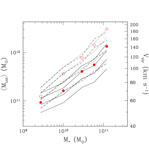
Figure 15.— Average mass enclosed within 50, 100, 200, and 400 kpc (bottom to top) of galaxy centers as a function of stellar mass for the best-fit models with $\bar{m}_{d}\propto\Sigma_{*}^{p_{2}}$, with AC (solid lines), without AC (dotted lines), and with AC and light stellar IMF (dashed lines). Pentagons show the average halo virial mass for the standard IMF, with AC (filled) and without AC (open).

Using our best-fit models, we can also make predictions for extended mass distributions around galaxies like those in our sample. Figure 15 shows the mean total mass enclosed within a fixed distance from the galaxy center, for distances ranging from $d=50$ kpc to $d=400$ kpc. For each galaxy in our sample, we use one realization of each model to calculate the interior mass $M_{\rm int}(<d)$ as a sum of the observed stellar mass and the predicted dark halo mass with the NFW profile. The distribution of gas (if present) is implicitly assumed to follow the distribution of dark matter. At these large distances, we ignore the effect of AC on the shape of the NFW profile, although the model $m_{d}$ values are of course determined taking AC into account at $2.2\,R_{d}$. We average $M_{\rm int}(<d)$ in five bins of stellar mass containing approximately equal number of galaxies, and plot the mean $M_{\rm int}(<d)$ against the average stellar mass $\left<M_{*}\right>$ in the bin. For the AC and no–AC models, we also show the bin average of the virial mass (for critical overdensity $\Delta=101$), with the corresponding virial velocity marked on the right axis. The interior masses for the no–AC model are higher than those of the AC model, typically by factors of $1.5-2$, because of the lower $m_{d}$ values. The dependence of $M_{\rm int}(<d)$ on $M_{*}$ is shallower for the AC model because of the stronger dependence of $\bar{m}_{d}$ on $\Sigma_{*}$, which puts lower mass (and generally lower $\Sigma_{*}$) galaxies in more massive halos. The predicted interior mass in the models with $\bar{m}_{d}\propto M_{*}^{p_{1}}$ is similar to that in the corresponding models with $\bar{m}_{d}\propto\Sigma_{*}^{p_{2}}$. Predictions of the light–IMF model are close to those of the no–AC model, since they have similar values of $m_{d}$. Predictions of the Kroupa–IMF model with AC and low $\bar{c}(M)$ are also similar to those of the plotted no–AC model at $d\leq 100$ kpc, but they lie systematically above it at larger $d$ because the halos are more extended.

These extended mass distributions can probed by galaxy-galaxy weak lensing observations, which yield the mean total mass profiles after stacking a large number of galaxies of similar luminosity or stellar mass. To compare with such measurements, we plot in Figure 16 the virial mass-to-light ratios in $r$-band, $M_{\rm vir}/L_{r}$, predicted by the AC models with the Kroupa IMF and the light IMF. For each galaxy in our sample, we draw $m_{d}$ values and concentrations from the $P(m_{d}|M_{*},R_{d})$ and $P(c)$ distributions 10 times and compute the average $M_{\rm vir}$, then divide by the galaxy’s observed $L_{r}$. We follow the conventional practice of lensing studies in using $L_{r}$ not corrected for internal extinction (which differs from standard practice in TF studies). Pentagonal points with error bars show virial mass-to-light ratios of late-type galaxies estimated by Mandelbaum et al. (2005), based on galaxy-galaxy lensing measurements in the SDSS. These ratios, ranging from $\sim 40-130\,\mathrm{M}_{\odot}/\mathrm{L}_{\odot}$, are consistent with the light–IMF model but too high for the AC, Kroupa–IMF model. Star symbols with error bars show the galaxy-galaxy lensing results of Hoekstra et al. (2005) using the Red-Sequence Cluster Survey, which are somewhat lower and overlap with the predictions of both models. Results for the Kroupa–IMF models with no AC and with AC but low $\bar{c}(M)$, not shown in the Figure, are similar to those of the light–IMF model with AC.

An independent measure of the dynamical mass at large distances from the galaxy center is provided by the dynamics of satellite galaxies. Using a large sample of SDSS galaxies, Prada et al. (2006, in prep.) estimate $M_{\rm vir}=2.4\times 10^{12}\,\mathrm{M}_{\odot}$ for the average luminosity $L_{r}=1.8\times 10^{10}\,\mathrm{L}_{\odot}$ (open triangle in Figure 16). After converting luminosity to stellar mass, this corresponds to $m_{d}=0.028$, below our best-fit values at this $M_{*}$ ($\bar{m}_{d}=0.11$ and 0.044, for the Kroupa–IMF and light–IMF models with AC, respectively, and $\bar{m}_{d}=0.042$ for the no–AC model). Note that this estimated mass fraction applies to an average of galaxies of all types, which could plausibly lie below the mass fraction of disk-dominated galaxies in our sample. Stellar spheroids (bulges and elliptical galaxies) have higher stellar mass-to-light ratios than younger disk systems, so they have higher $M_{\rm vir}/L$ even for the same $M_{*}/M_{\rm vir}$. Mandelbaum et al. (2005) find an average $M_{\rm vir}/L_{r}$ of 140 for early-type galaxies vs. 53 for late types in the luminosity range $L_{r}=10^{10}-10^{11}\,\mathrm{L}_{\odot}$. Furthermore, recent studies suggest that bulge-dominated galaxies have lower values of $M_{*}/M_{\rm vir}$. For example, Humphrey et al. (2006) find a stellar fraction of 0.044 for an X-ray model of an elliptical galaxy NGC 720, while Hoekstra et al. (2005) find on the average 2.5 times lower $M_{*}/M_{\rm vir}$ for the red ($B-V>0.8$) galaxies than the blue galaxies. Galaxies composed of a mixture of the disk and spheroidal components would have lower average $M_{*}/M_{\rm vir}$ than pure disk-dominated galaxies, and this difference may contribute to the gap between our AC models and the Prada et al. (2006) measurement.

Available cosmological gasdynamics simulations of disk-dominated galaxies, which automatically include the halo response to baryon condensation, predict $m_{d}$ values in the same general range as our models. In a realization of 19 Milky Way-type galaxies, Sommer-Larsen (2006) finds a mean baryon mass fraction $m_{d}=0.08$ at $V_{c}=200$ km s^-1. The TF relation for this simulated sample is roughly consistent with our observed relation (Portinari & Sommer-Larsen, 2006), though the sample is too small to investigate residual correlations. For a single galaxy studied with ultra-high resolution, Robertson et al. (2004) also find $m_{d}\approx 0.08$, while for a sample of three disk galaxies Governato et al. (2006) find values of $m_{d}$ between 0.04 and 0.08.

Figure 16.— Dynamical mass-to-light ratio in the $r$-band, $M_{\rm vir}/L_{r}$, for the best-fit AC models with $\bar{m}_{d}\propto\Sigma_{*}^{p_{2}}$, for Kroupa IMF (filled squares and circles) and light IMF (open squares and circles). In both cases, squares correspond to compact galaxies with $R_{d}<\bar{R}_{d}(M_{*})$ (eq. [3]), while circles correspond to extended galaxies with $R_{d}\geq\bar{R}_{d}(M_{*})$. Plotted luminosities $L_{r}$ are the observed values, not corrected for internal extinction. Star symbols with error bars show the galaxy-galaxy weak lensing measurements from Hoekstra et al. (2005), while open pentagons are from Mandelbaum et al. (2005). Open triangle shows an average measurement using satellite dynamics from Prada et al. (2006, in prep.).

All of our best-fit models introduce a correlation of $\bar{m}_{d}$ with $\Sigma_{*}$, which counteracts the tendency of disk gravity to produce higher rotation speeds in more compact galaxies. For the model points in Figure 16, circles and squares respectively shows results for galaxies above and below the mean $R_{d}$ at a given $M_{*}$ (eq. [3]). Larger $R_{d}$ galaxies have systematically higher $M_{\rm vir}/L_{r}$ because they reside in more massive halos. If we divide the sample into three equal-size subsamples containing the smallest, intermediate, and largest galaxies for their $M_{*}$, the mean Kroupa–IMF $M_{\rm vir}/L_{r}$ values are 20, 23, and 28, respectively, and light–IMF $M_{\rm vir}/L_{r}$ values are 42, 46, and 60, respectively. Galaxy-galaxy lensing analyses could test our proposed explanation of the weak correlation between TF residuals and radius, by detecting or ruling out this difference, roughly 40% between the smallest and largest 1/3 of the population.

Measurements of the rotation speed at distances larger than $2.2\,R_{d}$ may also help to differentiate among our proposed best-fit models. High density galaxies in our models have relatively smaller dark matter halos and, therefore, more steeply falling rotation curves at large distances than low density galaxies. As an example, we consider hypothetical measurements, $V_{3.2}$, of the rotation velocity at $3.2\,R_{d}$. For the AC, Kroupa–IMF model, the average ratio $V_{3.2}/V_{2.2}$ drops from 1.00 for the lowest-density galaxies in our sample ($M_{*}\,R_{d}^{-2}\approx 2\times 10^{8}\,\mathrm{M}_{\odot}\,{\rm kpc}^{-2}$) to 0.97 for the highest-density galaxies ($M_{*}\,R_{d}^{-2}\approx 7\times 10^{9}\,\mathrm{M}_{\odot}\,{\rm kpc}^{-2}$). For the light–IMF and low $\bar{c}(M)$ models, $V_{3.2}/V_{2.2}$ varies from 1.02 to 0.99 in the same density range. In contrast, for the no–AC model the ratio $V_{3.2}/V_{2.2}$ is always in the range $1.00-1.03$, indicating that the rotation curve is still rising at $3.2\,R_{d}$. Measurements at $4\,R_{d}$ would show a larger difference. In the no–AC model, the ratio $V_{4}/V_{2.2}$ is still close to unity, while in the AC, Kroupa–IMF model it drops from 0.99 to 0.93, for the density range of our sample. This variation corresponds to up to 15 km s^-1 difference in the rotation speed, which could be detectable in a sample of extended, high-precision rotation curves.

5. Conclusions

We have constrained the structural properties of dark matter halos of disk-dominated galaxies using a well-defined sample of 81 late-type galaxies with H$\alpha$ rotation curves, selected from the SDSS redshift survey (Pizagno et al., 2005). We model the Tully-Fisher and fundamental plane relations constructed from the galaxy stellar mass, $M_{*}$, disk scale length, $R_{d}$, and optical H$\alpha$ rotation velocity at $2.2\,R_{d}$, $V_{2.2}$. The stellar mass is determined from the $i$-band luminosity and a stellar mass-to-light ratio estimated from the galaxy’s $g-r$ color. The normalization of these stellar masses depends on the IMF, for which we generally adopt the form of Kroupa (2001). The maximum likelihood fit to the TF relation for our sample is $\log{V_{2.2}}=0.29(\log{M_{*}}-10.5)+2.23$. The FP relation is $\log{V_{2.2}}=0.27(\log{M_{*}}-10.5)+0.085(\log{R_{d}}-0.65)+2.23$. Residuals from the TF relation are weakly, and positively, correlated with residuals from the $R_{d}-M_{*}$ relation. The weakness of this correlation, and the small $R_{d}$ coefficient in the FP relation, imply that the TF relation is a nearly edge-on view of the fundamental plane of disk galaxies.

We define models of the disk galaxy population by the probability distribution function $P(m_{d}|M_{*},R_{d})$ of the disk stellar mass fraction $m_{d}=M_{*}/M_{\rm vir}$, where $M_{\rm vir}$ is the virial mass of the host dark matter halo, assumed to have an NFW profile with the concentration predicted by $N$-body studies. For each sample galaxy, we draw $m_{d}$ from the model distribution, then find the disk angular momentum parameter $\lambda_{d}$ required to reproduce the galaxy’s observed disk scale length. Our standard calculations include the impact of adiabatic contraction (AC) on the halo profile (e.g., Blumenthal et al., 1986; Gnedin et al., 2004), but we also consider models without AC.

Models with a constant value of $m_{d}$ require $m_{d}\approx 0.08$ with AC ($m_{d}\approx 0.04$ without AC) to reproduce the TF intercept and slope. These models under-predict the scatter in the TF relation, even when we include the full range of concentration scatter found in $N$-body simulations of dark matter halos. More importantly, they predict a strong anti-correlation of TF and $R_{d}-M_{*}$ residuals, with more compact galaxies rotating faster at fixed $M_{*}$. Equivalently, they predict an $R_{d}$ coefficient in the FP relation that has the wrong sign and is incompatible with the observed value. Adding random scatter to $V_{2.2}$ values to match the observed intrinsic scatter does not resolve this conflict with the observed residual correlations. The conflicts are more severe for the models with AC because of the stronger impact of disk gravity. The AC models also predict a TF slope that is slightly too steep.

We conclude that a scatter of $m_{d}$ values, with dispersion in $\ln{m_{d}}$ of $\sigma_{m}\approx 0.25$, is required to reproduce the observed scatter of the TF relation, and that models with AC require higher disk mass fractions in higher mass galaxies to reproduce the observed slope. These findings confirm the more qualitative arguments of Pizagno et al. (2005) based on the same data set. We can obtain consistency with the weak TF residual correlation and the small $R_{d}$ FP coefficient by tying the mean disk mass fraction to the stellar surface density. The best-fit model with AC has $\bar{m}_{d}\propto\Sigma_{*}^{0.65}$ and a mean fraction $\bar{m}_{d}=0.1$ at $M_{*}\,R_{d}^{-2}=10^{9.2}\,\mathrm{M}_{\odot}\,{\rm kpc}^{-2}$. Without AC, the best-fit model has a shallower slope, 0.2 instead of 0.65, and a lower normalization, $\bar{m}_{d}=0.04$ at $10^{9.2}\,\mathrm{M}_{\odot}\,{\rm kpc}^{-2}$. The $\bar{m}_{d}-\Sigma_{*}$ correlation counteracts the effect of stronger disk gravity in more compact galaxies. It produces a major improvement for the AC model, and a modest improvement for the no–AC model.

The derived $\lambda_{d}$ distributions for these two models are significantly narrower than the $\lambda$ distribution for dark matter halos in $N$-body simulations: $\sigma_{\lambda d}\approx 0.25$ (AC) or 0.39 (no AC) vs. $\sigma_{\lambda}\approx 0.56$. The mean $\bar{\lambda}_{d}$ depends on the typical $m_{d}$ values, which determine halo virial radii: we find $\bar{\lambda}_{d}\approx 0.054$ (AC) or $\bar{\lambda}_{d}\approx 0.036$ (no AC) vs. $\bar{\lambda}\approx 0.045$ for $N$-body halos. The systematic difference between the $\lambda_{d}$ and $\lambda$ distributions implies either that disk baryons have systematically different angular momentum from the dark matter in their host halo or that only a subset of halos form disk-dominated galaxies like those in our sample.

We consider the $\bar{m}_{d}-\Sigma_{*}$ correlation a physically plausible mechanism for bringing theoretically motivated disk formation models, which include adiabatic contraction, into agreement with the slope and residual correlation of the observed TF relation. However, our best-fit AC model suffers the long-standing problem of over-producing the galaxy stellar mass function given the halo population of a $\Lambda$CDM cosmological model with observationally favored parameter values and the concentration-mass relation of Bullock et al. (2001b). It also predicts virial mass to $r$-band light ratios lower than some recent estimates from galaxy-galaxy lensing and satellite dynamics. Lowering $\Omega_{\rm m}$, and thus the halo mass function, can ameliorate the abundance problem, but the required value, $\Omega_{\rm m}\approx 0.15$, seems implausibly low and the mass-to-light ratio problem remains in any case. Eliminating AC can resolve both problems, at the expense of dropping a well-tested ingredient of galaxy formation theory.

We suggest an alternative solution: adopting a “light” stellar IMF with $M_{*}/L$ lower than the Kroupa (2001) IMF by about 0.15 dex. This model yields acceptable residual correlations with a modest trend $\bar{m}_{d}\propto\Sigma_{*}^{0.4}$, predicts virial mass-to-light ratios in accord with recent measurements, and reduces but does not entirely remove the tension with the galaxy baryon mass function. We do not know of other observational evidence to support such a light IMF, but it is perhaps within the uncertainties of existing observational constraints. Systematic uncertainties in the Bell et al. (2003) population synthesis models, which we use to compute $M_{*}/L$ from $g-r$ color, could account for some of the required change even without altering the IMF itself. We also show that the lower $\bar{c}(M)$ relation predicted for $\sigma_{8}=0.74$ by Bullock et al.’s (2001b) analytic model relieves most of the tension between the TF relation and the mass function and $M_{\rm vir}/L_{r}$ constraints, even in the case of a Kroupa IMF. A full assessment of this solution awaits better numerical confirmation of the analytic model and better observational constraints on $\sigma_{8}$. Other changes to halo profiles that reduce the fraction of mass at small radii would have similar effects.

Our observational findings are consistent with those of Dutton et al. (2006), which is reassuring given the different characteristics of the data sets. Our theoretical inferences are consistent but not identical. We are more reluctant than Dutton et al. (2006) to abandon adiabatic contraction, given the numerous simulations in which it occurs and the absence of any simulations in which it does not. The $\bar{m}_{d}-\Sigma_{*}$ correlation can remove the $\Delta R_{d}-\Delta V_{2.2}$ anti-correlation that otherwise plagues models with AC, though it leaves problems with the baryon mass function and weak lensing mass-to-light ratios. The addition of a light IMF or the adoption of lower halo concentrations largely resolve these difficulties as well, and we consider some combination of these effects to be a plausible resolution of the observational tensions. Modeling of rotation curve data at larger and smaller separations and galaxy-galaxy lensing measurements for more finely divided galaxy sub-classes may provide further insight that could help discriminate among these solutions. The fact that disk formation models based on the most straightforward theoretical and observational inputs do not reproduce all aspects of the current data suggests that interesting surprises may still lie ahead.

Appendix A Multidimensional Linear Fit using Maximum Likelihood

We have developed the following procedure for a multidimensional linear fit to data with observational errors in all variables, allowing for intrinsic Gaussian scatter. Each data point (galaxy) is represented by $n+1$ parameters, $n$-vector $x$ and scalar $y$, and their associated measurement errors, ${\mbox{\boldmath$\sigma$}}_{x}$ and $\sigma_{y}$. We label each galaxy by subscript $i$ and fit a linear relation of the form

$$y={\mbox{\boldmath$a$}}({\mbox{\boldmath$x$}}-{\mbox{\boldmath$x$}}_{0})+b+N(0,\sigma),$$ (A1)

where $a$ is also an $n$-dimensional vector and ${\mbox{\boldmath$x$}}_{0}$ is an arbitrary offset. The term $N(0,\sigma)$ accounts for normally-distributed scatter that is intrinsic to the studied relation and is not accounted for by measurement errors. In the case of the TF relation, such scatter could be due to the variations of the mass-to-light ratio among the galaxies, scatter in the properties of their dark matter halos, etc. We define the likelihood function

$$2\ln{\cal L}=-\sum_{i}\ln{(\sigma^{2}+\sigma_{y,i}^{2}+{\mbox{\boldmath$a$}}^{2}{\mbox{\boldmath$\sigma$}}_{x,i}^{2})}-\sum_{i}{[{\mbox{\boldmath$a$}}({\mbox{\boldmath$x$}}_{i}-{\mbox{\boldmath$x$}}_{0})+b-y_{i}]^{2}\over\sigma^{2}+\sigma_{y,i}^{2}+{\mbox{\boldmath$a$}}^{2}{\mbox{\boldmath$\sigma$}}_{x,i}^{2}}+\,{\rm const}$$ (A2)

and find its maximum using Powell’s direction set method (Press et al., 1992). The direction search is done as a function of $n+1$ variables ($a$ and $\sigma$), since the value of the intercept $b$ can then be calculated analytically:

$$b={\sum_{i}w_{i}[y_{i}-{\mbox{\boldmath$a$}}({\mbox{\boldmath$x$}}_{i}-{\mbox{\boldmath$x$}}_{0})]\over\sum_{i}w_{i}},\qquad w_{i}\equiv{1\over\sigma^{2}+\sigma_{y,i}^{2}+{\mbox{\boldmath$a$}}^{2}{\mbox{\boldmath$\sigma$}}_{x,i}^{2}}.$$ (A3)

We estimate the errors of the best-fit parameters ($\Delta$$a$, $\Delta b$, $\Delta\sigma$) by bootstrapping the data. The error estimates are taken to be the standard deviation of the corresponding distributions of the best-fit parameters. We found empirically that of the order 1000 bootstrap realizations are needed in order to obtain robust estimates of the errors, accurate to 3%.

The offset ${\mbox{\boldmath$x$}}_{0}$ can be chosen so as to minimize the uncertainty $\Delta b$ and eliminate correlation between $\Delta$$a$ and $\Delta b$. The slope of the linear fit ($a$) and its error ($\Delta$$a$) do not depend on the choice of ${\mbox{\boldmath$x$}}_{0}$ because its variation can be absorbed in the value of the intercept $b$. The intrinsic scatter and its error are also unaffected by the choice of ${\mbox{\boldmath$x$}}_{0}$. The error of the intercept $b$, however, does depend on ${\mbox{\boldmath$x$}}_{0}$ and can be minimized by the appropriate choice of the offset. We use Brent’s parabolic interpolation method (if $n=1$) or downhill simplex method (if $n>1$) to find the minimum of $\Delta b$.

Computer code that calculates the best-fit parameters and their error estimates is available from the authors upon request. An independent derivation of this maximum likelihood method and further discussion can be found in D’Agostini (2005).

Table 1Tully-Fisher fit parameters

$\bar{m}_{d}$	$p_{i}$	$\sigma_{m}$	$\sigma_{c}$	AC	$a$	$b$	$\sigma$	$r$	$\chi^{2}$
data					$0.291\pm 0.013$	$2.231\pm 0.006$	$0.049\pm 0.007$	$0.23\pm 0.14$
0.02		0	0	N	0.280	2.265	0.009	$-0.02$	67
0.02		0	0	Y	0.292	2.306	0.014	$-0.20$	171
0.04		0	0	N	0.295	2.232	0.016	$-0.26$	36
0.04		0	0	Y	0.307	2.275	0.023	$-0.41$	84
0.08		0	0	N	0.311	2.196	0.027	$-0.48$	68
0.08		0	0	Y	0.322	2.240	0.034	$-0.57$	46
0.04		0	0.14	N	0.297	2.232	0.041	$-0.22$	13
0.04		0	0.14	Y	0.308	2.276	0.039	$-0.36$	70
0.08		0	0.14	N	0.313	2.196	0.040	$-0.43$	55
0.08		0	0.14	Y	0.323	2.240	0.041	$-0.53$	40
0.04	+$\sigma$	0	0.14	N	0.303	2.233	0.049	$-0.27$	14
0.04	+$\sigma$	0	0.14	Y	0.314	2.276	0.049	$-0.42$	72
0.08	+$\sigma$	0	0.14	N	0.319	2.196	0.049	$-0.51$	60
0.08	+$\sigma$	0	0.14	Y	0.329	2.240	0.049	$-0.65$	52
0.04		0.22	0.14	N	0.298	2.233	0.049	$-0.20$	10
0.08		0.27	0.14	Y	0.320	2.249	0.049	$-0.43$	35
$\bar{m}_{d}\propto M_{*}^{p_{1}}$
0.04	0.1	0.25	0.14	N	0.283	2.234	0.051	$-0.17$	8.7
0.1	0.3	0.21	0.14	Y	0.291	2.239	0.046	$-0.45$	25
$\bar{m}_{d}\propto\Sigma_{*}^{p_{2}}$
0.04	0.2	0.25	0.14	N	0.282	2.234	0.051	$-0.07$	5.4
0.1	0.65	0.2	0.14	Y	0.281	2.243	0.041	$-0.18$	14
0.04	0.4	0.24	0.14	N	0.266	2.236	0.051	$+0.02$	6.9
0.1	0.9	0.2	0.14	Y	0.264	2.247	0.044	$-0.08$	16
$\bar{m}_{d}\propto\Sigma_{*}^{p_{2}}$, light IMF
0.04	0.4	0.25	0.14	Y	0.273	2.275	0.051	$+0.01$	4.6
$\bar{m}_{d}\propto\Sigma_{*}^{p_{2}}$, low $\bar{c}(M)$
0.04	0.65	0.2	0.14	Y	0.279	2.246	0.041	$-0.06$	12

Note – The intercept $b$ is for the offset $\log{M_{*0}}=10.5$. Lines with “+$\sigma$” correspond to models with added measurement errors to match the observed scatter. In the ninth column, $r$ is Pearson’s linear correlation coefficient. We estimate its error by bootstrapping the observed sample. We find that $\Delta r$ depends mainly on the number of objects in the sample, $N$, and approximately equals $N^{-1/2}$. For the light IMF, the observed intercept $b=2.231+0.15\times 0.291=2.275$.

Table 2Fundamental plane fit parameters

$\bar{m}_{d}$	$p_{i}$	$\sigma_{m}$	$\sigma_{c}$	AC	$a_{1}$	$a_{2}$	$b$	$\sigma$	$\chi^{2}$
data					$0.271\pm 0.017$	$0.085\pm 0.054$	$2.233\pm 0.006$	$0.048\pm 0.006$
0.02		0	0	N	0.280	$-0.002$	2.265	0.009	69
0.02		0	0	Y	0.305	$-0.054$	2.305	0.008	184
0.04		0	0	N	0.312	$-0.075$	2.230	0.008	55
0.04		0	0	Y	0.336	$-0.125$	2.272	0.007	111
0.08		0	0	N	0.347	$-0.154$	2.192	0.008	125
0.08		0	0	Y	0.369	$-0.200$	2.234	0.007	104
0.04		0	0.14	N	0.315	$-0.076$	2.230	0.038	18
0.04		0	0.14	Y	0.338	$-0.125$	2.272	0.032	77
0.08		0	0.14	N	0.349	$-0.155$	2.192	0.030	93
0.08		0	0.14	Y	0.370	$-0.201$	2.235	0.024	76
0.04	+$\sigma$	0	0.14	N	0.325	$-0.093$	2.231	0.048	21
0.04	+$\sigma$	0	0.14	Y	0.349	$-0.143$	2.273	0.045	80
0.08	+$\sigma$	0	0.14	N	0.361	$-0.174$	2.192	0.043	96
0.08	+$\sigma$	0	0.14	Y	0.382	$-0.220$	2.235	0.038	76
0.04		0.22	0.14	N	0.315	$-0.075$	2.230	0.047	16
0.08		0.27	0.14	Y	0.361	$-0.172$	2.244	0.038	56
$\bar{m}_{d}\propto M_{*}^{p_{1}}$
0.04	0.1	0.25	0.14	N	0.298	$-0.064$	2.234	0.051	10
0.1	0.3	0.21	0.14	Y	0.332	$-0.177$	2.235	0.035	41
$\bar{m}_{d}\propto\Sigma_{*}^{p_{2}}$
0.04	0.2	0.25	0.14	N	0.287	$-0.018$	2.234	0.051	4.6
0.1	0.65	0.2	0.14	Y	0.296	$-0.066$	2.241	0.039	14
0.04	0.4	0.24	0.14	N	0.261	$+0.022$	2.237	0.051	2.2
0.1	0.9	0.2	0.14	Y	0.270	$-0.022$	2.247	0.043	9.6
$\bar{m}_{d}\propto\Sigma_{*}^{p_{2}}$, light IMF
0.04	0.4	0.25	0.14	Y	0.268	$+0.018$	2.275	0.051	1.8
$\bar{m}_{d}\propto\Sigma_{*}^{p_{2}}$, low $\bar{c}(M)$
0.04	0.65	0.2	0.14	Y	0.283	$-0.017$	2.246	0.041	9.8

Note – The intercept $b$ is for the offsets $\log{M_{*0}}=10.5$ and $\log{R_{d0}}=0.65$. For the light IMF, the observed intercept $b=2.275$.

References

- Barnes & Efstathiou (1987) Barnes, J. & Efstathiou, G. 1987, ApJ, 319, 575
- Barnes & White (1984) Barnes, J. & White, S. D. M. 1984, MNRAS, 211, 753
- Bell et al. (2003) Bell, E. F., McIntosh, D. H., Katz, N., & Weinberg, M. D. 2003, ApJS, 149, 289
- Blumenthal et al. (1986) Blumenthal, G. R., Faber, S. M., Flores, R., & Primack, J. R. 1986, ApJ, 301, 27
- Bryan & Norman (1998) Bryan, G. L. & Norman, M. L. 1998, ApJ, 495, 80
- Bullock et al. (2001a) Bullock, J. S., Dekel, A., Kolatt, T. S., Kravtsov, A. V., Klypin, A. A., Porciani, C., & Primack, J. R. 2001a, ApJ, 555, 240
- Bullock et al. (2001b) Bullock, J. S., Kolatt, T. S., Sigad, Y., Somerville, R. S., Kravtsov, A. V., Klypin, A. A., Primack, J. R., & Dekel, A. 2001b, MNRAS, 321, 559
- Choi et al. (2006) Choi, J.-H., Lu, Y., Mo, H. J., & Weinberg, M. D. 2006, astro-ph/0604587
- Cole et al. (1994) Cole, S., Aragon-Salamanca, A., Frenk, C. S., Navarro, J. F., & Zepf, S. E. 1994, MNRAS, 271, 781
- Cole & Kaiser (1989) Cole, S. & Kaiser, N. 1989, MNRAS, 237, 1127
- Courteau (1997) Courteau, S. 1997, AJ, 114, 2402
- Courteau & Rix (1999) Courteau, S. & Rix, H.-W. 1999, ApJ, 513, 561
- D’Agostini (2005) D’Agostini, G. 2005, physics/0511182
- Dalcanton et al. (1997) Dalcanton, J. J., Spergel, D. N., & Summers, F. J. 1997, ApJ, 482, 659
- Djorgovski & Davis (1987) Djorgovski, S. & Davis, M. 1987, ApJ, 313, 59
- D’Onghia & Burkert (2004) D’Onghia, E. & Burkert, A. 2004, ApJ, 612, L13
- Dressler et al. (1987) Dressler, A., Lynden-Bell, D., Burstein, D., Davies, R. L., Faber, S. M., Terlevich, R., & Wegner, G. 1987, ApJ, 313, 42
- Dutton et al. (2005) Dutton, A. A., van den Bosch, F. C., Courteau, S., & Dekel, A. 2005, astro-ph/0501256
- Dutton et al. (2006) Dutton, A. A., van den Bosch, F. C., Dekel, A., & Courteau, S. 2006, ApJ, submitted, astro-ph/0604553
- Efstathiou & Jones (1980) Efstathiou, G. & Jones, B. J. T. 1980, Comments on Astrophysics, 8, 169
- Eisenstein & Loeb (1996) Eisenstein, D. J. & Loeb, A. 1996, ApJ, 459, 432
- Fall & Efstathiou (1980) Fall, S. M. & Efstathiou, G. 1980, MNRAS, 193, 189
- Firmani & Avila-Reese (2000) Firmani, C. & Avila-Reese, V. 2000, MNRAS, 315, 457
- Franx & de Zeeuw (1992) Franx, M. & de Zeeuw, T. 1992, ApJ, 392, L47
- Gnedin et al. (2004) Gnedin, O. Y., Kravtsov, A. V., Klypin, A. A., & Nagai, D. 2004, ApJ, 616, 16
- Governato et al. (2006) Governato, F., Willman, B., Mayer, L., Brooks, A., Stinson, G., Valenzuela, O., Wadsley, J., & Quinn, T. 2006, astro-ph/0602351
- Gunn (1983) Gunn, J. E. 1983, in IAU Symp. 100: Internal Kinematics and Dynamics of Galaxies, p.379
- Hoekstra et al. (2005) Hoekstra, H., Hsieh, B. C., Yee, H. K. C., Lin, H., & Gladders, M. D. 2005, ApJ, 635, 73
- Hoyle (1949) Hoyle, F. 1949, Problems of Cosmical Aerodynamics (International Union of Theoretical and Applied Mechanics, and International Astronomical Union), p.195
- Humphrey et al. (2006) Humphrey, P. J., Buote, D. A., Gastaldello, F., Zappacosta, L., Bullock, J. S., Brighenti, F., & Mathews, W. G. 2006, astro-ph/0601301
- Jenkins et al. (2001) Jenkins, A., Frenk, C. S., White, S. D. M., Colberg, J. M., Cole, S., Evrard, A. E., Couchman, H. M. P., & Yoshida, N. 2001, MNRAS, 321, 372
- Jesseit et al. (2002) Jesseit, R., Naab, T., & Burkert, A. 2002, ApJ, 571, L89
- Jimenez et al. (2003) Jimenez, R., Verde, L., & Oh, S. P. 2003, MNRAS, 339, 243
- Kannappan (2004) Kannappan, S. J. 2004, ApJ, 611, L89
- Kauffmann et al. (1993) Kauffmann, G., White, S. D. M., & Guiderdoni, B. 1993, MNRAS, 264, 201
- Kennicutt (1998) Kennicutt, Jr., R. C. 1998, ApJ, 498, 541
- Kroupa (2001) Kroupa, P. 2001, MNRAS, 322, 231
- Kuhlen et al. (2005) Kuhlen, M., Strigari, L. E., Zentner, A. R., Bullock, J. S., & Primack, J. R. 2005, MNRAS, 357, 387
- Macciò et al. (2006) Macciò, A. V., Moore, B., Stadel, J., & Diemand, J. 2006, MNRAS, 366, 1529
- Mandelbaum et al. (2005) Mandelbaum, R., Seljak, U., Kauffmann, G., Hirata, C. M., & Brinkmann, J. 2005, astro-ph/0511164
- Mo et al. (1998) Mo, H. J., Mao, S., & White, S. D. M. 1998, MNRAS, 295, 319
- Navarro et al. (1997) Navarro, J. F., Frenk, C. S., & White, S. D. M. 1997, ApJ, 490, 493
- Navarro & Steinmetz (1997) Navarro, J. F. & Steinmetz, M. 1997, ApJ, 478, 13
- Peebles (1969) Peebles, P. J. E. 1969, ApJ, 155, 393
- Pizagno et al. (2005) Pizagno, J., Prada, F., Weinberg, D. H., Rix, H.-W., Harbeck, D., Grebel, E. K., Bell, E. F., Brinkmann, J., Holtzman, J., & West, A. 2005, ApJ, 633, 844
- Portinari & Sommer-Larsen (2006) Portinari, L. & Sommer-Larsen, J. 2006, astro-ph/0606531
- Press et al. (1992) Press, W. H., Teukolsky, S. A., Vetterling, W. T., & Flannery, B. P. 1992, Numerical recipes in C. The art of scientific computing (Cambridge: University Press)
- Robertson et al. (2004) Robertson, B., Yoshida, N., Springel, V., & Hernquist, L. 2004, ApJ, 606, 32
- Ryden & Gunn (1987) Ryden, B. S. & Gunn, J. E. 1987, ApJ, 318, 15
- Sackett (1997) Sackett, P. D. 1997, ApJ, 483, 103
- Schmidt (1959) Schmidt, M. 1959, ApJ, 129, 243
- Sellwood & McGaugh (2005) Sellwood, J. A. & McGaugh, S. S. 2005, ApJ, 634, 70
- Sersic (1968) Sersic, J. L. 1968, Atlas de galaxias australes (Cordoba, Argentina: Observatorio Astronomico)
- Shen et al. (2002) Shen, S., Mo, H. J., & Shu, C. 2002, MNRAS, 331, 259
- Sheth & Tormen (2002) Sheth, R. K. & Tormen, G. 2002, MNRAS, 329, 61
- Somerville & Primack (1999) Somerville, R. S. & Primack, J. R. 1999, MNRAS, 310, 1087
- Sommer-Larsen (2006) Sommer-Larsen, J. 2006, ApJ, 644, L1
- Spergel & et al. (2006) Spergel, D. N. & et al. 2006, astro-ph/0603449
- Springel & et al. (2005) Springel, V. & et al. 2005, Nature, 435, 629
- Steinmetz & Navarro (1999) Steinmetz, M. & Navarro, J. F. 1999, ApJ, 513, 555
- Strauss & et al. (2002) Strauss, M. A. & et al. 2002, AJ, 124, 1810
- Strauss & Willick (1995) Strauss, M. A. & Willick, J. A. 1995, Phys. Rep., 261, 271
- Tully & Fisher (1977) Tully, R. B. & Fisher, J. R. 1977, A&A, 54, 661
- van den Bosch (2000) van den Bosch, F. C. 2000, ApJ, 530, 177
- Vitvitska et al. (2002) Vitvitska, M., Klypin, A. A., Kravtsov, A. V., Wechsler, R. H., Primack, J. R., & Bullock, J. S. 2002, ApJ, 581, 799
- Wechsler et al. (2002) Wechsler, R. H., Bullock, J. S., Primack, J. R., Kravtsov, A. V., & Dekel, A. 2002, ApJ, 568, 52
- Weinberg et al. (2006) Weinberg, D. H., Colombi, S., Davé, R., & Katz, N. 2006, astro-ph/0604393
- White & Rees (1978) White, S. D. M. & Rees, M. J. 1978, MNRAS, 183, 341
- York & et al. (2000) York, D. G. & et al. 2000, AJ, 120, 1579
- Zavala et al. (2003) Zavala, J., Avila-Reese, V., Hernández-Toledo, H., & Firmani, C. 2003, A&A, 412, 633
- Zehavi & et al. (2005) Zehavi, I. & et al. 2005, ApJ, 630, 1
- Zheng et al. (2005) Zheng, Z., Berlind, A. A., Weinberg, D. H., Benson, A. J., Baugh, C. M., Cole, S., Davé, R., Frenk, C. S., Katz, N., & Lacey, C. G. 2005, ApJ, 633, 791