Chemical Evolution of the Galactic Bulge as Derived from High-Resolution Infrared Spectroscopy of K and M Red Giants

Abstract

We present chemical abundances in K and M red-giant members of the Galactic bulge derived from high-resolution infrared spectra obtained with the Phoenix spectrograph on Gemini-South. The elements studied are carbon, nitrogen, oxygen, sodium, titanium, and iron. The evolution of C and N abundances in the studied red-giants show that their oxygen abundances represent the original values with which the stars were born. Oxygen is a superior element for probing the timescale of bulge chemical enrichment via [O/Fe] versus [Fe/H]. The [O/Fe]-[Fe/H] relation in the bulge does not follow the disk relation, with [O/Fe] values falling above those of the disk. Titanium also behaves similarly to oxygen with respect to iron. Based on these elevated values of [O/Fe] and [Ti/Fe] extending to large Fe abundances, it is suggested that the bulge underwent a more rapid chemical enrichment than the halo. In addition, there are declines in both [O/Fe] and [Ti/Fe] in those bulge targets with the largest Fe abundances, signifying another source affecting chemical evolution: perhaps Supernovae of Type Ia. Sodium abundances increase dramatically in the bulge with increasing metallicity, possibly reflecting the metallicity dependant yields from supernovae of Type II, although Na contamination from H-burning in intermediate mass stars cannot be ruled out.

1 Introduction

The idea that galaxies consist of distinct stellar populations goes back to the classic observations of M31, M32, and NGC 205 by Baade (1944). Within Baade’s concept of populations, the Milky Way can be divided somewhat crudely into the halo, thick disk, thin disk, and bulge. Understanding the ages, kinematics, and chemical enrichment histories of the various populations of a galaxy provides insight into and constraints on models of galaxy formation and evolution. The elemental abundance distributions, in particular the abundance ratios of certain critical elements in stars are sensitive to global variables such as star formation histories and chemical enrichment timescales within the various galactic components.

Within the Milky Way, there are numerous abundance studies of the disk (e.g., Edvardsson et al. 1993; Reddy et al. 2003), thick disk (e.g. Prochaska et al. 2000; Bensby et al. 2003), or halo (e.g., Fulbright 2002; Fulbright & Johnson 2003), all of which provide an increasingly detailed view of chemical evolution and evolutionary timescales in the Galaxy. Noticeably absent from the many lists of detailed abundance studies are corresponding abundance analyses of the bulge population. This is due to its distance ($\sim$8 kpc) and interstellar absorption, both of which combine to render bulge stars, even the bright K and M giants, relatively faint for high-resolution spectroscopic analyses.

The earliest determinations of abundances in bulge stars were derived from low-resolution spectra and consisted of overall metallicities as characterized by [Fe/H]. These initial abundance studies were by Rich & Whitford (1983), Rich (1988; 1990), Terndrup, Sadler & Rich (1995), or Sadler, Rich, & Terndrup (1996). The early heroic study by McWilliam & Rich (1994) was the pioneering effort to probe elemental abundance distributions and chemical evolution in the bulge population, but suffered from somewhat low spectral-resolution and signal-to-noise (S/N).

The dearth of bulge high-spectral resolution abundance studies is now being remedied by prototype studies that have much higher-quality spectra at their disposal. The most recent works are the detailed study of stellar parameters and iron abundances in 27 bulge K-giants by Fulbright, McWilliam & Rich (2006), or the analysis of 14 M-giants by Rich & Origlia (2005). Fulbright et al. (2006), in their first paper of a planned series, focus on carefully deriving the fundamental stellar parameters of effective temperature, surface gravity, iron abundance, and microtubulent velocity. Their discussion then centers on comparing the iron abundances in their 27-star sample with the same stars in the larger, low-spectral resolution studies of Rich (1988) and Sadler et al. (1996). By transforming the Fe-abundances from the older (but with larger stellar samples) studies onto their Fe-abundance scale as set by their sample from high-quality, high-resolution spectra, Fulbright et al. derive an updated metallicity (i.e. [Fe/H]) distribution for the bulge. Rich & Origlia (2005) concentrate on bulge M-giants that have a rather restricted range in metallicity ([Fe/H] $\sim$ -0.3 to 0.0) but the sample size in this range allows them to evaluate the scatter in abundance ratios.

In this study, we present abundances in 7 bulge red-giant members; 5 K-giants and 2 M-giants. Our spectral types thus overlap with Fulbright et al. (2006) and Rich & Origlia (2005), as well as spanning a wide metallicity range. We are thus in a position to probe the chemical evolution of a small, but key set of elements in the bulge.

2 Observations

The target stars in this bulge study are a subset from the K-giants sample analyzed by Fulbright et al. (2006), plus two additional M-giants (one being in common with Rich & Origlia 2005). High-resolution infrared spectra were obtained with the Gemini South Telescope and the Phoenix spectrograph (Hinkle et al. 2003) during queue observing in May 2004, July 2004, June 2005, and July 2005. The observations were obtained at different positions on the slit and followed the same scheme described in Smith et al. (2002).

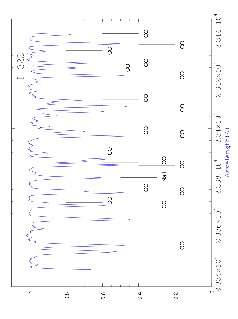
Figure 1: Observed spectrum in the K-band region of target star I-322. The selected CO molecular features (Table 2) are labelled, as well as the studied Na I line at 233379.137Å.

The spectra obtained are single order echelle with a resolution R=$\lambda$/$\Delta$$\lambda$=50,000 (corresponding to a resolution element of $\sim$ 4-pixels). The observations of the K-giants were obtained at two grating tilts, one in the K-band region ($\lambda$ $\sim$ 23,350 Å), and another in the H-band region ($\lambda$ $\sim$ 15,540 Å). Due to meteorological conditions, the M-giant targets were only observed in the H-band region. For those observations obtained in the K-band, spectra of hot stars were also needed for telluric division. The observed spectra were reduced to one-dimension by means of standard sets of IRAF routines (see Smith et al. 2002 for details). The typical S/N of the observed spectra is 100-200, with one star (IV-167) having a S/N = 50. A reduced Phoenix spectrum in the K-band region is shown in Figure 1 for target star IV-003; the prominent features appearing in the spectra, such as the numerous C¹² O¹⁶ lines and the Na I line are identified.

3 Analysis

The stellar parameters of effective temperature (T_eff) and surface gravity (parametrized as log g) are required for elemental abundance determinations. In addition, an estimate of the microturbulent velocity parameter, $\xi$, and the overall metallicity of the model atmospheres adopted in the calculations are needed.

3.1 Reddening, Photometric Colors, and Effective Temperatures

The spheroidal component of the Milky Way Galaxy has not been studied extensively due to the extremely high visual extinction ($\sim$ 30 mag) that affects its bulge. Even for target stars lying in Baade’s window, where there is significantly less extinction, it is challenging to obtain intrinsic (de-reddened) colors to an accuracy of $\sim$0.01 mag, which is needed in order to derive effective temperatures accurate to within 50K. Stanek (1996) constructed extinction and reddening maps for Baade’s window from color-magnitude diagrams obtained by the Optical Gravitational Lensing Experiment (OGLE; Udalski et al. 1993, 1994). These maps showed that extinction in Baade’s window is quite irregular, varying between 1.3 and 2.8 mag in A_v, with an estimated error of $\sim$ 0.1 mag. We used the extinction maps of Stanek (1996) and the A_v’s which are listed in Table 1 to derive the de-reddened colors for the targets stars (also in Table 1). The V magnitudes were taken from OGLE and the infrared magnitudes were taken from the 2MASS database.

In order to obtain effective temperatures for the K-giants, we adopted the Alonso et al. (1999) T_eff-calibrations for (J-K) and (V-K) colors, which are defined in the TCS (Telescopio Carlos Sanchez) system. The 2MASS colors for the target stars were transformed to the TCS system using the relations presented in Ramirez & Melendez (2005). Although the (V-K) calibration is considered one of the best T_eff indicators for cool stars (with an internal error estimated by Alonso et al. to be of $\sim$ 25K), the (V-K) color is also more sensitive to reddening, which represents a potential problem in bulge studies. On the other hand, the (J-K) color is less sensitive to reddening but the (J-K) T_eff-calibration has a larger internal error of $\sim$125 K (according to Alonso et al. 1999). Given these uncertainties, we adopted an average between the T_eff’s obtained from (J-K) and (V-K) calibrations as the final temperatures for the sample K giants. The average T(V-K) - T(J-K) for our sample is -48 $\pm$ 90K and we note that there is no trend with A_v.

The T_eff-calibrations adopted for the K-giants are not defined for the cooler giants of M spectral types. For the two M-giants in our sample we adopted the (J-K) calibration from Houdashelt et al. (2000). Transformations of the 2MASS colors to the CTIO system were needed, and we used the relations in Carpenter (2001). The Houdashelt et al. (2000) calibration has a small metallicity and log g dependance: for log g varying between 0.5 and 1.0 dex, (J-K) varies less than 0.02 mag. The calibration for log g=1.0 and [Fe/H]=0.0 are roughly coincident with the one for logg=0.5 and [Fe/H]=0.25. We adopted an average calibration for the parameter space between log g=0.5 and 1.0 (giant stars) and metallicities around solar (given that the target M giants have TiO bands and that very metal poor M-giants would not exist). Derived stellar parameters for target stars are presented in Table 1. As a consistency check we also estimated the effective temperature for the hotter M giant, BMB78, by means of the Bessel et al. (1998) calibration: this yields T_eff=3570 K, which is in good agreement with the value listed in Table 1.

3.2 Surface Gravities and Microturbulent Velocities

Classical determinations of spectroscopic log g’s rely on the forced agreement between the abundances obtained from Fe I and Fe II lines, typically, in the optical. Our observed infrared spectra do not contain adequate Fe lines in order to validate a purely spectroscopic determination. Surface gravities, however, can also be estimated from standard relations between stellar luminosity and mass. The log g’s in this study were estimated using the derived T_eff’s in Table 1 and the corresponding positions of the stars relative to isochrones computed by Girardi (2000), iterated for the final values of metallicities for each star. Since the bulge of the Milky Way is an old population we adopted the isochrones corresponding to 10 Gyr, and we note that age differences of several Gyrs will not have significant effects on the log g values for these old red-giants.

Microturbulent velocities ($\xi$) for giants can be estimated from the set of molecular CO lines which are present in the observed K-band spectra and that span a range in line strengths. Equivalent widths were measured for several CO lines (Table 2) and microturbulences for the K-giants were obtained from the requirement that the abundance is independant of the measured equivalent width. For the M-giants the microturbulences were estimated from the overall match between observed and synthetic spectra at 1.55 $\mu$m.

The adopted microturbulences (listed in Table 1) vary between $\xi$= 1.8 and 2.2 km/s for the K-giants; for the two M-giants in our sample we obtained $\xi$ = 2.5 and 3.0 km/s. These values are consistent with the trend of microturbulence versus the bolometric magnitudes (M_bol) and microturbulence versus log g’s found for Galactic M giants (Smith & Lambert 1985, 1986, 1990) and LMC red-giants (Smith et al. 2002). As discussed in Smith et al. (2005), the microturbulent velocities derived from infrared CO lines seem to be systematically higher than the ones typically obtained from Fe I lines in the optical. We note that the microturbulences derived here for the K-giant targets are also measurably larger than the values obtained from the Fe I lines in the optical by Fulbright et al. (2006) for the same stars; the average difference is 0.6 km s^-1. A comparison with the study by Rich & Origlia (2005) is not possible because the latter adopted a constant microturbulence of 2 km/s in their abundance analyses of M-giants.

3.3 Abundances

In the two wavelength intervals covered by the Phoenix spectra there are a number of CO, OH, and CN transitions, but only a few atomic absorption lines. We derived abundances of carbon, nitrogen and oxygen from molecular transitions of CO, CN and OH. In addition, we analyzed atomic lines from Na I, Ti I and Fe I. In order to derive the abundances we calculated synthetic spectra using the LTE synthesis code MOOG (Sneden 1973). All abundances were derived via spectrum synthesis, however, Table 3 displays the lines of OH, CN, Fe I, Na I and Ti I that were used for the abundance determinations. The molecular and atomic transitions analyzed in each case are discussed in the following section.

The model atmospheres used in the abundance calculations were interpolated from the original grid of MARCS models (BEGN, Gustafsson et al. 1975). The models were computed intially for metallicities ([Fe/H]) taken from Fulbright et al. (2006) and Rich & Origlia (2005). These metallicities were then adjusted until the metallicities of the models and the derived Fe abundances (from our sample Fe I infrared lines) were consistent. (The derivation of the Fe abundances from our infrared spectra will be discussed in the next section). A comparison of the model atmospheres adopted in this study, MARCS, with the more modern SOSMARCS (Plez, Brett & Nordlund 1992) indicates that differences in abundances are not significant (see Cunha et al. 2002).

3.3.1 Iron

Iron deserves discussion first as it is the fiducial element that is usually used as the primary ’metallicity’ indicator. The study here utilizes only IR spectra with limited wavelength coverage and iron is represented by a few well-defined Fe I lines near $\lambda$ 15530-15540 $\AA$ (Table 3). These Fe I lines are readily measurable in the Sun plus the well-studied K-giant $\alpha$ Boo. No laboratory measurements of oscillator strength exist for these lines but semi-empirical values are available from the Kurucz line list (Kurucz & Bell 1995), as well as solar gf-values from Melendez & Barbuy (1999).

In order to set the gf-values for Fe I lines, we measured equivalent widths from the disk-integrated solar spectrum from (Wallace et al. 1996) and used both Kurucz and Melendez & Barbuy (1999) gf-values to determine the solar photospheric iron abundance. Also, two solar models were used: one from the MARCS code and one from Kurucz ATLAS9 with T_eff=5777K, log g=4.438, and microturbulent velocity, $\xi$= 0.8 km/s. Note that the most recent photospheric abundance as reviewed by Asplund, Grevesse & Sauval (2005) is A(Fe)=7.45. The Fe I lines from Table 3 yield A(Fe)=7.31 $\pm$ 0.18 for the MARCS model and 7.37 $\pm$ 0.13 with the ATLAS9 model when Kurucz gf-values are used. We prefer to anchor our Fe analysis to a solar abundance of A(Fe)=7.45 with the MARCS model and adjusted the individual gf-values so that each line yielded 7.45 for A(Fe).

Given the solar gf-values defined above, an analysis of $\alpha$ Boo, using the spectra from Hinkle et al. (1996), provides a test of what Fe abundance these Fe I lines plus gf-values would yield for this well-studied K-giant. Examples of previous uses of $\alpha$ Boo in this role can be found, for example, in Smith et al. (2000) or Fulbright et al. (2006). Smith et al. derived T_eff=4300K log g=1.7, $\xi$= 1.6 km/s, and [M/H]=-0.60, while Fulbright et al. (2006) find T_eff=4290K, log g=1.55, $\xi$= 1.67 km/s, [M/H]=-0.50. The $\alpha$ Boo analysis used the same Fe I lines (and solar gf-values) that were adopted in this study of bulge red-giants, along with the model atmosphere as defined by Smith et al. (2000). The abundance results for $\alpha$ Boo are listed in Table 4: we find A(Fe) = 6.96 $\pm$ 0.05 ([Fe/H]=-0.49 $\pm$ 0.05). This value of [Fe/H] for $\alpha$ Boo is in excellent agreement with Fulbright et al. (2006) of [Fe/H]_αBoo=-0.49 $\pm$ 0.07, and suggests that our bulge Fe abundances scales can be compared directly at the low metallicity end.

3.3.2 Sodium and Titanium

In addition to Fe, as discussed in the previous section, there is a well-defined Ti I line at $\lambda$ 15543.720$\AA$ and one for Na I at $\lambda$ 233379.137Å. Both of these atomic lines are measurable in the Sun and we have (as with Fe I lines) derived solar gf-values using the 1D MARCS solar model with $\xi$=0.8 km s^-1 and A(Na)=6.17 and A(Ti)=4.90 (Asplund et al. 2005). These are the gf-values listed in Table 3.

With our derived solar gf-values the analysis of $\alpha$ Boo yields A(Na)=5.86 and A(Ti)=4.83 (Table 4), with both abundances in agreement with abundances from optical spectral lines. For example, Smith et al. (2000) find A(Na)=5.85$\pm$0.13 and A(Ti)=4.64 $\pm$ 0.12 based upon samples of optical lines of Ti I and Ti II. The agreement between optical and IR is excellent for Na and within the errors for Ti.

3.3.3 Carbon, Nitrogen and Oxygen

The observed spectra around $\lambda$23400$\AA$ contain a number of first overtone vibration rotation molecular CO lines. The selected CO lines are listed in Table 2, with the excitation potentials ($\chi$) and gf-values for the transitions taken from Goorvitch (1994). As discussed in Section 3.2, the sample CO lines were used to define the microturbulence parameter. We opted for measuring the equivalent widths of the CO lines (Table 2) and obtained estimates for the microturbulent velocities from the independance of CO abundances versus measured equivalent widths. We then computed synthetic spectra of the regions containing the sample CO lines for that derived microturbulent velocity. Fits to the observed profiles were obtained only from adjustments of the CO abundances; as expected the selected microturbulences were able to produce an overall good fit for strong and weak CO lines indicating that the adopted microturbulences and CO abundances were quite consistent with the results from synthetic fits of the entire CO spectral region.

The molecules of CO, OH, as well as CN, are abundant and important constituents of the molecular equilibrium in the atmospheres of cool stars; a consistent solution for the elemental abundances of carbon, nitrogen and oxygen has to be iterated until a good match between synthesies and observations is achieved for all of those spectral regions containing molecular transitions of CO, OH and CN, simultaneously. In order to obtain carbon and oxygen abundances we also synthesized, at the same time, the spectral region around 15540 Å, where there are 4 unblended lines of molecular OH. The atomic data for the OH transitions needed in order to construct a linelist for the synthesis were taken from Goldman et al. (1998) and the dissociation energy D₀ = 4.392 eV from Huber & Herzberg (1979) was adopted. A simultaneous solution was then obtained from the best fit to the observed spectra containing CO and OH, that defined the elemental carbon and oxygen abundances. Nitrogen abundances could then be obtained from weaker molecular CN lines molecular, which are present around 15540 Å, given that the carbon abundances are known. The line list adopted for the calculation of the synthetic spectra for the CN region was compiled B. Plez (private communication). The dissociation energy adopted is of 7.77 eV (Costes et al. 1990).

3.3.4 Final Abundances and Their Uncertainties

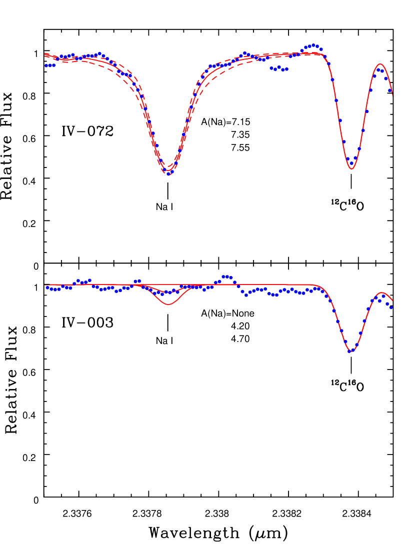
Figure 2: Observed and synthetic spectra for the two bulge giants in our sample which illustrate the large spread in Na abundances. We show Na I fits for one bulge target with a large Na abundance and another with sodium abundances much lower (close to an upper limit detection). The latter falls well below the trend of [Na/O] vs [O/H] defined by field stars in the Milky Way.

The atomic and molecular lines described in the previous three subsections were used, in conjunction with the stellar parameters, in Table 1 to derive the abundances listed in Table 4. Final abundances are presented for ¹²C, ¹⁴N, ¹⁶O, Na, Ti and Fe, all based upon spectrum synthesis. An example of spectrum sysnthesis of shown in Figure 2, which illustrates the Na I line in two bulge giants.

The S/N of the observed spectra is typically 100-200, with one star (IV-167) having a S/N = 50. From Cayrel’s (1988) formula, we estimate that the typical equivalent width uncertainty to range from $\sim$ 2 mÅ(e.g. for the CO line at 23367 Åin I-322 we measure an equivalent width of 384 mÅand the spectrum has a S/N=200) to 10 mÅ(for IV-167 with the lowest S/N in the sample) with a corresponding abundance uncertainty between 0.01 and 0.04 dex. These errors are much smaller than the abundance uncertainties caused by the errors in the stellar parameters themselves.

An analysis of the uncertainties in the abundances due to errors in the fundamental stellar parameters was conducted for each species. This analysis consisted of perturbing a representative star and analyzing it with different model atmospheres modified in Teff, log g, and $\xi$. In this case, the star IV-072 was used as the test and separate analyses were done for changes of $\delta$T=+75K, $\delta$log g=$\pm$0.25 and $\delta\xi$ = $\pm$ 0.3 km s^-1. The changes in the derived abundances for each element, as a function of each fundamental parameter are listed in Table 5. The final estimated error for each element is the quadrature sum of each uncertainty due to $\delta$T, $\delta$log g, and $\delta\xi$; this error is labeled $\Delta$ and is shown in the last column of Table 5. These errors dominate line-to-line scatter, in those cases where more than one of two lines are available (such as CO), thus uncertainties in the fundamental stellar parameters dominate the expected errors.

In addition to changing the stellar parameters independently, a simultaneous change in T_eff and log g is also investigated. This is because effective temperature and gravity are correlated along an isochrone, with log g decreasing if T_eff is decreased, for example. The last column of Table 5 quantifies this effect. Along these isochrones for old populations, a change of 75K in T_eff results in a change of about 0.15 dex in log g and it is these changes that are shown in the last column of Table 5. Again, IV-072 is used as the test and its basic model of T_eff=4400K and log g=2.4 is changed to T_eff=4325K and log g=2.25. This change results in a small change in $\xi$ as derived from the CO equivalent widths (from 2.2 to 2.1 km-s^-1) and the tabulated changes in the various elemental abundances. These changes are typical of what is found from the first exercise of changing the paramerters independently and the errors listed in Table 5 are approximately what is expected from an abundance analysis of this type.

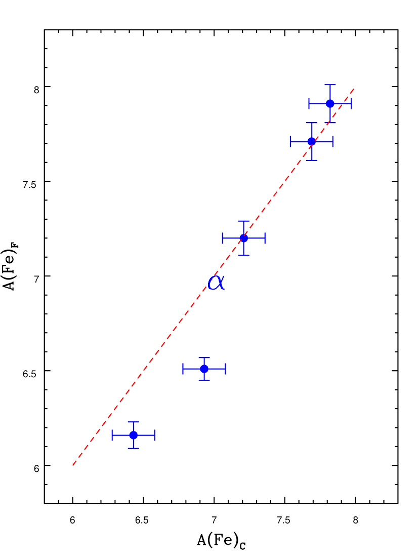
Figure 3: A comparison between the Fe abundances obtained for the 5 bulge K-giants in common with Fulbright et al. (2006) sample. The dashed line represents perfect agreement. The differences between the two studies are close to the expected uncertainties in each one, although there may be a metallicity dependent difference. We also show for compariosn the derived abundances in the two studies for the reference star Alpha Boo (represented by the $\alpha$ symbol; Table 4).

As discussed in Section 3.3.1 our Fe abundance scale is close to the scale of Fulbright et al. (2006). This comparison is illustrated in Figure 3 with Fe abundances plotted for the 5 bulge K-giants in common. The overall agreement is good, although there may be a slight metallicity dependant trend. The average difference and standard deviation $\Delta$A(Fe)(Us - Fulbright) = +0.11 $\pm$ 0.20. It is worth noting that our estimated errors in stellar parameters will cause an uncertainty of $\pm$0.12 dex in our Fe I abundances (Table 5). If this is combined with similar errors from Fulbright et al. (2006), the combined scatter will be $\pm$0.17 dex. One of the M-giants, BMB 289, was also in the Rich & Origlia (2005) study and four elemental abundances are in common: ¹²C, O, Ti and Fe. The average difference (Us - Rich & Origlia) and standard deviation of the two analyses of BMB 289 is $\Delta$=+0.08 $\pm$ 0.17. These differences can be considered to be within the expected uncertainties in the analyses.

4 Discussion

4.1 Carbon, Nitrogen and Mixing in the Bulge Red Giants

During stellar evolution along the red giant branch the abundance of carbon and nitrogen change due to the extensive convective envelope of the giant dredging material exposed to the CN-cycle to the spectroscopically observable surface. The main nuclei involved in the CN-cycle transmutations are ¹²C, ¹⁴N, and ¹³C (with ¹⁵N being a very minor constituent). This phase of stellar evolution has been labelled ’first dredge-up’, and extensively studied both observationally and theoretically. A simple sketch of first dredge-up would highlight the expectation that ¹²C nuclei are converted to mostly ¹⁴N, with some gain in the ¹³C abundance, and the ¹²C/¹³C ratio declines. If only the CN-cycle has operated significantly in the stellar matter the total number of C+N nuclei will be conserved, thus, as ¹²C is converted to ¹⁴N the ¹²C/¹⁴N will be lowered along a nearly predictable relation.

The target red giants are all evolved enough that they should have undergone some amount of first dredge-up. The combination of ¹²C and ¹⁴N abundances derived here can be used to quatify the consequence of first dredge-up. Conservation of C+N nuclei allows a check on the metallicity, i.e. Fe abundance, dependence of [C+N/Fe]. Ignoring ¹³C, a minor constituent, as we have no ¹³C information from the observed spectra, calculation of [¹²C+¹⁴N/Fe] reveals no upward or downward trend: ¹²C+¹⁴N scales as solar with Fe. The average [¹²C+¹⁴N/Fe]=0.00 $\pm$ 0.18 with the scatter of 0.18 dex being consistent within the uncertainties of combining three individual elemental abundances into one ratio.

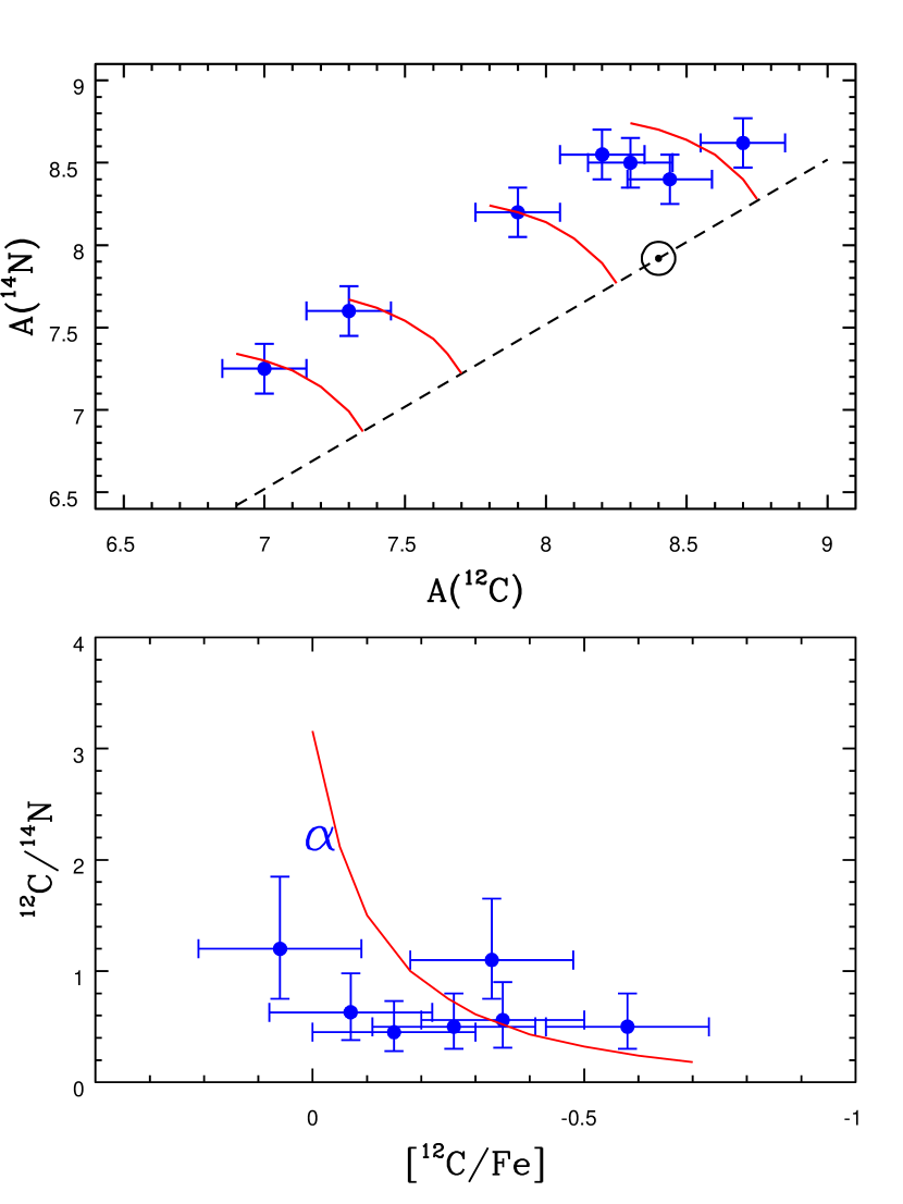
Figure 4: The top panel shows the nitrogen (A(¹⁴N)) versus carbon (A(¹²C)) abundances for the sample stars. The dashed line delineates the scaled solar line: all studied bulge red giants fall in the ¹⁴N-rich zone. The solid curves show lines of constant ¹²C+¹⁴N, or the so-called ’CN-mixing lines’. The bottom panel shows a CN-mixing curve normalized to the Fe abundance, so that all of the bulge red giants can be plotted with respect to a single curve. A solar ¹²C/¹⁴N=3.16 is taken as the initial value and declines as [¹²C/Fe] declines. Alpha Boo is also plotted (represented by the $\alpha$ symbol) with its ¹²C, ¹⁴N, and Fe abundances derived from the same lines as used for the bulge giants.

Evidence of the first dredge-up in the bulge red-giants is shown in Figure 4; the top panel plots A(¹⁴N) versus A(¹²C). The wavelength intervals observed in this study did not include measurable features with ¹³C, so the ¹²C/¹³C is not known. The solar point is plotted here with the solid straight line delineating [¹²C/Fe] and [¹⁴N/Fe] equal to 0.0. All of the studied bulge red giants fall above the scaled solar line, i.e., to the ¹⁴N-rich zone. The solid curves show lines of constant ¹²C+¹⁴N, or the so-called ’CN-mixing lines’. Although the ¹³C is not known, its maximum abundance due to H-burning will be only $\sim$1/3.5 that of ¹²C, which is itself depleted in mixed giants. The result of accounting for ¹³C in Figure 4 would flatten slightly the mixing curves as some ¹²C goes into ¹³C instead of ¹⁴N. Nevertheless, the mixing curves provide good approximations to what is observed in the bulge giants. Each of the three curves at the lower ¹²C abundances (for IV-003, IV329, and I-322) begin with initial ¹²C and ¹⁴N scaled by the respective Fe abundances. The most ¹²C- and ¹⁴N-rich mixing line begins an average Fe-abundance representative of the most metal-rich stars. The position of the bulge red giants is similar to what has been found for Galactic disk K and M giants (Smith & Lambert 1990) or even field M-giants in the LMC (see Figure 8 in Smith et al. 2002).

The ¹²C-depletion and ¹⁴N-enhancements are indicative of CN-cycle material. The conclusion of this investigation of the ¹²C and ¹⁴N abundances is that the ¹⁶O abundances in these bulge red giants are not measurably altered from their primordial values, as the mixing is not nearly extensive enough to have altered the initial ¹⁶O measurably.

The bottom panel of Figure 4 shows another view of CN-cycle mixing with all of the bulge giants scaled to a single mixing line. Here a solar ¹²C/¹⁴N=3.16 is taken as the initial value and this ratio declines as ¹²C is converted to ¹⁴N (or, as [¹²C/Fe] declines). The mixing curve is a reasonable approximation to the observed giants. Alpha Boo is also plotted with its ¹²C, ¹⁴N, and Fe abundances derived from the same lines as used for the bulge giants. This comparison bolsters confidence in the analysis and the interpretation that this sample of bulge stars are first dredge-up red giants.

4.2 The Oxygen Abundances and the Behavior of [O/Fe]

In red giants the C and N abundances are excellent monitors of dredge-up on the red giant branch. In old, low-mass red giants, such as the ones studied here, only the surface abundances of the isotopes of C and N, along with the minor oxygen isotopes ¹⁷O and ¹⁸O will be altered measurably by internal mixing. When studying low-mass giants it must be noted, however, that significant fractions of globular cluster giants do show ¹⁶O depletions that result from destruction by the higher temperature ON parts of the CNO cycles. The oxygen abundance variations are also observed in globular cluster turn-off and main-sequence stars (e.g. Gratton et al. 2001), thus the globular cluster O-variations arise from chemical evolution seemingly peculiar to them (Smith et al. 2005; Ventura & D’Antona 2005). The agreement in the bulge giants with the simple CN-mixing picture, as discussed in the previous section, demonstrates that the ¹⁶O abundances have not been altered measurably due to red giant dredge-up.

With confidence that the bulge red giant oxygen abundances represent the original values with which the star was born, they provide one of the key monitors of bulge chemical evolution. Oxygen has basically a single nucleosynthetic origin from massive stars and is produced over short timescales. As the iron yields from SN II are much less than oxygen, with Fe being synthesized most effectively in SN Ia over a significantly longer timescale, the ratio of O/Fe is the best indicator of SN II to SN Ia activity.

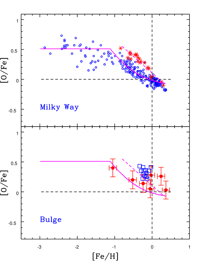
Figure 5: The behavior of [O/Fe] versus [Fe/H] for the Galactic disk and halo populations, along with the bulge. The top panel shows [O/Fe] from a number of studies (identified in the text) for halo and disk stars. The asterisks are specifically thick disk stars from Bensby et al. (2004) which are displayed in [O/Fe] relative to thin disk stars. The solid curve is a chemical evolution model for O and Fe yields from SN II and SN Ia, while the dashed line is a linear fit to the thick disk stars. The bottom panel illustrates [O/Fe] for bulge red giants. This study’s stars are shown as the large filled pentagons (with error bars) while the M-giants from Rich & Origlia (2005) are plotted as open squares. The galactic halo and disk curves from the top panel are also plotted as comparisons.

The Galactic disk and halo populations have had numerous published studies with [O/Fe] versus [Fe/H] and its overall behavior is fairly well-defined. This is illustrated in the top panel of Figure 5, with [O/Fe] taken from a number of studies (Edvardsson et al. 1993; Cunha, Smith & Lambert 1998; Melendez, Barbuy & Spite 2001; Smith, Cunha & King 2001; Melendez & Barbuy 2002; Fulbright & Johnson 2003). The asterisks in this figure are specific stars identified as thick disk stars from Bensby, Feltzing, & Lundstrom (2004). The decreasing values of [O/Fe] as [Fe/H] increase, for [Fe/H]$>$-1, is due to the increased Fe production from the onset of SN Ia. Below [Fe/H] of $\sim$ -1.0 all Galactic stars exhibit an elevated value of [O/Fe]. The simple exercise of combining oxygen and iron yields (with the caveat that the Fe yields are uncertain in the models) from the grid of models by Woosley & Weaver (1995), convolved with a standard IMF results in a value of [O/Fe]$\sim$+0.5: not very different from the observed halo values.

The beginning of the decrease in [O/Fe] in the Galactic halo occurs at roughly [Fe/H]=-1. The overall metallicity a population reaches (caused by SN II) when SN Ia’s begin to contribute to the chemical evolution is sensitive to the efficiency at which gas has been turned into stars. In this simple picture, the offset between the thin and thick disks in the [O/Fe]–[Fe/H] plane is caused by early, higher star formation rate in the thick disk, relative to the thin disk, with the result that the thick disk was more metal-rich by the time SN Ia’s began to explode. The solid curve in the top panel of Figure 5 is a simple numerical model of chemical evolution assuming no outflows or infalls and instantaneous recycling. The model has been adjusted to approximately follow the evolution from halo to thin disk. The thick disk stars from Bensby et al. (2004) are offset from this curve, with the dashed line a linear fit to the thick disk points.

Bulge values of [O/Fe] versus [Fe/H] are plotted in the bottom panel of Figure 5 and can be compared to the halo and disk populations. Red giants from this study are the large filled pentagon while the open squares are the recent Rich & Origlia (2005) M-giant abundances. The advantage of this study is the wider range in metallicity of targets, while the strong point of Rich & Origlia is the fairly large number of stars in a limited metallicity range (providing some limits on the intrinsic scatter in [O/Fe] in the bulge). At [Fe/H]$\sim$ -0.2 to 0.0, the [O/Fe] trend indicated by the abundances obtained here seems to be slightly lower (on average by 0.18 dex) than the results by Rich & Origlia (2005); within the uncertainties, however, the abundances in the two studies roughly overlap. The halo and thin disk model curve and the thick disk line are also plotted as references. The lowest-metallicity giant, IV-003 at [Fe/H]=-1.1, has a [O/Fe] value that is consistent with the Galactic halo. Among the more metal-rich bulge giants, there is a significant decline in [O/Fe] relative to star IV-003; the bulge population has undergone evolution in its O/Fe ratios. The decline in [O/Fe] in the bulge is not as large as for the thin disk, but is reminiscent of the thick disk trend. The most straightforward explanation of this trend is that the bulge underwent more rapid metal enrichment than the halo, but that star formation did continue over timescales that may include the onset of SN Ia.

4.3 Sodium in the Bulge

The chemical evolution of oxygen, the subject of the previous section, is dominated by SN II and its production is dependent on the mass function of its high-mass parent stars. One strong point of using oxygen to track the formation history of massive stars, with the subsequent dispersal of heavy elements and enrichment of the ISM, is that O-yields from SN II are not very sensitive to the progenitor-star metallicities. The integrated yields of oxygen are determined mostly by the shape of the stellar mass function: the ratios of very massive to less massive SN II.

Moving up the Periodic Table to study sodium provides different, and in some ways complementary insights into the details of chemical evolution. In most stellar populations studied to date Na is, like O, primarily a product of SN II (Clayton 2003). In globular clusters this may not be the case, but we will discuss the globulars later in this section. The key to sodium’s complementarity to an $\alpha$-element such as oxygen is that the yields of Na from SN II are quite sensitive to the inital SN II metallicities. The main source of Na is carbon-burning, but at the same time it can be destroyed at these temperatures by proton captures. The final yield from SN II thus depends on the p/n ratio, which is itself a function of metallicity, decreasing as the overall metallicity increases.

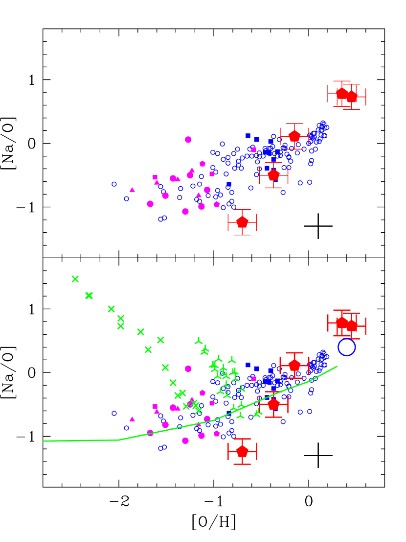
Figure 6: The behavior of Na and O in various stellar populations. Open circles are Galactic halo and disk results from many studies (noted in the text) while the small filled symbols represent Sculptor (circles), Carina (triangles), Fornax & Leo (pentagons), and the LMC (squares). This variety of stellar populations loosely define an increasing [Na/O] with [O/H]. An increasing Na/O yield with increasing oxygen is the qualitative prediction for SN II; model yields from Woosley & Weaver (1995) are added (the solid curve) in the bottom panel. Included in the bottom panel are abundances from the globular cluster M15 (4-point crosses) and M4 (3-point crosses); the Na-O anti-correlations are the signature of H-burning. The metal-rich open cluster NGC 6791 is also shown as the large open circle (from Peterson & Green 1998) and this metal rich point agrees with our most metal-rich bulge stars.

Figure 6 illustrates the behavior of Na and O in various stellar populations and betrays their origins by plotting [Na/O] versus [O/H]. The top panel shows results for field stars of the Milky Way halo, thick disk, and thin disk as small open circles, with these abundances from Reddy et al. (2003); Fulbright (2000); Fulbright & Johnson (2003); Nissen & Schuster (1997); Bensby, Feltzing & Lundstrom (2003); Prochaska et al. (2000). The small filled symbols show [Na/O] and [O/H] for the dwarf galaxies Sculptor (circles; Shetrone et al. 2003; Geisler et al. 2005), Carina (triangles; Shetrone et al. 2003), Fornax and Leo (pentagons; Shetrone et al. 2003), and the LMC (squares; Smith et al. 2002). There are two key points to the top panel: 1) all of the various populations overlap within the estimated errors of the many analyses (with the errors shown as representative errorbars), and 2) these diverse populations define a sequence of increasing Na/O with increasing metallicity (O/H). The scatter in [Na/O] at a given metallicity is not much larger, if at all, than the expected abundance uncertainties. The nearly unique relation of Na/O with O/H is dominated by SN II nucleosynthesis driving their evolution.

The large filled pentagons in the top panel of Figure 6 are the abundance results for the bulge stars. This sample includes a few quite metal-rich giants and provides values of [Na/O] at large [O/H], plus sample stars overlap with the less O-rich populations. In the overlap region of [O/H] the bulge stars agree well in [Na/O] versus [O/H] with the other populations. Near solar metallicity ([O/H] $\sim$ 0.0), the bulge stars overlap with the field-star sample but the lowest metallicity bulge star in our sample (IV-003) falls well below the trend. The Na I line in this star is very weak and the low Na abundance does not result from incorrect stellar parameters. (See the Na I synthesis in Figure 2.) Since the Na/O yields from SN II are metallicity sensitive, the low value of Na/O for IV-003 may indicate that the initial enrichment of the bulge to [O/H] $\sim$ -1 (or, [Fe/H] $\sim$ -1.3) was very rapid and dominated by very metal-poor massive stars (with [m/H] less than -2). This would be an example in which a metallicity-dependant ratio (Na/O) retained the metallicity signature of its parent SN II, regardless of how polluted the primordial cloud had become from the SN II (as measured by [O/H]). The field star trend, as defined by both the Milky Way halo and the dwarf galaxies, suggests a less efficient cycling of gas into stars when compared to the metal-poor tail of the bulge population. The trend defined by the highest metallicity bulge stars appears to be a smooth continuation from the lower metallicities. The overall behavior of Na/O is suggestive of SN II dominating the nucleosynthesis of Na in the bulge population.

In less massive stars than those that become SN II, Na production is possible via H-burning on the NeNa-cycle. This can occur at temperatures of a few to several times 10⁷K and one byproduct of this process can be ¹⁶O depletion due to the ON parts of the CNO-cycles. In the presence of significant contributions from NeNa- and CNO-cycles (as an explantion for the large Na abundances in the bulge) would be an expected anticorrelation of O and Na. The bottom panel of Figure 6 illustrates just such an effect where the same Galactic and dwarf galaxy field stars are plotted, as well as the bulge stars, with the addition of stars from two Galactic globular clusters (M13 and M4 as the 4-sided and 3-sided crosses, respectively). Here the H-burning signature is clear with the expected striking Na-O anticorrelations. No such trend is hinted at in this (admittedly small) bulge sample, indicating that chemical evolution in Na and O for the bulge has been driven largely by SN II.

In addition, in the bottom panel of Figure 6 we also show Na and O results for the metal-rich old open clusters NGC 6791 (Peterson & Green 1998) which agrees with the high sodium found here for the bulge targets. The solid curve plotted in this panel represents the Na and O yields from the SN II models of Woosley & Weaver (1995) convolved with a standard, i.e., Salpeter, mass function. The model curve is suggestive of the trend observed in the field stars, open clusters, and bulge stars and, within modest differences, points to SN II enrichment. It should be mentioned, however, that until more metal-rich SN II model yields are added to this plot, it may be that the most metal-rich bulge stars could show some contamination in Na and O from H-burning in a generation of intermediate mass stars. In addition, because the Bulge exhibits an abundance range in Fe, as well as a large variation in its Na/O values, it may show some similarities in the behavior of these 3 elements to that of the peculiar globular cluster $\omega$ Centauri (Norris & Da Costa 1995; Smith et al. 2000).

4.4 Titanium and the Behavior of [Ti/Fe] and [Ti/O] in the Bulge

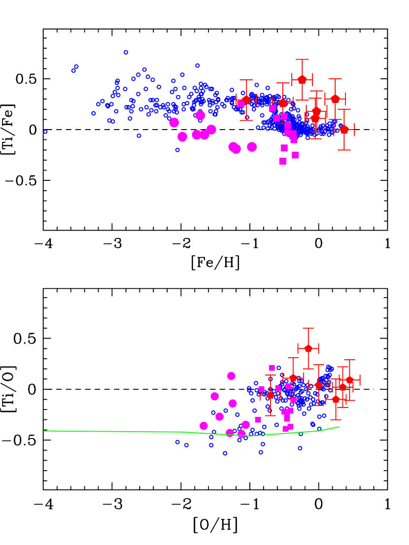
Figure 7: The top panel shows [Ti/Fe] versus [Fe/H] for different populations. The Galactic field stars shown as the small open symbols and are taken from a number of studies identified in the text. Other populations are also illustrated: large filled circles Sculptor (Shetrone et al. 2003; Geisler et al. 2005); large filled squares the LMC (Smith et al. 2002). The bulge stars are shown as the large filled pentagons (with error bars). As with [O/Fe], there is a tendency for the bulge values of [Ti/Fe] to remain elevated somewhat relative to the disk. The bottom panel shows the same stars as in the top panel but now plotted as [Ti/O] versus [O/H]. A general increase of [Ti/O] as [O/H] increases is seen as defined by all of the stellar populations. This increase is not predicted by the Woosley & Weaver (1995) yields that are shown as the solid curve in the bottom panel.

In the majority of stars studied in the Milky Way field halo and disk populations titanium behaves as an $\alpha$-element with respect to iron (e.g. see review by McWilliam 1997). This statement can be illustrated in Figure 7 (top panel) with [Ti/Fe] plotted versus [Fe/H] and the Galactic field stars shown as the small symbols. The Galactic results are taken from Gratton & Sneden (1988); Edvardsson et al. (1993); McWilliam et al. (1995); Prochaska et al. (2000); Carretta et al. (2002); Fulbright (2002); Johnson (2002); Bensby et al. (2003); Reddy et al. (2003). At metallicities with [Fe/H]$\leq$-0.6 to -0.8, [Ti/Fe] is elevated at a nearly constant plateau of $\sim$+0.3 dex. At increasing Fe abundances there is a rapid, perhaps even abrupt decline in [Ti/Fe] to near-solar ratios, with a roughly constant [Ti/Fe]$\sim$0.0 over [Fe/H]= -0.5 to +0.4.

Other populations are also illustrated in the top panel of Figure 7 with the large filled circles being Sculptor (Shetrone et al. 2003; Geisler et al. 2005) and the large filled squares the LMC (Smith et al. 2002). These two dwarf galaxies do not track the Galactic trend, with both smaller galaxies exhibiting the decline in [Ti/Fe] at lower values of [Fe/H] when compared to the Milky Way disk and halo fields. The bulge stars in Figure 7 are the large filled pentagons (plotted with error bars) and they define a somewhat different trend than any of the other populations. There is a tendancy of the bulge red giants to continue with elevated [Ti/Fe] values past the downturn shown by the halo-disk field stars (but the results presented here are based on a small number of 7 stars). The behavior of [Ti/Fe] as a function of [Fe/H] in the Bulge is reminiscent of that of [O/Fe]. The suggestion would be that the Bulge underwent a more rapid metallicity enrichment from SN II than the halo, but in the most metal-rich bulge stars there is a decline in [$\alpha$/Fe] (found in our sample for both O and Ti).

The bottom panel of Figure 7 shows the same stars as in the top panel but now plotted as [Ti/O] versus [O/H]. As in Figure 6, replacing Fe with O in the comparisons removes to some approximation the role of SN Ia and focusses on the role of SN II. As in the comparison of [Na/O] versus [O/H], the various stellar populations now fall along a similar trend, in this case one of an increase of [Ti/O] as metallicity, i.e. [O/H], increases. This behavior was not expected based on the SN II model yields, which are plotted in this panel as the solid curve. This curve is defined by the Woosley & Weaver (1995) yields convolved with a Salpeter mass function at each metallicity. Given the large number, and varied natures of the studies plotted here, the scatter in [Ti/O] at a given [O/H] is not large ($\sim$$\pm$0.25 dex). The lower-metallicity bulge stars studied here fall right in the trend defined by the Galactic halo-disk field stars. The metal-rich bulge stars continue as an extension of this trend. The small cluster of metal-rich disk stars (with [O/H]$>$0.0) are from Bensby et al. (2003) and agree well with the metal-rich bulge stars.

Titanium is a product of explosive Si-burning, probably as a result largely of SN II, with the dominant ⁴⁸Ti isotope derived from the production and subsequent decay of ⁴⁸Cr. The smooth trend defined by the populations of Sculptor, the LMC, the Galactic field stars, and the bulge all point to one source and would suggest SN II. We offer no explanation for the trend in [Ti/O] but point out the significant trend in [Ti/Si] as a function of galactocentric distance in Galactic globular clusters noted by Lee and Carney (2002).

5 Conclusions

$\bf Iron$: Our bulge sample, although admittedly small, spans a significant range across the metallicity distribution as found from low resolution studies of the bulge. The sampled metallicity range thus provides the opportunity to infer characteristics of bulge chemical evolution as defined by the abundances summarized below.

Carbon, Nitrogen and the CN cycle: The ¹²C-depletion and ¹⁴N-enhancements are indicative of CN-cycled material. The conclusion of this investigation into the ¹²C and ¹⁴N abundances is that the ¹⁶O abundances in the studied bulge red giants are not measurably altered from their primordial values, as the mixing is not nearly extensive enough to have altered the initial ¹⁶O measurably. Therefore, the derived oxygen abundances represent good monitors of chemical evolution within the bulge population.

$\bf Oxygen$ : At low metallicity, the [O/Fe] results agree with halo-like [O/Fe] abundances. The [O/Fe] values then decline as [Fe/H] increases. The decline in [O/Fe] in the bulge, however, is not as large as for the thin and thick disk at the highest metallicities. The most straightforward explanation of this trend is that the bulge underwent more rapid metal enrichment than the halo, but that star formation did continue over timescales that may include the onset of SN Ia.

$\bf Sodium$: Near solar metallicity ([O/H] $\sim$ 0.0), the bulge stars overlap the field-star distributions but the lowest metallicity bulge star in our sample (IV-003) falls well below the trend. Since the Na/O yields from SN II are metallicity sensitive, the low value of Na/O for IV-003 may indicate that the initial enrichment of the bulge to [O/H] $\sim$ -1 was quite rapid and dominated by very metal-poor massive stars (with [m/H] less than -2). This would be an example in which a metallicity-dependant ratio (Na/O) retained the metallicity signature of its parent SN II. At the highest metallicities, the sodium abundances are very high, defining a sharp upward trend with the oxygen abundance. It is interesting to note that this pattern of high sodium was also found for the metal rich open cluster NGC 6791 by Peterson & Green (1998).

$\bf Titanium$: The Ti abundances obtained define a somewhat different trend than any of the other populations in the Milky Way. There is a tendancy of the bulge red giants to retain elevated [Ti/Fe] values past the downturn shown by the halo-disk field stars. In addition, the bulge stars are significantly more elevated relative to [Ti/Fe] versus [Fe/H] in dwarf spheroidals. The behavior of [Ti/Fe] as a function of [Fe/H] in the bulge is reminiscent of that of [O/Fe]. The suggestion would be that the bulge underwent a more rapid metallicity enrichment from SN II than the halo, but in the most metal-rich bulge stars there is a decline in [$\alpha$/Fe] (found in our sample for both O and Ti).

6 Acknowledgements

We thank Jon Fulbright, Vanessa Hill, Manuela Zoccali and Dante Minniti for helpful discussions. Based on observations obtained at the Gemini Observatory, which is operated by the Association of Universities for Research in Astronomy, Inc., under a cooperative agreement with the NSF on behalf of the Gemini partnership: the National Science Foundation (United States), the Particle Physics and Astronomy Research Council (United Kingdom), the National Research Council (Canada), CONICYT (Chile), the Australian Research Council (Australia), CNPq (Brazil), and CONICRT (Argentina), as program GS-2004A-Q-20. This paper uses data obtained with the Phoenix infrared spectrograph, developed and operated by the National Optical Astronomy Observatory. This work is also supported in part by the National Science Foundation through AST03-07534 (VVS), NASA through NAG5-9213 (VVS), and AURA, Inc. through GF-1006-00 (KC).

Table 1: Stellar Quantities & Parameters

Star	AV	V0	J0	K0	Teff(K)	Log ga	$\xi$ (km s-1)
I-322	1.48	13.01	10.75	9.93	4250	1.5	2.0
IV-003	1.30	13.70	11.75	11.03	4500	1.3	1.8
IV-167	1.46	15.59	13.45	12.67	4375	2.5	2.2
IV-072	1.46	14.93	12.73	11.99	4400	2.4	2.2
IV-329	1.35	13.81	11.54	10.73	4275	1.3	1.8
BMB 78	1.35	–	8.52	7.38	3600	0.8	2.5
BMB 289	1.62	–	7.29	5.98	3375	0.4	3.0

Note. — (a): Units of cm s^-2.

Table 2: ¹²C¹⁶O Lines and Equivalent Widths^a for K-giants

$\lambda$(Å)	$\chi$(eV)	Log gf	I-322	IV-003	IV-072	IV-167	IV-329
23350.777	0.42	-5.084	579	302	590	—	—
23367.117	0.01	-6.338	384	86	394	610	275
23368.221	2.15	-4.780	86	54	73	69	75
23372.385	0.40	-5.124	—	260	506	508	405
23373.398	1.66	-4.456	—	113	244	218	189
23383.809	0.39	-5.146	527	244	—	525	394
23385.273	1.69	-4.447	—	69	237	255	194
23386.213	0.00	-6.438	—	112	332	302	242
23388.523	2.20	-4.772	96	—	—	—	—
23395.646	0.38	-5.167	547	255	517	448	382
23397.609	1.73	-4.439	350	62	—	180	158
23407.893	0.36	-5.190	535	234	507	620	387
23410.404	1.76	-4.431	247	50	303	380	161
23420.557	0.35	-5.214	510	—	—	462	440
23423.668	1.80	-4.421	252	—	278	285	196
23425.664	0.00	-6.745	307	—	222	225	215
23430.629	2.29	-4.757	79	—	—	—	—
23433.635	0.35	-5.240	520	—	460	—	411
23437.393	1.84	-4.414	—	—	268	268	—

Note. — (a): Equivalent widths in mÅ.

Table 3: Lines used as Abundance Indicators via Spectrum Synthesis

$\lambda$(Å)	$\chi$(eV)	log gf
Fe I
15531.742	5.64	-0.564
15531.750	6.32	-0.900
15534.239	5.64	-0.402
15537.572	5.79	-0.799
15537.690	6.32	-0.660
Na I
23378.945	3.75	-0.420
23379.139	3.75	+0.517
Ti I
15543.720	1.88	-1.481
12C14N
15530.987	0.89	-1.519
15544.501	1.15	-1.146
15552.747	0.90	-1.680
15553.659	1.08	-1.285
15563.376	1.15	-1.141
16OH
15535.489	0.51	-5.233
15560.271	0.30	-5.307
15568.807	0.30	-5.270
15572.111	0.30	-5.183

Table 4: Abundances^a

Star	A(12C)	A(14N)	A(160)	A(Na)	A(Ti)	A(Fe)
I-322	7.90	8.20	8.60	6.13	5.15	7.21
IV-003	7.00	7.25	8.05	4.23	4.14	6.40
IV-072	8.70	8.62	9.20	7.35	5.44	7.69
IV-167	8.44	8.40	9.10	7.30	5.27	7.82
IV-329	7.30	7.60	8.35	5.30	4.64	6.93
BMB78	8.30	8.50	9.00	–	5.05	7.42
BMB289	8.20	8.55	8.75	–	4.94	7.40
Arcturus	7.92	7.60	8.49	5.85	4.83	6.96

Note. — (a): A(X)= log[n(X)/n(H)] + 12. The solar iron abundance is A(Fe)_⊙= 7.45.

Table 5: Abundances Errors due to Stellar Parameter Uncertainties

Element	$\delta$T=+75K	$\delta$log g=+0.25	$\delta\xi$=+0.3km s-1	$\Delta^{a}$	$\delta$T + $\delta$log g b
12C	+0.05	+0.12	-0.08	$\pm$0.15	-0.12
14N	+0.08	+0.10	-0.06	$\pm$0.14	-0.17
16O	+0.12	+0.12	-0.03	$\pm$0.17	-0.19
Na	+0.10	+0.01	-0.02	$\pm$0.10	-0.13
Ti	+0.12	+0.02	-0.09	$\pm$0.15	-0.10
Fe	+0.01	+0.05	-0.11	$\pm$0.12	-0.01

Note. — (a): [($\delta T)^{2}$ + ($\delta$log g)² + ($\delta\xi)^{2}$]^1/2

Note. — (b): Simultaneous change in $\delta$ T=-75K and $\delta$log g=-0.15. This changed $\xi$ from 2.2 to 2.1 km/s.

References

- (1) Alonso, A, Arribas, S. & Martinez-Roger, C. 1999, A&A Supp. 140, 261
- (2) Asplund, M., Grevesse, N., & Sauval, A. J. 2005 In Cosmic Abundances as Records of Stellar Evolution and Nucleosynthesis, ed. F. N. Bash, & T. G. Barnes p. 25
- (3) Baade, W. 1944, ApJ, 100, 137
- (4) Bensby, T., Feltzing, S., & Lundstrom, I. 2003, A&A, 410, 527
- (5) Bensby, T., Feltzing, S., & Lundstrom, I. 2004, A&A, 415, 155
- (6) Bessel, M.S., Castelli, F., & Plez, B. 1998, A&A, 333, 231
- (7) Cayrel, R. 1988, in IAU Symp. 132, The Impact of Very High S/N Spectroscopy on Stellar Physics, ed. R. Cayrel, G. de Strobel & M. Spite (Dordrecht: Kluwer), 354
- (8) Carpenter, J. M. 2001, ApJ, 121, 2851
- (9) Carretta, E., Gratton, R., Cowan, J.G., Beers, T.C. ,& Cristlieb, N. 2002, AJ, 124, 481
- (10) Clayton, D. 2003, Handbook of Isotopes in the Cosmos (Cambridge University Press: Cambridge)
- (11) Costes, M., Naulin, C., & Dorthe, G. 1990, A&A, 232, 270
- (12) Cunha, K., Smith, V., & Lambert, D. L. 1998, ApJ, 493, 195
- (13) Cunha, K., Smith, V. V.; Suntzeff, N. B.; Norris, J. E.; Da Costa, G. S.; Plez, B. 2002, AJ, 124, 379
- (14) Edvardsson, B., Andersen, J., Gustafsson, B., Lambert, D. L., Nissen, P. E., & Tomkin, J. 1993, A&A, 275, 101
- (15) Fulbright, J. P. 2000, AJ, 120, 1841
- (16) Fulbright, J. P. 2002, AJ, 123, 404
- (17) Fulbright, J. P. & Johnson, J.A. 2003, ApJ, 595, 1154
- (18) Fulbright, J., McWilliam, A., & Rich, M. R. 2006 ApJ, 636, 821
- (19) Girardi, L. Bressan, A. Bertelli, G., & Chiosi, C. 2000, A&AS, 141, 371
- (20) Geisler, D., Smith, V. V., Wallerstein, G., Gonzalez, G. & Charbonnel, C. 2005, AJ, 129,1428
- (21) Goldman, A., Shoenfeld, W. G., Goorvitch, D., Chackerian, C. Jr., Dothe, H., Melen, F., Abrams, M.C., & Selby, J. E. A. 1998, J. Quant. Spectrosc. Radiat. Transfer 59, 453
- (22) Goorvitch, D. 1994, ApJS, 95, 535
- (23) Gratton, R. G., & Sneden, C. 1988, A&A, 204, 193
- (24) Gratton, R. G., Bonifacio, P., Bragaglia, A., Carretta, E., Castellani, V., Centurion, M., Chieffi, A., Claudi, R., Clementini, G., D’Antona, F., and 9 coauthors 2001, A&A, 369, 87
- (25) Gustafsson, B., Bell, R. A., Eriksson, K., & Nordlund, A. 1975, A&A, 42, 407
- (26) Hinkle, K. H., Wallace, L., & Livingston, W. 1995, Infrared Atlas of the Arcturus Spectrum, 0.9–5.3Zm (San Francisco:ASP)
- (27) Hinkle et al. 2003, Proc. SPIE, 4834, 353
- (28) Houdashelt, M. L., Bell, R. A., & Sweigart, A. V. 2000, AJ, 119, 1448
- (29) Huber, K-P, & Herzberg, G. 1979, Constants of Diatomic Molecules (New York: Van Nostrand)
- (30) Johnson, J. A. 2002, ApJS, 139, 219
- (31) Kurucz, R. & Bell, R. 1995, Atomic spectral line database from CD-ROM 23
- (32) Lee, J., & Carney, B. W. 2002, AJ, 124, 1511
- (33) McWilliam, A. & Rich, R. M. 1994, ApJS, 91, 749
- (34) McWilliam, A., Preston, G. W., Sneden, C., Searle, L. 1995, AJ, 109, 2757
- (35) Melendez, J. & Barbuy, B. 1999, ApJS, 124, 527
- (36) Melendez, J. & Barbuy, B. 2002, ApJ, 575, 474
- (37) Melendez, J. & Barbuy, B., & Spite, F. 2001, ApJ, 556, 858
- (38) Nissen, P.E., & Schuster W.J 1997, A&A, 326, 751
- (39) Nissen, P.E., Primas, F., Asplund, M., & Lambert, D. L. 2002, A&A, 390, 235
- (40) Norris, J. E., & Da Costa, G. S. 1995, ApJ, 447, 680
- (41) Peterson, R. C., & Green, E. M. 1998, ApJ, 502, L39
- (42) Prochaska, J. X., Naumov, S. O., Carney, B. W., McWilliam, A., Wolfe, A. M. 2000, AJ, 120, 2513
- (43) Plez, B., Brett, J.M. & Nordlund, A. 1992 A&A, 256, 551
- (44) Ramirez, I. & Melendezi, J. 2005, ApJ, 626, 465
- (45) Reddy, B. E., Tomkin, J., Lambert, D. L., & Allende Prieto, C. 2003, MNRAS, 340, 304
- (46) Rich R. M. & Whitford, A. E. 1983, ApJ, 274, 723
- (47) Rich, R. M. 1988, AJ, 95, 828
- (48) Rich, R. M. 1990, ApJ, 362, 604
- (49) Rich, R. M. & Origlia, L. 2005, ApJ, 634, 1293
- (50) Sadler, E. M., Rich, R. M.,& Terndrup, D. M. 1996, AJ, 112, 171
- (51) Shetrone, M., Venn, K. A., Tolstoy, E., Primas, F., Hill, V., Kaufer, A. 2003, AJ, 125, 684
- (52) Sneden, C. 1973, ApJ, 184, 839
- (53) Smith, V. V. & Lambert, D. L. 1985, ApJ, 303, 226
- (54) Smith, V. V. & Lambert, D. L. 1986, ApJ, 311, 843
- (55) Smith, V. V. & Lambert, D. L. 1990, ApJS, 72, 387
- (56) Smith, V. V., Suntzeff, N. B., Cunha, K., Gallino, R., Busso, M., Lambert, D. L., Straniero, O 2000, AJ, 119, 1239
- (57) Smith, V. V., Cunha, K., & King, J. R. 2001, AJ, 122, 370
- (58) Smith, V. V., Hinkle, K. H., Cunha, K., Plez, B., Lambert, D. L., Pilachowski, C. A., Barbuy, B., Melendez, J., Balachandran, S., Bessel, M. S., Geisler, D. P., Hesser, J. E., & Winge, C., 2002, AJ, 124, 3241
- (59) Smith, V. V., Cunha, K., Ivans, I., Lattanzio, J. C.; Campbell, S., Hinkle, K. H. 2005, ApJ, 633, 392
- (60) Stanek, K. Z. 1996, ApJ, 460, L37
- (61) Terndrup, D. M., Sadler, E. M., & Rich, R. M. 1995, AJ, 110, 1774
- (62) Udalski, A.; Szymanski, M.; Kaluzny, J.; Kubiak, M.; Mateo, M. 1993, Acta Astron., 43, 69
- (63) Udalski, A.; Szymanski, M.; Stanek, K. Z.; Kaluzny, J.; Kubiak, M.; Mateo, M.; Krzeminski, W.; Paczynski, B.; Venkat, R. 1994, Acta Astron., 44, 165
- (64) Ventura, P., & D’Antona, F. 2005, ApJ, 635, L149
- (65) Wallace, L.; Livingston, W.; Hinkle, K.; Bernath, P. 1996, ApJS, 106, 165
- (66) Woosley, S. E., & Weaver, T. A. 1995, ApJS, 101, 181