Detecting Irregular Orbits in Gravitational N-body Simulations

Abstract

We present a qualitative diagnostic based on the continuous wavelet transform, for the detection of irregular behaviour in time series of particle simulations. We apply the method to three qualitatively different gravitational 3-body encounters. The intrinsic irregular behaviour of these encounters is well reproduced by the presented method, and we show that the method accurately identifies the irregular regime in these encounters. We also provide an instantaneous quantification for the degree of irregularity in these simulations. Furthermore we demonstrate how the method can be used to analyze larger systems by applying it to simulations with 100-particles. It turns out that the number of stars on irregular orbits is systematically larger for clusters in which all stars have the same mass compared to a multi-mass system. The proposed method provides a quick and sufficiently accurate diagnostic for identifying stars on irregular orbits in large scale $N$-body simulations.

1 Introduction

Gravitational $N$-body systems are intrinsically chaotic, at least for $N>2$ [1]. For $N=2$ Newtonian systems are regular, but post Newtonian dynamics[2, 3, 4] can already reveal chaotic behaviour [5, 6] by $N=2$. Chaoticity in a self gravitating systems with $N>2$ can reveal itself on a very short time scales, of the order of orbital periods. On the other hand, in some systems like the planetary system around the Sun, chaoticity only reveals itself on a time scale of billions of orbits [7, 8]. In a stellar cluster which does not contain a dominant central mass, orbits can be chaotic on a much smaller time scale. In such an environment seemingly regular orbits can suddenly become highly irregular, to return later to regular again [9, 10].

In this study we focus on the characterisation of orbits which show irregular behaviour on a short (dynamical) time scale, and not on a long (relaxation) time scale. Star clusters, with contain between about 100 and O($10^{7}$) stars, are governed by microscopic few body interactions [11]. Analysis of such systems is often hampered by this internal microscopic physics and a qualitative indicator of chaotic behaviour could enormously assist in the understanding of large scale gravitational $N$-body simulations. In particular, since it is thought that stars on irregular orbits in self gravitating $N$-body systems have an important effect of the bulk properties of such systems [12].

We present a transparent diagnostic to qualify chaotic behaviour of individual trajectories in $N$-body systems. In addition, the method has some quantitative qualities. The application of this method ranges from 3-body interactions to simulations of entire star clusters and galaxies. For clarity, we define irregular orbits as orbits which are deterministic though sensitive to the initial conditions and which cannot be described as a sum of periodic motions.

The motion of a star in an N-body simulation can change from regular to irregular (and vice versa) due to gravitational interactions with other stars. Irregularity of an orbit then is a local quantity, and this forces us to deviate from the conventional methods based on Lyapunov [13] numbers such as explained in [14, 15, 16]. In addition, the calculation of Lyapunov exponents is costly, may require reruns and are therefore less suited for a direct diagnostic, whereas we are predominantly interested in a diagnostic that can be evaluated at runtime. The Lyapunov indicator, however, is well suited for discriminating between ordered and weak chaotic motion, like planetary systems, whereas we are in particular interested in very chaotic systems [14]. Others methods for detecting chaos in Hamiltonian systems, such as SALI [17, 18], Fourier Transform [19, 20, 21], Poincaré Section [22], the zero-one method [23] and the geometric indicator [24] are also less suited for analysing gravitational $N$-body simulations during run time, since they also are not practical in providing an instantaneous quantification of the chaoticity of the system we are interested in here.

In § 2 we discuss the basics of the Continuous Wavelet Transform (CWT), which we present in a package called CWaT. We then proceed by applying this method to several N-body simulations in § 3, to conclude in § 4.

2 Method for detecting chaos

2.1 The continuous wavelet transform

The continuous wavelet transform [25] (CWT) gives the time-frequency representation of a time series $f(t)$ by fitting a wavelet $\Psi$ to it at subsequent points in time $t$. We have used the Morlet-Grossmann wavelet [26], which is described by

$$\Psi(t)=e^{i\omega_{0}t}e^{{-t^{2}}/{2\sigma^{2}}}.$$ (1)

Here $\sigma$ is a measure of the spread in time and $\omega_{0}$ the base frequency of the wavelet. The wavelet is a periodic sinusoidal signal enveloped by a Gaussian, from which we can construct a family of wavelets using a scaling factor $\alpha$ and a time shift $\beta$

$$\Psi_{(\alpha,\beta)}(t)=\frac{1}{\alpha}\Psi\left(\frac{t-\beta}{\alpha}\right),\qquad\quad\beta\in\mathcal{R},\qquad\quad\alpha>0.$$ (2)

We define the CWT as

$$T(\alpha,\beta)=\int\limits_{-\infty}^{\infty}{f(t)\overline{\Psi}_{(\alpha,\beta)}(t)dt}.$$ (3)

Here $\overline{\Psi}$ is the complex conjugate of $\Psi$ and $f(t)$ a time series. Fitting the wavelet to $f(t)$ at discrete moments in time ($\beta\in[0,t]$) yields $T(\alpha,t)$. We express $T(\alpha,t)$ in terms of frequency $\omega$ rather than scale $\alpha$ (since we are more accustomed to the former) using the relation

$$\omega=\frac{\omega_{0}}{\alpha}.$$ (4)

This leads to a time-frequency representation $T(\omega,t)$. For an extensive discussion see [27].

2.2 Analysing the CWT

The main features of the time series can be described by its instantaneous frequencies $\omega(t)$. These can be extracted from $T(\omega,t)$ by selecting its local maxima. We only consider all local maxima larger than a threshold $\tau=0.95$ of the global maximum. In this we take a different approach than [28, 29] who explicitly consider the global maximum. Using a lower threshold enables us to filter most of the noise from the CWT without losing the relevant information on which the $\chi$ can be determined. We also tried $\tau=0.93$ and $\tau=0.97$, which gave very similar results in the resulting value of $\chi$.

We find the extrema by simulated annealing [30, 31], following [32]. Connecting the local maxima results in a number of curves in the time-frequency domain, which we call ridges. The time series is subsequently analysed by studying the ridges, enabling a qualitative analysis of the behaviour of the time series. This is considerably more practical than using the CWT directly, an example is presented in fig.  2.

A periodic time series (i.e. with a constant frequency) results in a uninterrupted horizontal ridge indicating the fundamental frequency $P$ and possibly overtones spaced at periods $P/n$ where $n$ is integer. A quasi-periodic time-series can be described by a sum of periodic time series, each with its own ridge at a specific frequency. Such a time series is then represented by multiple horizontal ridges. Irregular time series on the other hand lead to curved ridges of limited length [33].

2.3 A quantitative measure of chaos

To bring the chaos detecting qualities of the method one step further we quantify the number of ridges and their curvature in the irregularity indicator $\chi$. We define $\chi$ at any moment in time by:

$$\chi(t)=\frac{1}{n(t)}\sum\limits_{i=1}^{n(t)}\left|s_{i}\right|.$$ (5)

Here $n(t)$ is the number of ridges at time $t$ and $s_{i}$ a measure for the slope of ridge $i$. Using a least squares fit we calculate the slope of the ridge. Because $\chi$ would be dominated by large values of the slope we use an empirical cutoff. The slope is normalised to unity to assure that $s_{i}\in[0,1]$.

The ridges of periodic and quasi-periodic time series are represented by horizontal ridges, they imply $\chi(t)\simeq 0$ (see § 2.2). We note however that the proposed indicator (see Eq.  5), cannot give a yes/no definition about the occurrence of local exponential instability, but it is capable of giving a measure of the degree of instability.

3 Application

To demonstrate the effectiveness of CWaT we apply it to three gravitational 3-body interactions. Such interactions are irregular [34], with some regular characteristics (see [35, 36] for an interesting earlier analysis of this sort).

In each of the three following examples we inject a single object (star) in a system consisting of two objects (stars) which are bound in a binary. A time series is constructed by projecting the orbit of each of the stars on three orthogonal axes (see also [19]). The stellar orbits are computed using the starlab software environment [37, 38] which is publicly available from
http://www.ids.ias.edu/~starlab. This $N$-body integration package calculates the orbits of the stars with individual time steps [39] using a fourth-order Hermite predictor-corrector scheme [40]. A regular time series is constructed by Hermite interpolation at evenly spaced time intervals. The time step adopted for CWT is $1/1024^{\rm th}$ of the total integration time. Further analysis is carried out with the S-WAVE software package [32], to ultimately calculate the CWT and the ridges of the time series.

In the following two §§  we discuss the chaotic behaviour in one non-resonant preserving encounter and one resonant encounter. In the first encounter the incoming star escapes after a close encounter with a binary. In the following example, in § 3.2 (see [41] for more examples, and even some very peculiar orbits in [42]), the incoming star has multiple close interactions with the binary, we call such interactions ‘resonant’. The example shown is a democratic resonance which is characterised by all three stars interacting strongly with multiple close passages; each star generally interacts with comparable frequency with any of the other stars.

We use the following convention: star #1  and #2  form the initial binary which is encountered by star #3. The time series give the position of the star with respect to the centre of mass of the 3-body system. The units are given in standard N-body units [43].

3.1 Irregular motion in a non-resonant gravitational interaction

In the first example we select an interaction between a binary, consisting of star #1  and #2  to interact with a single incoming star, #3. After interacting with the binary, star #3  escapes without disrupting the binary. The incomer, however, may change the binding energy of the binary. Precise initial conditions are presented in Tab. 1.

In fig. . 1 we present a schematic diagram of the interaction. In this example the binary has a close encounter with the incomer at $t\simeq 150$. After the encounter the incoming star is deflected along a hyperbolic path.

The analysis using CWaT of one of the nine (three stars and three axes) time series is given in fig. 2. The top panel shows the time series of the position of star #2  projected on the $y$-axis in N-body spacial coordinates versus N-body time units. In the first $150$ N-body time units, $t=[0,150]$, the binary moves upward (in $y$) with respect to the centre of mass because the incomer (star #3) is approaching it from above. The projection of the circular motion results in the sinusoidal behaviour of the time series. The motion of the binary with respect to the centre of mass is downwards after the encounter with the incomer.

The second panel of fig.  2 shows $T(\omega,t)$. Its most prominent feature is two arch-like shapes in the period region 10 to 100 spanning $t=[30,150]$ and $t=[150,330]$. These arches are the sum of one arch spanning $t=[30,330]$ due to boundary effects [44] and a triangular feature centred at $t\simeq 150$ due to the centre of mass motion of the binary. These regions of high intensity result in ridges with periods $P\simeq 86$ and $P\simeq 61$ in the third panel.

The ridge at $P\simeq 6.3$ in the third panel indicates the period of the binary system, which after $t\simeq 150$ has reduced to $P\simeq 6.0$. This ridge is joined by another on the interval $t=[150,330]$ at a shorter period of $P\simeq 3$. The lower period ridge is an overtone caused by an increase of the eccentricity of the binary from $e=0$ to $e\simeq 0.38$.

As we discussed in Section 2.3, the bottom panel of fig.  2, shows that $\chi\simeq 0$ during the entire interaction in accordance with the periodic behaviour of the system. The short fly-by interaction has not let to a qualitative indication of irregular behaviour in the system.

A similar analysis can be performed for any star and for each projection. The result will be quite similar, supporting the argument that the presented method is independent of the selection of a fundamental plane.

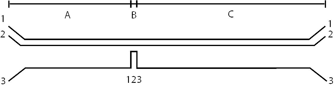
Figure 1: Schematic representation of a non-resonant three body interaction. The interacting stars on the left are indicated by 1, 2 and 3, each of which progresses in time along the solid curve to the right. Initially star 1 and 2 are close together, as is also indicated in the representation. A close encounter with star 3 sometime half way the encounter is marked by the three lines coming close together. The label “$123$” identifies the moment of closest approach between the three stars. To the top of the schematic representation we plotted a bar with the letters ‘A’ through ‘C’, which correspond to various regions of different behaviour. A more quantitative analysis is presented in fig. 2

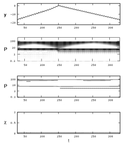
Figure 2: Analysis of the non-resonant 3-body interaction. The schematic interaction is presented in fig.  1 and the initial conditions are provided in tab. 1. The top panel gives the time series $y(t)$ of star #2. The sinusoidal line to the bottom right shows a projection of the orbital motion of star #2. The second panel contains the CWaT for this time series, followed by the ridge extraction in the third panel from above. The bottom panel shows the $\chi$ according to equation 5.

3.2 Irregular motion in a democratic resonant interaction

In a democratic resonance encounter the incoming star interacts closely with both components of the initial binary, until one of the stars eventually escapes. The initial conditions used for this example are presented in Tab. 2 and a schematic representation of the interaction is shown in fig.  3, and the analyse using CWaT is presented in fig.  4.

This interaction is considerably more complicated that the previous two examples. In fig. 3 and 4 we see how the incomer, star #3, is captured by the binary (consisting of star #1  and #2) at $t\simeq 400$ and interacts several times strongly with the other two stars before being ejected again at $t\simeq 1700$. The initial binary has a period $P\simeq 6.3$, but after $t\simeq 400$ the CWT becomes very irregular. The most irregular regime is noticeable in the analysis for $\chi$ in the bottom panel of fig. 4 at $t=[450,1700]$, with a peak near $t=[750,1000]$, where values of $\chi\ {\raise-2.15277pt\hbox{$\buildrel>\over{\sim}$}}\ 0.6$ are reached.

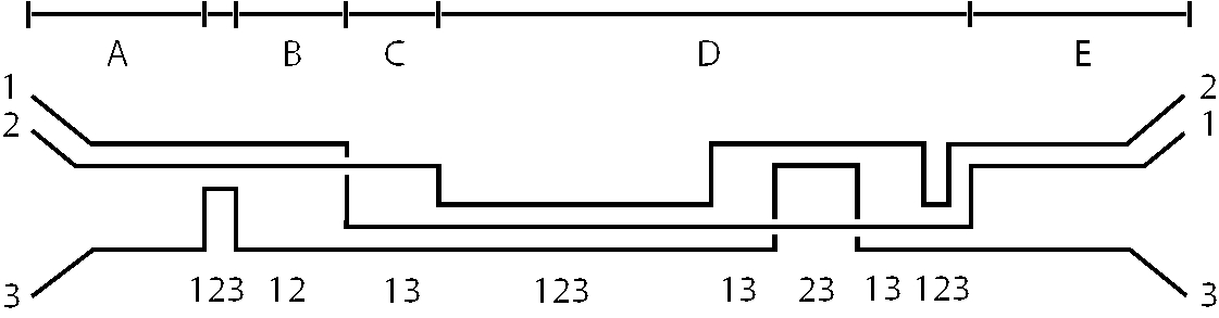
Figure 3: Schematic representation for the democratic resonant 3-body interaction. The analysis of this interaction is given in fig.  4.

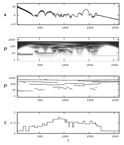
Figure 4: Analysis of the democratic resonant 3-body interaction from fig. 3. The analysis is based on the time-series $x(t)$ of star #1.

The strong democratic resonance interaction in this §  provides an excellent example to compare the CWaT method with Poincaré sections, which we will do in the subsequent §.

3.3 Poincaré section of a democratic resonant interaction

Poincaré sections have, like the CWaT diagnostic, the advantage that a qualitative impression of the irregularity in time series can be obtained instantaneously, id est; at run time. The main disadvantage of Poincaré sections is the required choice of a fundamental plane. This hinders analysis of complicated orbits in larger $N$-body systems, as there is no simple automated procedure to find a fundamental plane through which the Poincaré section can be taken. This is in particular a problem in systems with hierarchical substructure, such as the motion of moons around planets which again move around a star. The CWaT method does not suffer from this complication and, in addition, provides an unbiased indicator for the degree of irregularity. We here compare the CWaT method with Poincaré sections to demonstrate that global behaviour is reproduced in both methods.

Poincaré sections are computed using the velocity components of a star along a fundamental plane and record the moments a star passes through that plane. A stable binary in this representation gives a linear relation between the velocity components at each intersection. For the democratic resonant interaction of § 3.2 we use the velocity components of star #1  in the $v_{x}v_{z}$-plane at the moments $v_{y}$ becomes negative. The centre of mass of the 3-body system remains in the origin throughout the simulation. The results of this are presented in fig  5.

In fig  5 we indicate the five epochs by the letters ’A’ through ’E’. The same designation is used in fig. 3. The points is regions ’A’ and ’E’ are clustered together, indicating that the orbit of the star before (’A’) and after (’E’) is well behaved. During the resonant encounter (’B’, ’C’ and ’D’) each of these resonant epochs can be grouped with hindsight from the CWaT method. In fig. 5 we use different symbols to identify the various resonant epochs.

Figure 5: Poincaré section of the velocity components of the democratic resonant 3-body interaction shown in fig.  3 and further analysed in fig. 4. Here we show $v_{x}$ and $v_{z}$ for star #1 at each moment that $v_{y}$ becomes negative. The letters ‘A’, ‘B’, ‘C’ and ‘E’ correspond to the regions indicated in fig.  3. Scattered asterisks between region ‘B’ and ‘C’ belong to time interval indicated with ‘D’. The little squares indicate the short intermittent period between ‘A’ and ‘B’.

3.4 Irregular motion in a 100-body system

After having confirmed that the CWaT method enables a reliable detection of irregular orbits in small N-body systems it is time to focus on the larger systems. Here we will apply CWaT to self gravitating $N$-body systems with 100 particles. In particular we report here the result for several of such simulations. The initial realizations of the particle clusters ware generated as follows. We make a distinction between two basic models, model EqM and model S. Model EqM was constructed by distributing 100 objects of the same mass in a Plummer [45] Spherical density distribution. The velocity of all point masses are subsequently scaled such that the entire system is in virial equilibrium, and to $N$-body units [43]. We run the system for 100 $N$-body time units, which corresponds to about 35 dynamical time units.

In fig. 6 we present the evolution of several fundamental radii for simulation model EqM which contain 5%, 50% and 75% of the entire mass of the system. Although it is not our intention to discuss the dynamical evolution of this system it is worth mentioning that the core experiences a gravothermal runaway [46] at about $t\simeq 35$, noticeable as the deepest point reached by the lower solid curve (5% Lagrangian radius), whereas the outer parts of the cluster continues to expand, mainly due to binary heating.

Figure 6: Evolution of the radii which contains 5% (bottom thick solid curves), 50% (middle solid curve) and 75% (thin solid curve) of the mass for simulation model EqM (all masses are equal). For model S, with a Salpeter initial mass distribution for the individual particles, the same data is presented as the thick dotted curve (5% Lagrangian radius) and the two thin dotted curves representing the 50% and the 75% Lagrangian radii.

A further analysis of simulation EqM using CWaT, is presented in fig. 7. For each star we compute the CWT for the duration of the simulations. In fig. 7 we then show the fraction of stars ($f_{\rm EqM}$) which has a $\chi>0.1$ (top curve), 0.2, 0.4 and 0.6 (bottom curve). The various curves are rather smooth and flat. Some caution is well taken here, though, as near the edges (within the first and last $\sim 20$ time units) the CWaT becomes unreliable. The range between $t=20$ and $t=80$, where the method is accurate, we notice that the fraction of stars with any degree of chaoticity is roughly constant. It is interesting to note that $\ {\raise-2.15277pt\hbox{$\buildrel>\over{\sim}$}}\ 20$% of the stars have $\chi>0.6$ and that 30–40% of the stars have a $\chi<0.2$. In § 3.2, by the way, we demonstrated that a value of $\chi\ {\raise-2.15277pt\hbox{$\buildrel>\over{\sim}$}}\ 0.6$ is a strong indication that the underlying orbits change on a very short time scale. The core collapse around $t\simeq 35$ is not clearly noticeable. Core collapse has apparently no direct influence in the number of irregular orbits in the equal-mass $N$-body system.

Figure 7: The evolution of $f_{\rm EqM}$ for simulation model EqM, the fraction of stars with $\chi>0.1$, 0.2, 0.4 and 0.6 (from top to bottom).

We run a second simulation with the same number of particles, distributed initially using the same 3 dimensional density profile, in which we assign randomly masses to each of the stars from a power-law distribution. We opted for a [47] mass function which has the form of $N(m)\propto m^{-2.35}$. Here $N(m)$ is the number of stars formed per unit mass range. We apply this mass function over a range of two orders of magnitude, i.e, the most massive star is a hundred times more massive than the least massive stars. We call this model S.

We perform several simulations using this mass function but with new initial realizations of the system. The run-to-run variations can be quite large, mainly due to the small number of stars. A consistent trend, however, is evident.

The dotted curves in fig. 6 present the evolution of the fundamental radii containing 5%, 50% and 75% of the mass of simulation model S. The evolution of the structure of model S is quite different than for the simulation with equal masses (model EqM). In the former case core collapse occurs much earlier (at about $t=14$), which is consistent with simulations of [48]. However, model S also shows a second core collapse near $t\sim 63$. Noticeable is the much more dramatic expansion of the outer parts of the cluster, which is driven by the heating of the cluster core by close bound pairs which form during the core collapse (exempli gratia see [42, 49]).

Figure 8: The evolution of the ratio of $q\equiv f_{\rm S}/f_{\rm EqM}$. The solid and dotted curves are for two different realizations of the initial conditions of the $N$-body system with initial parameters according to model S. From top to bottom the curves are computed by adopting $\chi>0.1$ (top solid and dotted curves), 0.2, 0.4 and $\chi>0.6$ (bottom sold curve). To prevent clutter the latter value for $\chi$ is presented only for one of the simulations.

We compute the CWT for each star in model S, for which we show the results of two simulations. For a better comparison we present the ratio $q_{\rm S/EqM}\equiv f_{\rm S}/f_{\rm EqM}$ in fig. 8. Here $f_{\rm S}$ and $f_{\rm EqM}$ are computed for the same value of $\chi$, being either 0.1, 0.2, 0.4 or 0.6. Here the bottom curve represents the ratio in the number of stars for $\chi>0.6$, the two curves give $q_{\rm S/EqM}$ for $\chi>0.1$. The ratio $q_{S/EqM}<1$ for all values of $\chi>0.1$ and over the entire time span of the simulations.

The result of two simulations with a mass spectrum (solid and dotted curves, in fig. 8 show the same behaviour. The structure of the curves for $\chi>0.4$ and $\chi>0.6$ are also quite interesting. They continue to drop at a constant rate until model S reaches a second core collapse around $t=60$–70.

The comparison carried out here, though not the main objective of this paper, is quite interesting from an astrophysical perspective. As the multi-mass simulation systematically appears to have fewer stars on irregular orbits. This deficiency can be as small as $q=0.05$ during core collapse (or there about). We are currently extending this analysis to larger $N$-body systems on order to study core collapse in large $N$-body simulations.

4 Conclusions

We present a qualitative diagnostic to analyze irregular behaviour in particle based gravitational $N$-body simulations. The method, dubbed CWaT, is based on continuous wavelet transforms and provides a direct and instantaneous diagnostic for irregular behaviour.

In our analysis we demonstrate that CWaT is suitable for analyzing self gravitating $N$-body simulations, as it does not require a long time series for the analysis and it provides an instantaneous indicator for the degree of chaos, allowing a quantification of the number of irregular orbits at any moment in time in a large $N$-body simulation.

We applied CWaT successfully to analyse gravitational 3-body interactions. The results of the CWaT method for 3-body systems compares well with Poincaré sections. Here CWaT provides a qualification of the irregularity of the orbit, whereas for Poincaré sections such an analysis is technically much harder to perform.

Eventually we applied the CWaT method to several N-body systems with 100 particles in which all stars had the same mass, and another set of simulations in which a mass spectrum was adopted. The multi mass system systematically produced fewer stars on irregular orbits, compared to the equal mass system. In addition, we noticed that during a deep core collapse the number of irregular orbits dropped even further, whereas in the relatively low density inter-core collapse stages the number of irregular orbits tends to increases again.

Appendix: Initial conditions

The calculations for testing the method are performed with the kira integrator which is part of the starlab gravitational $N$-body environment [37] (see also http://www.manybody.org/manybody/starlab.html). The initial conditions used for the 3-body encounters used as examples in sections 3.1 and 3.2 are presented in the tables 1 and 2, respectively. The numbers in the tables are in standard $N$-body units [43]. Exact initial conditions for each of the three encounters studied is available via http://modesta.science.uva.nl. The CWaT source code is also upon request.

Table 1: Initial conditions of the non-resonant preserving 3-body interaction. All numbers are in N-body units The initial orbital parameters are: $m_{1}=m_{2}=m_{3}=0.5,a=1,e=0,b\simeq 1.34,v_{\infty}\simeq 1.24v_{c}$ where the critical velocity $v_{c}$ corresponds to a kinetic energy equal to the binding energy of the binary. [43].

star	mass	$x$-pos	$y$-pos	$z$-pos	$x$-vel	$y$-vel	$z$-vel
$1$	$0.5$	$-32.1139669$	$-19.6019186$	$2.424416360$	$-0.170641$	$0.431148$	$-0.0226399$
$2$	$0.5$	$-32.6179535$	$-20.465630$	$2.424416360$	$0.665287$	$-0.117690$	$-0.0226399$
$3$	$0.5$	$64.73192040$	$40.067549$	$-4.84883272$	$-0.494646$	$-0.313458$	$0.0452799$

Table 2: Initial conditions of the democratic resonant preservation 3-body interaction. The initial encounter parameters are $m_{1}=m_{2}=m_{3}=0.5,a=1,e=0,b\simeq 0.28,v_{\infty}\simeq 0.26v_{c}$.

star	mass	$x$-pos	$y$-pos	$z$-pos	$x$-vel	$y$-vel	$z$-vel
$1$	$0.5$	$11.02969588$	$-25.8888731$	$25.3364950$	$-0.498927$	$0.206499$	$-0.0524768$
$2$	$0.5$	$10.74875682$	$-26.8485987$	$25.3364950$	$0.453819$	$-0.0972697$	$-0.0524768$
$3$	$0.5$	$-21.7784527$	$52.7374718$	$-50.6729901$	$0.045107$	$-0.10923$	$0.104954$

References

- [1] P. Cipriani, M. Pettini, Strong Chaos in N-body problem and Microcanonical Thermodynamics of Collisionless Self Gravitating Systems, Ap&SS283 (2003) 347–368.
- [2] A. Einstein, Zur allgemeinen Relativitätstheorie, Sitzungsberichte der Königlich Preußischen Akademie der Wissenschaften (Berlin), Seite 778-786. (1915) 778–786.
- [3] A. Einstein, Zur allgemeinen Relativitätstheorie (Nachtrag), Sitzungsberichte der Königlich Preußischen Akademie der Wissenschaften (Berlin), Seite 799-801. (1915) 799–801.
- [4] A. Einstein, Die Grundlage der allgemeinen Relativitätstheorie, Annalen der Physik 49 (1916) 769–822.
- [5] G. Börner, E. Rudolph, Some Remarks on the General Relativistic 2-Body Problem, Mitteilungen der Astronomischen Gesellschaft Hamburg 43 (1978) 121.
- [6] F. Burnell, R. B. Mann, T. Ohta, Chaos in a Relativistic 3-Body Self-Gravitating System, Physical Review Letters 90 (13) (2003) 134101.
- [7] M. Delaunay, Note sur les Iné Lunaires às Pédues à l’action perturbatrice de Vé nus, MNRAS21 (1860) 60.
- [8] M. Delaunay, Note on the same subject, MNRAS20 (1860) 240.
- [9] Y. Kozai, Secular perturbations of asteroids with high inclination and eccentricity, AJ67 (1962) 591.
- [10] Y. Kozai, Secular perturbations of asteroids and comets, in: R. L. Duncombe (Ed.), IAU Symp. 81: Dynamics of the Solar System, 1979, pp. 231–236.
- [11] H. E. Kandrup, Chaos, Regularity, Noise in Self-Gravitating Systems, in: R. T. Jantzen, G. Mac Keiser, R. Ruffini (Eds.), Proceedings of the Seventh Marcel Grossman Meeting on recent developments in theoretical and experimental general relativity, gravitation, and relativistic field theories, 1996, p. 167.
- [12] R. H. Miller, How Important are the Equations of Motion in a Chaotic System?, Space Science Reviews 102 (2002) 115–120.
- [13] A. M. Lyapunov, Probleme general de la stabilite du mouvement, Vol. 9, Reed. Princiton University Press, 2000.
- [14] C. Froeschlé, E. Lega, R. Gonczi, Fast Lyapunov Indicators. Application to Asteroidal Motion, Celestial Mechanics and Dynamical Astronomy 67 (1997) 41–62.
- [15] R. Brasser, D. C. Heggie, S. Mikkola, One to One Resonance at High Inclination, Celestial Mechanics and Dynamical Astronomy 88 (2004) 123–152.
- [16] Z. Sándor, B. Érdi, A. Széll, B. Funk, The Relative Lyapunov Indicator: An Efficient Method of Chaos Detection, Celestial Mechanics and Dynamical Astronomy 90 (2004) 127–138.
- [17] C. Kalapotharakos, N. Voglis, G. Contopoulos, Chaos and secular evolution of triaxial N-body galactic models due to an imposed central mass, A&A428 (2004) 905–923.
- [18] C. Skokos, C. Antonopoulos, T. C. Bountis, M. N. Vrahatis, Detecting order and chaos in hamiltonian systems by the sali method, J. Phys. A37 (2004) 6269–6284.
- [19] D. D. Carpintero, L. A. Aguilar, Orbit classification in arbitrary 2D and 3D potentials, MNRAS298 (1998) 1–21.
- [20] Y. Papaphilippou, J. Laskar, Global dynamics of triaxial galactic models through frequency map analysis, A&A329 (1998) 451–481.
- [21] M. Valluri, D. Merritt, Regular and Chaotic Dynamics of Triaxial Stellar Systems, ApJ506 (1998) 686–711.
- [22] H. Poincaré, Les methodes nouvelles de la mecanique celeste, Gauthier-Villars, Paris 1.
- [23] G. A. Gottwald, I. Melbourne, A new test for chaos, nlin.CD/0208033.
- [24] P. Cipriani, M. T. Di Bari, Fast instability indicator in few dimensional dynamical systems (2002).
- [25] P. Goupillaud, A. Grossmann, J. Morlet, Cycle-Octave and related transforms in seismic signal analysis, Geoexploration 23 (1984) 85–102.
- [26] A. Grossmann, J. Morlet, Decomposition of hardy functions into square integrable wavelets of constant shape, SIMAT 15 (1984) 723–736.
- [27] S. Mallat, A wavelet tour of signal processing, Academic Press, 1998.
- [28] T. A. Michtchenko, D. Nesvorny, Wavelet analysis of the asteroidal resonant motion., A&A313 (1996) 674–678.
- [29] L. V. Vela-Arevalo, J. E. Marsden, Time–frequency analysis of the restricted three-body problem: transport and resonance transitions, Class. Quantum Grav. 21 (2004) 351–375.
- [30] S. Kirkpatrick, C. D. Gelatt, M. P. Vecchi, Optimization by Simulated Annealing, Science 220 (1983) 671–680.
- [31] V. Cerny, A thermodynamical approach to the travelling salesman problem: an efficient simulation algorithm, Journal of Optimization Theory and Applications 45 (1985) 41–51.
- [32] R. Carmona, W. Hwang, B. Torrésani, Practical Time-Frequency Analysis: continuous wavelet and Gabor transforms, with an implementation in S, Vol. 9 of Wavelet Analysis and its Applications, Academic Press, San Diego, 1998.
- [33] C. Chandre, S. Wiggins, T. Uzer, Time–frequency analysis of chaotic systems, Physica D: Nonlinear Phenomena 181 (2003) 171–196.
- [34] C. E. Delaunay, Cours elementaire d’astronomie, Paris, G. Masson [etc.] 1876. 6. ed., 1876.
- [35] P. T. Boyd, Binary-single star scattering: an investigation of a realistic chaotic scattering system, Ph.D. Thesis.
- [36] S. J. Aarseth, J. P. Anosova, V. V. Orlov, V. G. Szebehely, Global chaoticity in the Pythagorean three-body problem, Celestial Mechanics and Dynamical Astronomy 58 (1994) 1–16.
- [37] S. F. Portegies Zwart, S. L. W. McMillan, P. Hut, J. Makino, Star cluster ecology - IV. Dissection of an open star cluster: photometry, MNRAS321 (2001) 199–226.
- [38] S. F. Portegies Zwart, H. Baumgardt, P. Hut, J. Makino, S. L. W. McMillan, Formation of massive black holes through runaway collisions in dense young star clusters, Nature428 (2004) 724–726.
- [39] S. J. Aarseth, Multiple Time Scales, pub-AP, pub-AP:adr, 1985, Ch. Direct Methods for N-body Simulations, pp. 377–418.
- [40] J. Makino, S. J. Aarseth, On a Hermite integrator with Ahmad-Cohen scheme for gravitational many-body problems, PASJ44 (1992) 141–151.
- [41] P. Hut, J. N. Bahcall, Binary-single star scattering. I - Numerical experiments for equal masses, ApJ268 (1983) 319–341.
- [42] D. Heggie, P. Hut, The Gravitational Million-Body Problem: A Multidisciplinary Approach to Star Cluster Dynamics, The Gravitational Million-Body Problem: A Multidisciplinary Approach to Star Cluster Dynamics, by Douglas Heggie and Piet Hut. Cambridge University Press, 2003, 372 pp., 2003.
- [43] D. C. Heggie, R. D. Mathieu, Standardised Units and Time Scales, in The Use of Supercomputers in Stellar Dynamics, ed. P. Hut & S. L. W. McMillan (Berlin: Springer) 267 (1986) 233.
- [44] C. Chandre, T. Uzer, Instantaneous frequencies of a chaotic system, Pranama j. Phys 64 (2005) 371–380.
- [45] H. C. Plummer, On the problem of distribution in globular star clusters, MNRAS71 (1911) 460+.
- [46] D. Sugimoto, E. Bettwieser, Post-collapse evolution of globular clusters, MNRAS 204 (1983) 19P–22P.
- [47] E. E. Salpeter, The luminosity function and stellar evolution., ApJ121 (1955) 161.
- [48] S. F. Portegies Zwart, S. L. W. McMillan, Gravitational thermodynamics and black-hole mergers, Int, J, of Mod. Phys, A 15 (2000) 4871–4875.
- [49] S. A. Aarseth, Gravitational N-body simulations, Cambdridge University press, 2003, 2003.