Self-Similar Evolutionary Solutions of Self-Gravitating, Polytropic $\beta$-Viscous Disks

Abstract

Aims. We carry out the effect of $\beta$-prescription for viscosity which introduced by Duschel et al. 2000 & Hure, Richard & Zhan 2001, in a standard self-gravitating thin disks. We were predicted in a self-gravitating thin disk the $\beta$-model will have different dynamical behavior compare the well known $\alpha$-prescriptions.

Methods. We used self-similar methods for solving the integrated equations which govern the dynamical behavior of the thin disks.

Results. We present the results of self-similar solutions of the time evolution of axisymmetric, polytropic, self-gravitating viscous disks around a new born central object. We apply a $\beta$-viscosity prescription which has been derived from rotating shear flow experiments ($\nu=\beta r^{2}\Omega$). Using reduced equations in a slow accretion limit, we demonstrate inside-out self-similar solutions after core formation in the center. Some physical quantities for $\beta$-disks are determined numerically.We have compared our results with $\alpha$-disks under the same initial conditions. It has been found that the accretion rate onto the central object for $\beta$-disks more than $\alpha$-disks at least in the outer regions where $\beta$-disks are more efficient. Our results show that Toomre instability parameter is less than one everywhere on the $\beta$-disk which means that in such disks gravitational instabilities can be occurred, so the $\beta$-disk model can be a good candidate for the origin of planetary systems. Our results show that the $\beta$-disks will decouple in the outer part of the disk where the self-gravity plays an important role which is in agreement with Duschl predictions.

1 Introduction

Accretion disks are recognized as one of the objects that are found around many astrophysical objects, such as active galactic nuclei AGN, binary stars and young stellar objects. On the observational side, evidence for disks in young stellar objects gleaned both spectroscopically and through direct imaging is now quite compelling (Beckwith $\&$ Sargent 1993, Storm et al, 1993). Up to half of the solar type, pre-main sequence stars are surrounding by diks of gas and dust, many of these disks having masses similar to that expected for the early solar nebula (Chandler, C. J. 1998). The accretion disks around pre-main sequence stars are good candidates for the creation of planetary systems. The structure of such disks is a subject of great interest and has been studied both through self-similar solutions assuming unsteady state (Mineshige $\&$ Umemura 1997; Mineshige et al. 1997; Tsuribe 1999) and through direct numerical hydrodynamical simulations (Igumenshchev $\&$ Abramowicz 1999; Stone et al. 1999; Torkelsson et al. 2000). It is understood that the most crucial factors are self-gravity and viscosity which have great role on angular momentum transportation on the gas disk. Accretion takes place because of the action of some form of dissipation which releases the free energy of the shear flow as heat, and so allows the disk material to fall deeper into the potential well of the central object. In a simple picture ,Lynden-Bell and Pringle (1974) indicated that the dissipative processes must take the form of a stress which transport angular momentum outwards. It plays a significant role in many such systems, ranging from protostellar disks to active galactic nuclei (AGN). The self-gravity will modify the radial and vertical equations and so can treat the dynamical behavior of the accretion disks. In the standard thin accretion disk model, the effect of self-gravity is neglected, and only pressure supports the vertical structure. By contrast, the theory of self-gravitating accretion disks is less developed and in the traditional model of accretion disks, the self-gravity is ignored just for simplicity (e.g. Pringle 1981), although the self-gravity can describe the deviation from Keplerian rotation velocity in some AGN and flat infrared spectrum of some T Tauri stars. From the observational point of view, there are already some clues that the disk self-gravity can be important both in the context of proto-stellar disks and in the accretion disks around super massive black holes in the AGN. However, the detailed comparison with observations is limited by the lack of detailed models of self-gravitating disks and by an incomplete understanding of the basic physical processes involved.

The study of self-gravity in a most general case is difficult and because of these complexities, authors usually study the effects related to the self-gravity either in the vertical structure of the disk (e.g. Bardou et al. 1998) or in the radial direction (e.g. Bodo $\&$ Curir 1992). Disks in the AGN are thought to be relatively light in the sense that the ratio of $\frac{M_{d}}{M_{*}}$ is around a few percents (where $M$ and $M_{*}$ are the masses of the the disk and central star). Usually self-gravity plays its role at large distances from the central objects (Shlosman $\&$ Begelman 1987), and mainly in the direction perpendicular to the plane of the disk. But in the accretion disks around young stellar objects or pre-main-sequence stars, self-gravity can be important in all parts of the disk in both vertical and radial directions. Early numerical works of self-gravitating accretion disks began with N-body modelling (Cassen $\&$ Moosman 1981 ; Tomley, Cassen $\&$ Steinman-Cameron 1991). Shlosman $\&$ Begelman (1987) investigated the role of self-gravity in AGN. Recently, Ghanbari and Abbassi (2004) introduced a toy model which shows that at least in equilibrium of a thick accretion disk, self-gravity is an important effect.

One of the basic concepts of the theoretical descriptions of accretion disks and these dynamics, is the detailed knowledge underlying the physics of viscosity in the disks. Because of all detailed modeling of the structure and evolution of accretion disks depending on the viscosity and its dependence on the physical parameters, choosing the best viscosity model is quite important. There is a belief that, the molecular viscosity is inadequate to describe the observational evidence of some luminous accretion disks so some kinds of turbulence viscosity are required. Most investigators adopt so-called $\alpha$-model introduced by Shakura (1972) and Shakura $\&$ Sanyeav (1973) that gives the viscosity as the product of pressure scale height in the disk ($h$), the velocity of the sound ($c_{s}$) and a parameter $\alpha$ which contains all unknown physics. The models for the structure and evolution of accretion disks in close binary systems (e.g. dwarf novae and symbiotic stars) show that Shakura and Sunyeav’s parametrization with a constant $\alpha$ leads to results that reproduce the overall observed behavior of the disks quite well. And it has been recently recognized that accretion disks treated by a week magnetic field are subjected to MHD instabilities (Balbus $\&$ Hawly 1991), that can induce some kind of turbulence in the disk, thereby being able to transport angular momentum and to promote accretion processes. However in many astrophysically interesting cases, such as the outer part of proto-stellar disks, the ionization level is expected to be low, reducing significantly the effect of magnetic field in the dynamical behaviour of the disk. The realization that molecular transport of angular momentum is so inefficient led the theoreticians to look for another mechanism of transport of angular momentum in accretion disks. The alternative mechanism that would be a good candidate for transporting angular momentum in accretion disks is any kind of turbulence. Actually the $\alpha$-prescription is based on a kind of turbulence viscosity but it has not any physical base to drive the origin of turbulence in the model. On the other hand, laboratory experiments of Taylor-Couette systems seem to indicate that, although Coriolis force delays the onset of turbulence, the flow is ultimately unstable to turbulence for Reynolds numbers larger than a few thousands (e.g., see , Richard, Zahn, 1999 and Hure, Richard, Zahn 2001). Since in all kind of self-gravitating disks the Reynolds number is extremely high, it was thought that the hydrodynamical driven turbulent viscosity based on critical Reynolds number has probably significant role in the distribution of angular momentum in the accretion disks. The resulting turbulence would then transport angular momentum efficiently. Recently, Duschl, Stirittmatter and Biermann (2000) have proposed a generalized accretion disk viscosity prescription based on the hydrodynamically driven turbulence at the critical effective Reynolds number,$\beta$-model , which is applied for both self-gravitating and non self-gravitating disks and is shown to yield the standard $\alpha$-model in the case of the shock dissipation limited, non self-gravitating disks. They have shown that in the case of fully self-gravitating disks this model may explain the observed spectra of proto-planetary disks and yield a natural explanation for the radial motions from the observed metallicity gradients in the disk galaxy.

The basic equilibrium and dynamical structure of accretion disks are now well understood, as long as the standard model based on the $\alpha$-viscosity prescription (Shakura $\&$ Sunyeav 1973) is believed. Nevertheless, it is not easy to follow its dynamical evolution, mainly because the basic equations of the system are highly non-linear, specially when the system is self-gravitating (Paczynski 1978; Fukue $\&$ Sakamoto 1992). To follow the non-linear evolution of dynamically evolving systems, in general, the technique of the self-similarity is sometimes useful. Self-similar assumptions enable us to simplify the governing equations. Self-similar solutions have a wide range of applications in astrophysics. Several classes of self-similar solutions were known previously (Pringle 1974, Filipov 1984), but all of them considered the disk in a fixed, central potential. But a class of self-similar solution had been provided during last years that contained self-gravity (Mineshige $\&$ Umemura 1997). They had found a self-similar solution for a time evolution of isothermal, self-gravitating $\alpha$-viscous disk. This solution describes a homologous collapse of a disk via self-gravity and viscosity. They found that the disk structure and evolution are distinct in the inner and outer parts. The effect of self-gravity in the collapse of polytropic self-gravitating viscous disk has been investigated by Mineshige, Nakayama and Umemura (1997).

Following the Duschl et al. (2000) suggestion for $\beta$-prescription for viscosity, we apply this model for a thin self-gravitating disk around newborn stars. At first, it may seem that using other forms of viscosity is not an important issue, because just one should change the mathematical forms of the equations. But this simplified appearance did not force authors from such studies because of possible interesting results that one may obtain from other viscosity prescriptions. All these lead us to explore a self-gravitating disk using other viscosity prescriptions. However, all viscosity prescriptions are suffering from having phenomenological backgrounds rather than physically confirmed backgrounds. We think while we don’t have a clear picture of the turbulence in disks, all such prescriptions are standing on the same level as for their physical backgrounds. On the other hand, self-gravitation in a disk is a highly nonlinear process as a result of the complex behaviors of the various physical agents of the system, in which the turbulent viscosity and its prescriptions have a vital role. Thus, one may naturally ask what would happen if other forms of viscosity prescriptions in a self-gravitating disk is being used. When we searched in the literature, we found the $\beta$-prescription as only experimentally tested viscosity prescription. Indeed, there are few studies about $\beta$-prescription comparing the $\alpha$-model, clearly because of its newly proposed form. One may refer to many papers to see physical considerations and applications of the $\beta$-model: Mayer & Duschl (2005); Weigelt et al. (2004); Pott et al. (2004); Granato et al. (2004); Mathis, Palacios & Zahn (2004); Richard & Davis (2004). We expect to find different dynamical behaviors and we will show that in these disks the gravitational fragmentation can take place everywhere in the disks. So it will be a good description for the formation of a proto-planetary disk.

2 Formulation of Equations for Self-Similar Variables

Self-similar behavior provides a set of unsteady solutions to the self-gravitating fluid equations. On the other hand, many physical problems often attain self-similar limits for a wide range of initial conditions. Also self-similar properties allow us to investigate properties of the solutions in arbitrary detail, without any of the associated difficulties of numerical hydrodynamics.

2.1 The Basic Equations

In order to study the accretion processes of a thin disk under the effect of the self-gravity and viscosity, we consider axisymmetric polytropic disks using the cylindrical coordinates ($r,\phi,z$). We assume that the accretion disks are geometrically thin in the vertical direction and symmetric in the azimuthal direction. The model is described by the fundamental governing equations which are written as follow :

$$\\ \frac{\partial\rho}{\partial t}+\frac{1}{r^{2}}\frac{\partial}{\partial r}(r^{2}\rho v_{r})=0$$ (1)

$$\\ \frac{\partial v_{r}}{\partial t}+v_{r}\frac{\partial v_{r}}{\partial r}-\frac{v_{\phi}^{2}}{r}=-\frac{1}{\rho}\frac{\partial p}{\partial r}-\frac{\partial\Phi}{\partial r}$$ (2)

$$\\ \rho\frac{\partial(rv_{\phi})}{\partial t}+\rho v_{r}\frac{\partial(rv_{\phi})}{\partial r}=\frac{1}{r^{2}}\frac{\partial}{\partial r}(\nu\rho r^{4}\frac{\partial\Omega}{\partial r})$$ (3)

where $\rho$, $p$, $v_{r}$ and $v_{\phi}$ are density, pressure, radial and azimuthal components of velocity of the gas disk and also $\Phi$ is the gravitational potential of the gas disk inside of the radius r. We assume a polytropic relation between the gas pressure and density :

$$\\ P=K\rho^{\gamma}$$ (4)

with K and $\gamma$ being constants. The polytropic index $\gamma$ describes the adiabatic pressure-density relation. In subsequent analysis, we vary it and represent its effect on some physical quantities. The vertical extent of the disk at any radius is given by h, the half thickness of the disk:

$$\\ h=\frac{c_{s}}{(4\pi G\rho)^{\frac{1}{2}}}=\frac{c_{s}^{2}}{2\pi G\sigma}$$ (5)

where $c_{s}$ is the sound speed and $\sigma$ is the surface density.

The solution of these equations, give us the dynamical evolution of the disk which strongly depend on the viscosity model. So the study of dynamical behavior of the accretion disks is postponed to the more information about the viscosity.

2.2 Nondimensionalization

Before we actually begin solving equations (1)-(3), it is convenient to nondimensionalize the equations. The essence of self-similar model is the existence of only two dimensional parameters in the problem, viz., $K$ and the gravitational constant G. It is assumed, and this is born out by numerical calculations, that any additional parameters, such as the initial central density affects only transients, and theis memory is quickly lost, at least in the part of the flow in which the density greatly exceeds the initial central density. If that is the case, then only one dimensionless combination of radius r and time t can be found (Mineshige et al. 1997, Yahil 1983):

$$\\ \xi=K^{-\frac{1}{2}}G^{\frac{\gamma-1}{2}}r(t)^{\gamma-2}$$ (6)

This determines the dimensionless parameterizations of any similarity solution (Mineshige et al. 1997). Note that, we consider only $t>0$ for our work and the origin of time $(t=0)$ corresponds to the core formation epoch. Hence we have:

$$\frac{\partial}{\partial t}=\frac{\partial}{\partial t^{\prime}}+(\gamma-2)\frac{\xi}{t^{\prime}}\frac{\partial}{\partial\xi}$$ (7)

and

$$\frac{\partial}{\partial r}=K^{-\frac{1}{2}}G^{\frac{\gamma-1}{2}}(t^{\prime})^{\gamma-2}\frac{\partial}{\partial\xi}$$ (8)

for the transformation $(t,r)\rightarrow(t^{\prime}=t,\xi)$. Self-similarity allows us to reduce the self-gravitating fluid equations from partial differential equations into ordinary differential equations.

For changing the variables to dimensionless form, we used K and G; because we require that all of the time-dependent terms disappear in the self-similar forms of the equations. Other physical quantities (functions of t and r) are transformed into self-similar ones (functions of only $\xi$) as:

$$v_{r}(t,r)=K^{\frac{1}{2}}G^{\frac{1-\gamma}{2}}(t)^{1-\gamma}V_{r}(\xi),$$ (9)

$$v_{\phi}(t,r)=K^{\frac{1}{2}}G^{\frac{1-\gamma}{2}}(t)^{1-\gamma}V_{\phi}(\xi),$$ (10)

$$j(t,r)=KG^{1-\gamma}(t)^{3-2\gamma}J(\xi),$$ (11)

$$\sigma(t,r)=(2\pi)^{-1}K^{\frac{1}{2}}G^{-\frac{1+\gamma}{2}}(t)^{-\gamma}\Sigma(\xi),$$ (12)

$$\rho(t,r)=(4\pi\gamma)^{-\frac{1}{\gamma}}K^{\frac{1}{2}}G^{-1}(t)^{-2}\Sigma^{\frac{2}{\gamma}}(\xi),$$ (13)

$$p(t,r)=(4\pi\gamma)^{-1}KG^{-\gamma}(t)^{-2\gamma}\Sigma^{2}(\xi),$$ (14)

$$\nu(t,r)=KG^{1-\gamma}(t)^{3-2\gamma}\nu^{\prime}(\xi)$$ (15)

$$m(t,r)=K^{\frac{3}{2}}G^{\frac{1-3\gamma}{2}}(t)^{4-3\gamma}M(\xi).$$ (16)

where

$$J=\xi V_{\phi}\leavevmode\nobreak\ \leavevmode\nobreak\ \leavevmode\nobreak\ ,\leavevmode\nobreak\ \leavevmode\nobreak\ \leavevmode\nobreak\ \leavevmode\nobreak\ M=\frac{\xi\Sigma u}{3\gamma-4}.$$ (17)

with respect to another form for the continuity equation :

$$\frac{\partial m}{\partial t}+v_{r}\frac{\partial m}{\partial r}=0\leavevmode\nobreak\ \leavevmode\nobreak\ \leavevmode\nobreak\ \leavevmode\nobreak\ \leavevmode\nobreak\ \leavevmode\nobreak\ ,\leavevmode\nobreak\ \leavevmode\nobreak\ \leavevmode\nobreak\ \leavevmode\nobreak\ \leavevmode\nobreak\ m=2\pi\int_{0}^{r}\sigma rdr$$ (18)

thus, we have

$$\dot{M}=\frac{\xi\Sigma V_{r}}{3\gamma-4}$$ (19)

In order to solve the equations, we need to assign the kinematic coefficient of viscosity $\nu$. Although there are many uncertainties about the exact form of viscosity, as we mentioned in Introduction, we employ the $\beta$-prescription introduced by Duschl et al.:

$$\\ \nu^{\prime}=\beta\xi V_{\phi}$$ (20)

where $\nu^{\prime}$ is on a dimensionless form. We expect when the disk is non-self-gravitating, it leads to standard $\alpha$-prescriptions. With substituting this prescription into the above equations we can investigate the dynamical evolution of the disk.

2.3 Transformation of the basic Equations

Substituting the above transformations in equations (1)-(3), we can introduce a set of coupled ordinary differential equations. The basic equations are then transformed into the following forms:

$$\frac{1}{\xi}\frac{d}{d\xi}(\xi\Sigma u)=(3\gamma-4)\Sigma$$ (21)

$$u\frac{du}{d\xi}=-\frac{c^{2}}{\Sigma}\frac{d\Sigma}{d\xi}-\frac{M}{\xi^{2}}+\frac{J^{2}}{\xi^{3}}+(2\gamma-3)u+(2-\gamma)(\gamma-1)\xi$$ (22)

$$u\frac{dJ}{d\xi}=\frac{1}{\Sigma\xi}\frac{d}{d\xi}(\beta\xi^{3}\Sigma J\frac{d}{d\xi}(\frac{J}{\xi^{2}}))+(2\gamma-3)J$$ (23)

where $u$ is defined as,

$$u=V_{r}-(2-\gamma)\xi$$ (24)

and $c^{2}$ is a constant:

$$c^{2}=2(4\pi\gamma)^{\frac{1-\gamma}{\gamma}}\Sigma^{\frac{2\gamma-2}{\gamma}}$$ (25)

Now we have a set of complicated differential equations that must be solved under appropriate boundary conditions. Although a full numerical solutions to these equations would now be possible; it is more instructive to proceed by analyzing the model in some restrictive cases such as one on slow accretion limits.

3 Behavior of the Solutions

3.1 Slow Accretion Limit

We consider the fluid equations for a thin disk in the slow accretion approximation. The most substantive aspect of the slow accretion approximation consists of rotationally supported disks when the viscous timescale is much larger than the dynamical timescale. In addition, the pressure gradient force and the acceleration term in this approximation are ignored. The slow accretion approximation in disks has been used by Tsuribe (1999) and Minshige et al. (1997) and many others.

In the slow accretion limit ($|V_{r}|\ll 1\ll V_{\phi}$), and in the equation 2, the Euler equation, we have radial force-balance which means that only two terms on the right hand of the equation balance each other so we have:

$$\frac{J^{2}}{\xi^{3}}-\frac{M}{\xi^{2}}=0$$ (26)

hence we have:

$$J=(\xi M)^{\frac{1}{2}}=(\frac{\Sigma u}{3\gamma-4})^{\frac{1}{2}}\xi$$ (27)

We can make some simplifications in the equation of continuity in self-similar form, then it becomes:

$$\frac{dln\Sigma}{dln\xi}=-1-\frac{dlnu}{dln\xi}+(\frac{3\gamma-4}{u})\xi$$ (28)

Before driving other equations in a slow accretion limit, we introduce the distribution of the initial specific angular momentum, $j$, as (Tsuribe 1999):

$$j(r)=q{\frac{G}{c_{s}}}m(r)$$ (29)

where $j$ and $m$ are self-similar angular momentum and the total mass within the cylindrical radius r, respectively. The variable q is a dimensionless quantity has a constant value for the invicid equilibrium solutions (Mestel 1963; Toomre 1982) and variable value when the viscosity effect is included. Thus in dimensionless form,

$$J=qM$$ (30)

Now using Eqs.(27) and (30) we find that:

$$\Sigma^{\frac{1}{2}}=\frac{(3\gamma-4)^{\frac{1}{2}}}{qu^{\frac{1}{2}}}$$ (31)

With Eqs. (23),(24),(27) ,(28)and (31) we can finally find a simple differential equation for $V_{r}$:

$$\frac{dV_{r}}{d\xi}=\frac{q}{\beta}\frac{V_{r}[V_{r}\mp(2-\gamma)\xi]^{2}}{\xi[\pm 3V_{r}\mp(3\gamma-2)\xi]}+\frac{[3(2-\gamma)\pm 5(3\gamma-4)]V_{r}}{[\pm 3V_{r}\mp(3\gamma-2)\xi]}$$

$$+\frac{[(2-\gamma)(-18\gamma+22)\mp 2(3\gamma-4)^{2}]\xi}{[\pm 3V_{r}\mp(3\gamma-2)\xi]}$$ (32)

Now we can use the standard fourth-order Runge-Kutta scheme to integrate this ordinary differential equation. We can also use the asymptotic solutions of this equation near the origin and the outer part of the disk as a boundary condition.

3.2 Numerical Analysis

To solve equation (32) numerically, we need one boundary condition. We derived asymptotic solutions in the limits $\xi\rightarrow 0$ and $\xi\rightarrow\infty$ for $V_{r}$ where these asymptotic values can be used as boundary condition.

$$V_{r}=\frac{5\gamma-6}{6\gamma-7}\{\xi-\frac{q_{0}}{\beta}\frac{(\gamma-1)^{2}}{6\gamma-7}\xi^{2}\}\leavevmode\nobreak\ \leavevmode\nobreak\ \leavevmode\nobreak\ \leavevmode\nobreak\ \leavevmode\nobreak\ \leavevmode\nobreak\ \leavevmode\nobreak\ \xi\rightarrow 0$$ (33)

$$V_{r}=-\frac{\beta}{q_{0}}\frac{[(2-\gamma)(22-18\gamma)-2(3\gamma-4)^{2}]}{(2-\gamma)^{2}}\leavevmode\nobreak\ \leavevmode\nobreak\ \leavevmode\nobreak\ \leavevmode\nobreak\ \xi\rightarrow\infty$$ (34)

where $q_{0}$ is the asymptotic value of q in the outer radius. The equation (32) is integrated in the limits of the following equations (eqs. 33 and 34). It was found that only for some special values of the physical parameter such as $q,\gamma,\beta$ there exist physical solutions satisfied at both boundary conditions. By solving this equation we will have $V_{r}$ profile as a function of $\xi$ and other profiles ($V_{\phi},\Sigma\dot{M}...)$ can be obtained easily. In figures 1 and 2, we show radial and azimuthal velocity distributions for some $\gamma$ and $\beta$ values, respectively. Figures 3 and 4 indicate surface densities and mass accretion rates profiles for some $\gamma$ and $\beta$ values. Also we compare $\beta$ and $\alpha$ disks for $\gamma=1.1$ in all figures. The self-similar variables are functions of $\xi$. The behavior of the solutions predicted by the beta viscosity makes much more radial velocity (see Figure 1) compared to the $\alpha$-model (at least in the outer part of the disk where the self-gravity has an important role) and also for the azimuthal component of self-similar velocity, $\beta$-viscosity leads to faster velocities compared to the $\alpha$-model (see Figure 2). Therefore, the viscosity has more efficient role on the redistribution of angular momentum, and it leads to more radial flow and accretion rates.

It is predicted that the outer parts of a thin, viscous disk around QSOs, self-gravity has an important role. This effect is investigated by Toomre parameter (Toomre 1964), such that the local gravitational instability occurs where $Q<1$ and where $Q>1$ the disk is stable against the gravitational fragmentation. So it is useful to calculate Q values to compare gravitational stability in $\beta$ and $\alpha$ disks. The Toomre stability parameter for an epicyclic motion is:

$$Q=\frac{c_{s}k}{\pi G\sigma}=\frac{2J\sqrt{2}y}{\xi^{2}}K^{\frac{\gamma-1}{4}}(4\pi)^{\frac{1-\gamma}{2\gamma}}\gamma^{\frac{1}{2\gamma}}\Sigma^{\frac{-1}{\gamma}}$$ (35)

where

$$k=\Omega(4+2\frac{d\log\Omega}{d\log r})^{\frac{1}{2}}$$ (36)

is the epicyclic frequency and $\frac{dJ}{d\xi}=\frac{J}{\xi}y$. So if $\gamma=1$, we obtain $Q=\frac{2J\sqrt{2}y}{\Sigma\xi^{2}}$ (Tsuribe 1999).

In figure 5, we show the distribution of the Toomre Q value for some $\gamma$ and $\beta$ values. We also compare $\beta$ and $\alpha$ disks for $\gamma=1.1$. In figure 6, the angular momentum coefficient $q=\frac{J}{M}$ is plotted as a function of $\xi$ for some $\gamma$ values at $\beta=10^{-3}$. Also we see its behavior for $\beta$ and $\alpha$ disks.

4 Time scales

For estimating the effect of viscosity on the evolution of accretion disks we can compare the viscose time scale with dynamical time scale. The dynamical time scale $\tau_{dyn}$ is given by:

$$\tau_{dyn}=\frac{1}{\Omega}$$ (37)

where $\Omega$ in the non self-gravitating (NSG) and Keplerian self-gravitating (KSG) is given by the mass of the central accretor and by the radius. But in the fully self-gravitating disks, $\Omega$ is determined by solving Poisson’s equation. The time scale of viscose evolution $\tau_{visc}$ is given by:

$$\tau_{visc}=\frac{r^{2}}{\nu}$$ (38)

where in the standard non self-gravitating and geometrically thin accretion disks where $h<<r$ ( case $\alpha$-disks ), this leads to

$$\tau_{visc}^{non-SG}=(\frac{r}{h})^{2}\frac{\tau_{dyn}}{\alpha}$$ (39)

where in full self-gravitating (FSG) or KSG disks ( $\beta$-disks) is given by

$$\tau_{visc}^{FSG}=\tau_{visc}^{SG}=\tau_{visc}^{KSG}=\frac{\tau_{dyn}}{\beta}$$ (40)

So with $\alpha<1$ and $\beta<<1$ under all circumstances $\tau_{visc}>>\tau_{dyn}$. So the slow accretion limit will be confirmed. The best approximation for $\alpha$ parameter in the standard accretion model is less than one, $\alpha\sim 0.1$ but in the $\beta$ model which based on the critical Reynolds number beta is approximately $\beta\sim 10^{-2}-10^{-3}$. ($\frac{h}{r}$) in the outer part of accretion disks is too small, so in the outer part, of the disk where self-gravity of the disk dominates the beta viscous time scale is less than alpha viscous time scale. Therefore, the dynamical evolution of $\beta$-disks at least in the outer part is faster than the inner parts. Although, in the case of non-SG disks $\beta$-model can recover the standard $\alpha$-disks. So with $\beta$-model we can reconstruct a better picture in the equilibrium of galactic disks and protoplanetary disks. As we can see in the Fig.1, in comparison to alpha model, the radial flow in the beta disk is quite high which relevant to beta mechanism time scale. Because of the time scale of the beta disk is less, so it can evolve disks effectively and it can produce the large radial flow. In the case of galactic disks the inflow velocities in the $\beta$-model suggests values in the range $0.3-3kms^{-1}$ which is quite difficult to measure directly where $\alpha$-model suggest still lower values Duschl et al. (2000). Many authors have suggested the radial abundance gradients observed in our own and other disk galaxies maybe due to radial motion and diffusive mixing associated with the turbulence generated by eddy viscosity ( $\beta$-disks) (Lacey $\&$ Fall 1985, Sommer-Larsen $\&$ Yoshii 1990; Koppen 1994; Edmunds $\&$ Greenhow 1995). Such radial inflows are consistant with the $\beta$-model, but could be described with other physical processes such as the effect of magnetic field.

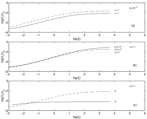
Figure 1: Radial self-similar velocity distributions as a function of self-similar variable $\xi$ for a) $\gamma=1.0,1.1$ at $\beta=10^{-3}$ b) $\beta=10^{-3},2\times 10^{-3},3\times 10^{-3}$ at $\gamma=1.1$ c) $\beta=10^{-3}$ and $\alpha=10^{-1}$ at $\gamma=1.1$.

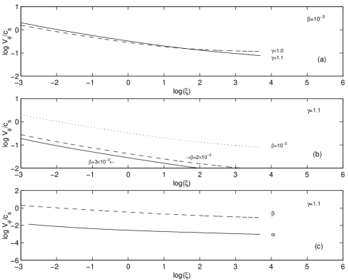
Figure 2: Azimuthal self-similar velocity distributions as a function of self-similar variable $\xi$, corresponding to a) $\gamma=1.0,1.1$ at $\beta=10^{-3}$ b) $\beta=10^{-3},2\times 10^{-3},3\times 10^{-3}$ at $\gamma=1.1$ c) $\beta=10^{-3}$ and $\alpha=10^{-1}$ at $\gamma=1.1$.

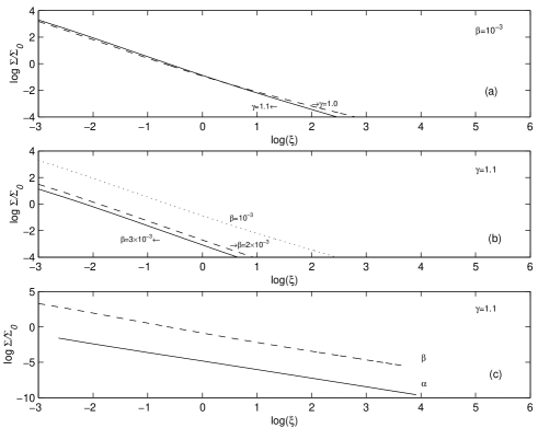
Figure 3: Self-similar Surface densities distributions as a function of self-similar variable $\xi$, corresponding to a) $\gamma=1.0,1.1$ at $\beta=10^{-3}$ b) $\beta=10^{-3},2\times 10^{-3},3\times 10^{-3}$ at $\gamma=1.1$ c) $\beta=10^{-3}$ and $\alpha=10^{-1}$ at $\gamma=1.1$

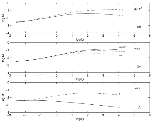
Figure 4: Self-similar mass accretion rates distributions as a function of self-similar variable $\xi$, corresponding to a) $\gamma=1.0,1.1$ at $\beta=10^{-3}$ b) $\beta=10^{-3},2\times 10^{-3},3\times 10^{-3}$ at $\gamma=1.1$ c) $\beta=10^{-3}$ and $\alpha=10^{-1}$ at $\gamma=1.1$

5 Concluding Remarks

The $\beta$-prescription based on the assumption that the effective Reynolds number of the turbulence dose not fall bellow the critical Reynolds number. In this parametrization the viscosity is proportional to the azimuthal velocity and the radius. This model yields physically consistent models of both Keplerian and fully self-gravitating accretion disks where in the case of thin disks with sufficiently small mass, recover the $\alpha$-disk solutions. Such $\beta$-disk models may be relevant to protoplanetary accretion disks (Duschl et al. (2000)). In the case of protoplanetary disks they yield spectra which are considerably flatter than those due to non-self-gravitating disks, in better agreement with observed spectra of these objects.

In this paper, we have considered the time-dependent evolution of self-gravitating disks with $\beta$-prescription by self-similar method for a thin, viscous disk. To do this, we started from dimensionless basic fluid equations. In order to dominate gravity and the centrifugal force, we consider the fluid equations for a thin disk in the slow accretion approximation. It has been found that evolution is described by solving a simple differential equation (32). We solved it numerically, beginning asymptotic solution of this equation near the origin as a boundary condition. Note should be taken that, we had the limitation to select parameter $\gamma$ for essence of differential equations and the fact that we seek just physical solutions.

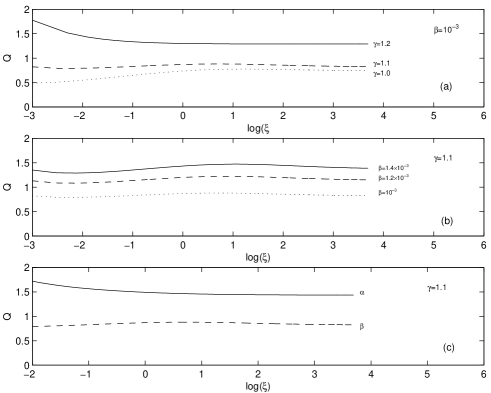
Figure 5: Distribution of the Toomre Q value as a function of self-similar variable $\xi$, corresponding to a) $\gamma=1.0,1.1$ at $\beta=10^{-3}$ b) $\beta=10^{-3},2\times 10^{-3},3\times 10^{-3}$ at $\gamma=1.1$ c) $\beta=10^{-3}$ and $\alpha=10^{-1}$ at $\gamma=1.1$.

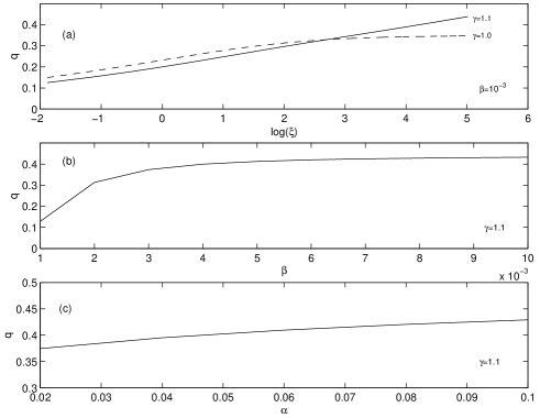
Figure 6: The angular momentum coefficient profile, q, as a function self-similar variable $\xi$ corresponding to a) $\gamma=1.0,1.1$ at $\beta=10^{-3}$. We see its behavior versus the dimensionless viscosity parameter for b) $\beta$ disks c) $\alpha$ disks at $\gamma=1.1$.

The presented method shows that an increase of $\beta$ value causes the azimuthal velocity to decrease but its general distribution function doesn’t vary throughout the disk. Also, azimuthal velocities in $\beta$-disks are far more than $\alpha$-disks (see Figure 2). So we expect the $\beta$-disks evolve in different ways with respect to the $\alpha$-disks.

According to Figure 4, $\beta$-disks have larger mass accretion rates than $\alpha$-disks. So, observably, we expect them to be brighter than $\alpha$-disks. Also, we note that with the increase of the $\beta$ value, $\dot{M}$ increases. Then mass flows increase onto the central object. This follows more radial velocity and less surface density (see Figures 1,3).

Comparing to $\alpha$-disks, q distribution ($q=\frac{J}{M}$) seems non-smoothly. The q values are very small in the innermost regions (see Figure 6). Whereas it is almost constant in the outer regions. It seems in the outer part of the disk where the beta viscosity is more efficient, the angular momentum is proportional to the disk’s mass inside the radius $r$. In order to study the effect of self-gravity of thin $\beta$-disks, we plot the Toomre parameter as a function of $\xi$. It is obvious that the gravitational instabilities in $\beta$-disks are more pronounced than $\alpha$-disks, $Q<1$. In Figure 5, Toomre parameter profile can reveal this subject. So it can be expected that the $\beta$-disk is a good model to describe planet formation around new-born stars. In a global overview, we showed that in the outer parts of the disk there is a difference between $\alpha$ and $\beta$ models. These results were predicated by Duschl et. al (2000).

Further, in order to study actual model and make a realistic picture for a thin self-gravitating disks, one must investigate energy exchange of the disk with its environment. In this case, one should find a mechanism for transferring the thermal energy from disk to outside environment; so we should add energy equation to our model. Both $\alpha$ and $\beta$ models are phenomenological prescriptions for disk viscosity. In an actual model of viscosity, it is possible to combine these two models and establish an exact description for different regions of the disk. Also in real accretion disks, there are many important processes other than viscosity that we have neglected. For example, non-axisymmetric waves which are also expected to transport angular momentum outward. Magnetic field and its influence are neglected and sometimes magnetic braking is another possibility for transporting angular momentum. However, these preliminary solutions can be the beginning of our understanding deployment from the physics governing the accretion disk.

References

- (1) albus, S., Hawly, J., 1991, APJ, 376, 214
- Bardou et al. (1998) Bardou, A., Heyvaerts, J., & Duschl, W. J. 1998, A&A, 337, 966
- Beckwith and Sargent (1993) Beckwith, S. V. W., & Sargent, A. I. 1993, ApJ, 402, 280
- Bodo and Curir (1992) Bodo, G., & Curir, A. 1992, A&A, 253, 318
- (5) Cassen, P., & Moosman A. 1981, Ikarus, 48, 353
- (6) Chandler, C. J. APS Conference series, Vol. 148, 1998
- (7) Duschl, W., Strittmatter, P. A., & Biermann P. L. 2000, A&A, 357, 1123
- Edmunds et al. (1995) Edmunds, M. G., & Greenhow, R. M. 1995, MNRAS, 272, 241
- (9) Filipov, L. G. 1984, Adv.Space Res., 3, 305
- (10) Fukue, J., & Sakamoto C. 1992, PASJ, 44, 553
- (11) Ghanbari, J., & Abbasi S. 2004, MNRAS, 350, 1437
- (12) Granato, G. L., De Zotti, G., Silva, L., Bressan, A., & Danese, L. 2004, ApJ, 600, 580
- (13) Huré, J. M., Richard, D., & Zahn, J. P. 2001, A&A, 367, 1087
- (14) Igumenshchev, I. V., & Abramowicz, M. A. 1999, MNRAS, 303, 309
- Koppen (1994) Koppen, J. 1994, A&A, 281, 26
- Lacey and Fall (1985) Lacey, C. G., & Fall, S. M. 1985, ApJ, 290, 154
- (17) Lynden-Bell, D., & Pringle, J. E. 1974, MNRAS, 168, 603
- (18) Mathis, S., Palacios, A., & Zahn, J. P. 2004, A&A, 425, 243
- (19) Mayer, M., & Duschl, W. J. 2005, MNRAS, 358, 614
- (20) Mestel, L. 1963, MNRAS, 126, 553
- (21) Mineshige, S., & Umemura, M. 1997, ApJ, 480, 167
- (22) Mineshige, S., Nakayama, K., & Umemura M. 1997, Publ.Astron.Soc, 49, 439
- (23) Paczynski, B., AcA, 1978, 28, 91
- (24) Pott, J. U., Hartwich, M., Eckart, A., Leon, S., Krips, M., & Straubmeier, C., 2004, A&A, 415, 27
- (25) Pringle, J. E. 1974, Ph.D.thesis,Univ.Cambridge
- (26) Richard, D., & Zahn, J. P., 1999, A&A, 347, 734
- (27) Richard, D., & Davis, S. S. 2004, A&A, 416, 825
- (28) Shakura, N. I. 1972, Astron.Zhur., 49, 921
- (29) Shakura, N. I., & Sunyaev, R. A. 1973, A&A, 24, 337
- (30) Shlosman, I., & Begelman, M. C. 1987, NATURE, 329, 29
- Sommer and Yoshii (1990) Sommer-Larsen, J., & Yoshii, Y. 1990, MNRAS, 243, 468
- Stone et al. (1999) Stone, J. M., Pringle, J. E., & Begelman, M. C. 1999, MNRAS, 310, 1002
- Storm et al. (1993) Storm, J. et al., 1993, RMXAA , 26, 105
- Tomley (1991) Tomley, L., Cassen, P., Steiman-Cameron, T. 1991, ApJ, 382, 530
- Toomre (1964) Toomre, A. 1964, ApJ, 139, 1217
- Toomre (1982) Toomre, A. 1982, ApJ, 259, 535
- Torkelsson et al. (2000) Torkelsson, U., Ogilvie, G. I., Brandenburg, A., Pringle, J. E., Nordlund, A., & Stein, R. F. 2000, MNRAS, 318, 47
- Tsuribe (1999) Tsuribe, T. 1999, ApJ, 527, 102
- Weigelt et al. (2004) Weigelt, G., Wittkowski, M., Balega, Y. Y., Beckert, T., Duschl, W. J., Hofmann, K. H., Men’shchikov, A. B., & Schertl, D. 2004, A&A, 425, 77
- Yahil (1983) Yahil, A. 1983, ApJ, 265, 1047