Supernovae, Lensed CMB and Dark Energy

Abstract

Supernova distance and primary CMB anisotropy measurements provide powerful probes of the dark energy evolution in a flat universe but degrade substantially once curvature is marginalized. We show that lensed CMB polarization power spectrum measurements, accessible to next generation ground based surveys such as SPTpol or QUIET, can remove the curvature degeneracy at a level sufficient for the SNAP and Planck surveys and allow a measurement of $\sigma(w_{p})=0.03$, $\sigma(w_{a})=0.3$ jointly with $\sigma(\Omega_{K})=0.0035$. This expectation assumes that the sum of neutrino masses is independently known to better than $0.1$ eV. This assumption is valid if the lightest neutrino is assumed to have negligible mass in a normal neutrino mass hierarchy and is potentially testable with upcoming direct laboratory measurements.

1. Introduction

Currently, observations of the expansion history of the universe are remarkably consistent with cosmic acceleration driven by a cosmological constant in a spatially flat universe. When testing this hypothesis, one typically looks for possible evidence of spatial curvature in the absence of dark energy evolution or evolution in the absence of spatial curvature. It is of course possible that spatial curvature and dark energy evolution conspire to mimic a cosmological constant in a flat universe. Nonetheless while the data remain consistent with the simpler hypothesis, this approach is justified.

More worrying is the possibility that as measurements improve, we find evidence for non-standard dark energy in a flat universe — a dark energy equation of state $w\neq-1$. Should we then believe that the universe is flat and dark energy varying in time, or that it has a small curvature and the dark energy is simply the cosmological constant? While the standard inflationary theory predicts that the curvature of our Hubble volume is below measurable limits ($\Omega_{K}\lesssim 10^{-4}$), models that allow a detectable spatial curvature do exist and are arguably on sounder footing than dynamical dark energy models.

Ideally of course, we would like to measure both $\Omega_{K}$ and $w(z)$ but this is difficult because of degeneracies. Moderately good constraints are obtained once type Ia supernova (SNe) data and cosmic microwave background (CMB) data are combined with high precision Hubble constant measurements (Hu 2005; Linder 2005), weak gravitational lensing (Knox 2006; Bernstein 2006), baryon oscillations (Knox et al. 2006; Ichikawa et al. 2006) or cluster abundances. However, these techniques are subject to a vast array of systematic uncertainties that have to be accounted for carefully. For example, weak gravitational lensing requires modeling of the fully nonlinear power on scales of 0.1-100 Mpc to the accuracy of a few percent (e.g., Huterer & Takada 2005).

Only two methods – SNe Ia and CMB – have proven so far to be both powerful and robust probes of cosmology. Here we show that the information required to break the degeneracy between curvature and dark energy to a level sufficient for future SNe missions such as SNAP (Aldering et al. 2004) lies within the reach of next generation ground-based CMB polarization power spectrum measurements. This information comes from weak gravitational lensing of the CMB in the linear regime at redshifts $z\sim 1-3$ (see Lewis & Challinor (2006) for a recent review). We employ a recently developed framework for CMB lensing power spectrum observables that includes the non-Gaussian nature of the lensing signal (Smith et al. 2006). This method is ideally suited for investigating the complementarity between different cosmological probes in a wide range of dark energy models.

2. Methodology

To describe the information content of the various cosmological probes, we model the observables and employ the usual Fisher approach. For SNe Ia, we model the magnitudes $m_{i}$ of the SNe as

$$m_{i}=5\log H_{0}d_{L}(z_{i})+\mathcal{M}+\epsilon_{i}\,,$$ (1)

where $i$ runs through the observed SNe. Here the luminosity distance is given by

$$d_{L}(z)=(1+z){1\over\sqrt{\Omega_{K}H_{0}^{2}}}\sinh\left(\sqrt{\Omega_{K}H_{0}^{2}}D\right)\,,$$ (2)

where $\Omega_{K}$ is the curvature in units of the critical energy density, $H_{0}$ is the Hubble constant, $D(z)=\int dz/H(z)$ is the comoving radial distance, $\mathcal{M}\equiv M-5\log H_{0}+25$ is a nuisance parameter involving the unknown absolute magnitude of the supernova $M$. The noise term $\epsilon_{i}$ represents both statistical errors and possible systematic errors that do not necessarily decrease with the number of observed supernovae.

Figure 1.— Top panel: redshift distribution of SNAP supernovae $n_{\rm SN}$ and weights of the lensing observables {$\Theta_{1},\Theta_{2}$} normalized to integrate to unity. Bottom panel: derivatives of the luminosity distance $d_{L}$ and relative luminosity distance $H_{0}d_{L}$ with respect to curvature $\Omega_{K}$ and the dark energy parameters $w_{0}$ and $w_{a}$. Here $\Omega_{\rm DE}$ is adjusted to keep the angular diameter distance to recombination fixed in each case.

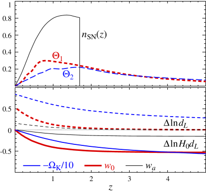
We assume a survey similar to the planned SNAP mission (Albert et al. 2005) with $2800$ SNe distributed in redshift out to $z=1.7$ given by Aldering et al. (2004) (middle curve of their Fig. 9, reproduced here in Fig. 1). We combine the SNAP dataset with 300 local supernovae uniformly distributed in the $z=0.03-0.08$ range.

Following Albert et al. (2005), we model the error as a sum of the statistical error and an irreducible, but unbiased, systematic error. The latter imposes a floor on the errors at a given redshift that is uncorrelated across broad redshift ranges. Given a binning of SNe into some arbitrary bins in $z$ denoted as $\Delta z_{I}$, we assume that

$$\sum_{i\in I,j\in J}{{\langle(m_{i}-\bar{m}_{i})(m_{j}-\bar{m}_{j})\rangle}\over N_{I}N_{J}}=\delta_{IJ}\left({\sigma_{m}^{2}\over N_{I}}+\sigma_{\rm sys}^{2}\right)\,,$$ (3)

where $N_{I}$ is the number of SNe in $\Delta z_{I}$. Following Tegmark et al. (1998), we can replace the sum over discrete SNe with an integral over the redshift distribution, $N_{I}=n_{\rm SN}(z)\Delta z_{I}$ and construct the Fisher matrix for a parameter set $p_{\mu}$ as

$$F_{\mu\nu}^{\rm SNAP}=\int dzn_{\rm SN}(z){1\over\sigma_{\epsilon}^{2}(z)}{\partial\bar{m}(z)\over\partial p_{\mu}}{\partial\bar{m}(z)\over\partial p_{\nu}}\,,$$ (4)

where

$$\sigma_{\epsilon}^{2}=\sigma_{m}^{2}+\sigma_{\rm sys}^{2}n_{\rm SN}(z)\Delta z\,.$$ (5)

For SNAP, we take $\sigma_{m}=0.15$ and $\sigma_{\rm sys}=0.02\,(1+z)/2.7$, $\Delta z=0.1$. When constructing the Fisher matrix in cosmological parameters we marginalize $\mathcal{M}$.

Figure 2.— Constraints on dark energy parameters $\Omega_{\rm DE}$, $w_{0}$ and $w_{a}$, shown for supernovae (SNAP) and unlensed CMB (Planck) separately: (a) constraints assuming a flat universe; (b) weakened constraints from curvature marginalization.

For the CMB, we use the information coming from recombination by constructing the Fisher matrix of the unlensed CMB out to multipole $\ell=2000$ in the usual way (Zaldarriaga et al. 1997). We assume the Planck survey with 80% usable sky and 3 usable channels for cosmology: FHWM $5.0^{\prime}$ with temperature noise $\Delta_{T}=51\mu$K^′ and polarization noise $\Delta_{P}=135\mu$K^′ ; $7.1^{\prime}$ with $\Delta_{T}=43\mu$K^′, $\Delta_{P}=78\mu$K^′; $9.2^{\prime}$ with $\Delta_{T}=51\mu$K^′, $\Delta_{P}=\infty$. We will call this Fisher matrix $F_{\mu\nu}^{\rm Planck}$.

For the additional information from lensing, we use the lensing observables framework (see Smith et al. 2006, for details). Constraints below so derived are an excellent match to those obtained through the full non-Gaussian band power covariance matrix. The two lensing observables $\Theta_{1}$ and $\Theta_{2}$ are determined from temperature/$E$-polarization and $B$-polarization respectively. They are associated with the amplitude of the convergence power spectrum in broad bands around $\ell_{1}\sim 100$ and $\ell_{2}\sim 500$. This amplitude in turn has a redshift sensitivity plotted in Fig. 1. Note that this sensitivity extends to $z\gg 1$ and is reason that CMB lensing has higher sensitivity to curvature than dark energy. The CMB lensing Fisher matrix is given by

$$F_{\mu\nu}^{\rm CMBlens}=\sum_{i=1,2}{\partial\Theta_{i}\over\partial p_{\mu}}{1\over\sigma^{2}_{\Theta_{i}}}{\partial\Theta_{i}\over\partial p_{\nu}}\,.$$ (6)

For the errors on the observables, we will assume a deep CMB survey that is comparable to the proposed SPTpol survey. Specifically we take a deep temperature survey on 4000 deg² and $\Delta_{T}=$ 11.5$\mu$K^′ and a deep polarization survey on 625 deg² with $\Delta_{P}=\sqrt{2}\Delta_{T}=4\mu$K^′. We take a FWHM beam of 1’. With these specifications combined with sensitivity to $\Theta_{1}$ from Planck, the two observables can be measured with an accuracy of $\sigma_{\Theta_{1}}=0.041$ and $\sigma_{\Theta_{2}}=0.032$. For reference, the latter represents a $\sim 3\%$ measurement of the overall power in lensing $B$-modes and dominates the overall constraints. Moreover the deep temperature survey provides little weight in the $\Theta_{1}$ constraint itself and would mainly serve as an internal cross check for foregrounds, systematics and other secondaries. Likewise, other planned surveys such as QUIET will have comparable precision in $\Theta_{2}$ with very different frequency bands.

Finally, we sum the Fisher matrices as usual

$$F_{\mu\nu}=F_{\mu\nu}^{\rm SNAP}+F_{\mu\nu}^{\rm Planck}+F_{\mu\nu}^{\rm CMBlens}$$ (7)

and approximate the joint parameter covariance matrix as $C_{\mu\nu}=({\bf F})^{-1}_{\mu\nu}$.

Figure 3.— 68% CL region in $w_{0}-w_{a}$ with and without CMB lensing (CMBlens) information. Filled ellipses: SNAP statistical errors. Open ellipses: SNAP systematic and statistical errors. Inner ellipse in each set: Planck+SNAP errors alone in a flat universe.

3. Forecasts with Curvature

It is well known that CMB information from recombination allows SNe to determine the dark energy equation of state parameters

$$w(a)=w_{0}+(1-a)w_{a}\,,$$ (8)

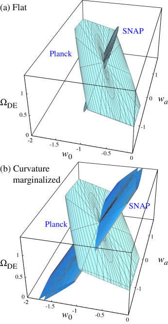
in a flat universe. In the 3-dimensional space {$\Omega_{\rm DE}$(=0.76), $w_{0}(=-1)$, $w_{a}(=0)$}, Planck CMB measurements limit the allowed region to a 2-dimensional surface or plane in the Fisher approximation (see Fig. 2). Values in parentheses represent those of the fiducial model. Here we have marginalized the baryon density $\Omega_{b}h^{2}(=0.022)$, cold dark matter density $\Omega_{c}h^{2}(=0.106)$, tilt $n_{s}(=0.958)$, initial amplitude of curvature fluctuations $\delta_{\zeta}(=4.52\times 10^{-5})$ at $k=0.05/{\rm Mpc}$, and reionization optical depth $\tau(=0.92)$.

SNAP supernovae measurements constrain a flat tube in this space that is nearly orthogonal to the Planck surface. Note that the pre-marginalization of any one of the three parameters before combining does not bring out this complementarity or the quality of the two surveys in confining the volume in the allowed dark energy space.

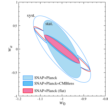
The marginalization of spatial curvature can be visualized as the superposition of independent shifts in the Planck plane and SNAP tube. Given that even the unlensed CMB has distance-independent, albeit weak, curvature information from both the ISW effect and the acoustic peaks (see Hu & White 1996, Fig. 11), the Planck plane only widens marginally (see Fig. 2). On the other hand the SNAP tube widens substantially. The net effect on the joint constraints in the $w_{0}-w_{a}$ plane marginalized over {$\Omega_{\rm DE}$, $\Omega_{K}$} is shown in Fig. 3. It represents a factor of 4.8 in the 68% CL area (Huterer & Turner 2001) as measured by $A_{w}=\sigma(w_{p})\sigma(w_{a})$. Here $w_{p}$ is the equation of state at the best constrained or pivot redshift and its errors are equal to those of $w_{0}$ at fixed $w_{a}$ (Hu & Jain 2004).

This degeneracy is also illustrated in Fig. 1 (bottom panel). Here the fractional deviations in the SNe observable $H_{0}d_{L}$ from the fiducial model are shown as parameter derivatives at a fixed distance to recombination. Without spatial curvature, $w_{0}$ and $w_{a}$ make distinguishable changes in the relative distance at $z<2$. With spatial curvature, the effects become largely degenerate.

The effect of spatial curvature on observables persists to high redshift $z\gg 1$ whereas that of the dark energy parameters flatten and depend only on $H_{0}$, the difference between relative and absolute distances. This degeneracy may therefore be broken either by high precision Hubble constant (Hu 2005; Linder 2005) or high-$z$ distance measurements (Knox 2006; Bernstein 2006).

Figure 4.— Improvement in the area statistic $A_{w}$ in the $w_{0}-w_{a}$ plane of as a function of the prior on the sum of the neutrino masses. The top line represents the SNAP+Planck constraint alone in a flat universe, the bottom represents the degradation once curvature is marginalized. CMB lensing can recover much of this information if the sum of the neutrino masses is known to $\sigma(m_{\nu})<0.1$eV.

CMB lensing supplies the latter kind of information. Around the fiducial model the sensitivity of the lensing observables to cosmological parameters used in Eqn. (6) is

$$\Delta\Theta_{1} \approx -1.01\Omega_{\rm DE}-0.399\Delta w_{0}-0.146\Delta w_{a}-5.17\Delta\Omega_{K}$$

$$+12.3\Delta\Omega_{c}h^{2}+2\Delta\ln\delta_{\zeta}-0.33{\Delta m_{\nu}\over 1{\rm eV}}\,,$$

$$\Delta\Theta_{2} \approx -1.27\Omega_{\rm DE}-0.446\Delta w_{0}-0.154\Delta w_{a}-5.30\Delta\Omega_{K}$$ (9)

$$+18.8\Delta\Omega_{c}h^{2}+2.09\Delta\ln\delta_{\zeta}-0.45{\Delta m_{\nu}\over 1{\rm eV}}\,.$$

This lensing sensitivity depends both on parameters that control distances and the matter power spectrum at the redshift range shown in Fig. 1. We have here used the fact that other parameters in the latter class such as $n_{s}$ are sufficiently well determined by Planck. The sum of the neutrino masses $m_{\nu}$ is however not well determined and changes both the shape and growth rate of the matter power spectrum. The distance parameters also change the growth rate and the curvature sensitivity is in fact enhanced by this effect.

First let us consider the impact of CMB lensing constraints assuming that the sum of the neutrino masses $m_{\nu}(=0.06$eV) is fixed. This is a good assumption if the lightest neutrino has a mass $<0.01$eV and a normal mass hierarchy due to the measurement of the solar and atmospheric neutrino mass squared differences. The same assumption in an inverted hierarchy would also be sufficient in that it only adds a second discrete possibility.

In this fixed neutrino case, the addition of the lensing constraint nearly fully restores the ability of SNAP and Planck to measure the dark energy (see Fig. 3). It allows a measurement to $\sigma(w_{a})=0.30$ and $A_{w}^{-1}=137$. This restoration of sensitivity occurs even if SNAP is limited by only statistical errors such that $\sigma(w_{a})=0.19$ and $A_{w}^{-1}=241$.

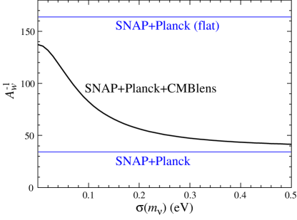
Figure 4 shows how $A_{w}^{-1}$ depends on prior knowledge of the sum of the neutrino masses in the case that the lightest neutrino does not have negligible mass. In this case all three neutrinos could have degenerate masses. External constraints on the sum of neutrino masses begin to help at the $0.2$eV level and would be fully sufficient at a few $10^{-2}$eV. For example the KATRIN experiment is expected to reach $\sigma(m_{\nu_{e}}^{2})=(0.16{\rm eV})^{2}$ from tritium $\beta$ decay (Aalseth et al. 2004). Such a measurement would test the degenerate mass scenario.

As an aside it is interesting to note that even with spatial curvature and dark energy the combination of data sets would allow a measurement of $\sigma(m_{\nu})=0.24$ eV. With curvature fixed, $\sigma(m_{\nu})=0.14$ eV. Hubble constant measurements with $1-7\%$ precision would provide neutrino measurements that interpolate between these two limits by fixing the spatial curvature.

4. Discussion

Constraints on the temporal evolution of dark energy benefit particularly strongly from the addition of CMB lensing information to that of SNe and the primary CMB at recombination. The three methods probe very different epochs: SNe are sensitive to distances at $z\lesssim 1$, the primary CMB to $z\sim 1089$ whereas CMB lensing probes $1\lesssim z\lesssim 3$. Given that spatial curvature affects distances and growth out to high redshift, CMB lensing is ideally suited to breaking the degeneracy between curvature and the dark energy. It has the additional advantage of being nearly entirely in the linear regime and a lensing test of curvature where the source distance can be considered fixed.

Furthermore, this degeneracy breaking requires only already planned ground-based CMB polarization power spectrum measurements. We have demonstrated that even if the SNAP and Planck surveys are limited only by statistical errors, a ground based survey like SPTpol will be sufficient to extract the full information: $\sigma(w_{p})=0.02$, $\sigma(w_{a})=0.2$ and $\sigma(\Omega_{K})=0.0034$; with some accounting for SNAP systematic errors these degrade to $0.025$, $0.3$, and $0.0035$.

There are two critical assumptions that make this possible. Firstly that the ground based CMB survey will be able to remove foregrounds and systematics at a level sufficient to enable few percent level measurements of the lensing $B$-mode polarization power. Secondly, we assume that the neutrino masses are fixed by oscillation measurements and a theoretical assumption about the neutrino mass hierarchy. This assumption will be tested by next generation laboratory experiments. In the more general context, the sum of the neutrino masses must be externally determined to $0.1$eV or better.

The lensing observables approach we have taken here can be easily extended to consider different combinations of probes or alternate explanations of the accelerated expansion. Furthermore we have only considered the simplest description of the time-dependent dark energy density, in terms of parameters $w_{0}$ and $w_{a}$. More ambitious descriptions of the dark energy sector or more exotic theoretical models with high redshift deviations may be even further assisted by CMB lensing.

References

- Aalseth et al. (2004) Aalseth, C., et al. 2004, APS Multidivisional Neutrino Study
- Albert et al. (2005) Albert, J., et al. 2005, DETF White Paper, astro-ph/0507458
- Aldering et al. (2004) Aldering, G., et al. 2004, astro-ph/0405232
- Bernstein (2006) Bernstein, G. 2006, The Astrophysical Journal, 637, 598
- Hu (2005) Hu, W. 2005, ASPC, 339, 215
- Hu & Jain (2004) Hu, W., & Jain, B. 2004, Phys. Rev. D, 70, 043009
- Hu & White (1996) Hu, W., & White, M. 1996, ApJ, 471, 30
- Huterer & Takada (2005) Huterer, D., & Takada, M. 2005, Astroparticle Physics, 23, 369
- Huterer & Turner (2001) Huterer, D., & Turner, M. S. 2001, Physical Review D, 64, 123527
- Ichikawa et al. (2006) Ichikawa, K., Kawasaki, M., Sekiguchi, T., & Takahashi, T. 2006, astro-ph/0605481
- Knox (2006) Knox, L. 2006, Physical Review D, 73, 023503
- Knox et al. (2006) Knox, L., Song, Y.-S., & Zhan, H. 2006, astro-ph/0605536
- Lewis & Challinor (2006) Lewis, A., & Challinor, A. 2006, Physics Reports, 429, 1
- Linder (2005) Linder, E. V. 2005, Astroparticle Physics, 24, 391
- Smith et al. (2006) Smith, K. M., Hu, W., & Kaplinghat, M. 2006, Physical Review D, submitted, astro-ph/0607315
- Tegmark et al. (1998) Tegmark, M., Eisenstein, D. J., Hu, W., & Kron, R. 1998, IAS preprint, astro-ph/9805117
- Zaldarriaga et al. (1997) Zaldarriaga, M., Spergel, D. N., & Seljak, U. 1997, ApJ, 488, 1