Cosmological Information from Lensed CMB Power Spectra

Abstract

Gravitational lensing distorts the cosmic microwave background (CMB) temperature and polarization fields and encodes valuable information on distances and growth rates at intermediate redshifts into the lensed power spectra. The non-Gaussian bandpower covariance induced by the lenses is negligible to $l=2000$ for all but the $B$ polarization field where it increases the net variance by up to a factor of 10 and favors an observing strategy with 3 times more area than if it were Gaussian. To quantify the cosmological information, we introduce two lensing observables, characterizing nearly all of the information, which simplify the study of non-Gaussian impact, parameter degeneracies, dark energy models, and complementarity with other cosmological probes. Information on the intermediate redshift parameters rapidly becomes limited by constraints on the cold dark matter density and initial amplitude of fluctuations as observations improve. Extraction of this information requires deep polarization measurements on only 5-10% of the sky, and can improve Planck lensing constraints by a factor of $\sim 2-3$ on any one of the parameters {$w_{0},w_{a},\Omega_{K},\sum m_{\nu}$} with the others fixed. Sensitivity to the curvature and neutrino mass are the highest due to the high redshift weight of CMB lensing but degeneracies between the parameters must be broken externally.

I Introduction

Primary cosmic microwave background (CMB) anisotropy from recombination has proven itself to be a veritable gold mine of cosmological information. One of the most important secondary signals that should be detected by upcoming cosmic microwave background experiments is the distortion to the temperature and polarization fields due to gravitational lensing by the large-scale structure of the universe (see Challinor and Lewis (2005) for a recent review). Lensing distortions add cosmological information on parameters such as curvature, neutrino masses and dark energy that change the expansion and growth rate at intermediate redshifts ($z\lesssim 5$).

This distortion in real space couples power in harmonic space and hence introduces non-Gaussianity into the CMB temperature and polarization fields. Beyond power spectra, this non-Gaussianity is a source of information in that it allows direct reconstruction of the convergence field Bernardeau (1998); Zaldarriaga and Seljak (1999); Hu (2001a); Hu and Okamoto (2002); Hirata and Seljak (2003). On the other hand, for purposes of extracting cosmological information from lensed power spectra as considered here, this non-Gaussianity is largely an impediment as it makes power spectrum estimates covary across a wide range of multipoles.

The purpose of this paper is twofold. First, we calculate the full non-Gaussian covariance between all combinations of temperature and polarization bandpowers in the lensed CMB. This extends previous work in which the temperature Hu (2001b); Cooray (2002) and $B$-mode polarization covariance Smith et al. (2004) were calculated separately. Second, we present a general framework for studying the extra information on cosmological parameters that lensed CMB spectra supply, with particular attention to the impact of non-Gaussianity.

Previous works have noted that the lensed CMB signal may be used to study the dark energy Hu (2002); Kaplinghat (2003); Acquaviva and Baccigalupi (2005) and neutrino mass Kaplinghat et al. (2003a). These studies did not compute the non-Gaussian covariance but assumed either that the information is encoded in the unlensed primary CMB and a reconstruction of the lenses or by approximating the non-Gaussian covariances with a degradation factor from Smith et al. (2004). Our results lend support to these analyses. We also study the sensitivity of lensing to curvature and find that future CMB measurements can provide interesting constraints on it.

This paper is organized as follows. In §II, we compute non-Gaussian contributions to the covariance between all lensed CMB temperature and polarization bandpowers. We then describe in §III how this non-Gaussian covariance propagates into Fisher matrix parameter forecasts and present formal bounds on its impact. In §IV, we define two parameter independent observables which contain essentially all information from the lensed CMB and discuss their relationship to distance and growth as well as their degeneracy with parameters that control the matter power spectrum. Armed with this general framework, we show how constraints on these observables can be interpreted in the context of common parameterizations of the dark energy and dark matter in §V. Finally in §VI we show how future CMB surveys can be optimized for sensitivity to the lensing observables. We conclude in §VII and briefly address the issues of goodness-of-fit in Appendix A and scaling with the fiducial cosmology in Appendix B.

II Lensed power spectrum covariance

In this section, we compute the non-Gaussian covariance between all CMB temperature and polarization bandpowers to lowest order in the lensing power spectrum $C_{l}^{\phi\phi}$. The results (Eqs. (II), (18), and (II)) will be foundational in subsequent sections, as they will permit the effects of non-Gaussianity to incorporated into parameter forecasts. However, the details of the calculation will not be needed, so the reader may wish to skip this section on a first reading.

First, we recall some preliminaries concerning lensed CMB fields. We work in the flat sky approximation; we will see (§III.2) that non-Gaussian covariance only becomes important when combining bandpowers over a wide range of $l$, so that all-sky corrections from the discrete nature of $l$ should be negligible. The lensed CMB temperature $T({\bf x})$ and unlensed temperature ${\widetilde{T}}({\bf x})$ are related by

$$T({\bf x})={\widetilde{T}}({\bf x}+\nabla\phi({\bf x}))\,.$$ (1)

The projected potential $\phi$ is given by the line-of-sight integral:

$$\phi(\widehat{\bf n})=2\int dD\frac{D_{A}(D_{s}-D)}{D_{A}(D)D_{A}(D_{s})}\Phi(D\widehat{\bf n},D)\,,$$ (2)

where $D=\int dz/H$ is the comoving distance along the line of sight, $D_{s}$ denotes the comoving distance to the surface of last scattering, and

$$D_{A}(D)={1\over\sqrt{\Omega_{K}H_{0}^{2}}}\sinh\left(\sqrt{\Omega_{K}H_{0}^{2}}D\right)$$ (3)

is the comoving angular diameter distance.

Polarization fields are lensed in the same way; the lensed Stokes parameters $Q({\bf x})$, $U({\bf x})$ and unlensed versions ${\widetilde{Q}}({\bf x})$, ${\widetilde{U}}({\bf x})$ are related by

$$Q({\bf x}) = {\widetilde{Q}}({\bf x}+\nabla\phi({\bf x}))\,,$$

$$U({\bf x}) = {\widetilde{U}}({\bf x}+\nabla\phi({\bf x}))\,.$$ (4)

The Fourier versions of Eqs. (1), (4) are Hu (2000):

$$T({\bf l}) = {\widetilde{T}}({\bf l})+\int\frac{d^{2}{\bf l}^{\prime}}{(2\pi)^{2}}W_{T}({\bf l},{\bf l}^{\prime}){\widetilde{T}}({\bf l}^{\prime})\phi({\bf l}-{\bf l}^{\prime})+{\mathcal{O}}(\phi^{2})\,,$$

$$E({\bf l}) = {\widetilde{E}}({\bf l})+\int\frac{d^{2}{\bf l}^{\prime}}{(2\pi)^{2}}W_{E}({\bf l},{\bf l}^{\prime}){\widetilde{E}}({\bf l}^{\prime})\phi({\bf l}-{\bf l}^{\prime})+{\mathcal{O}}(\phi^{2})\,,$$

$$B({\bf l}) = \int\frac{d^{2}{\bf l}^{\prime}}{(2\pi)^{2}}W_{B}({\bf l},{\bf l}^{\prime}){\widetilde{E}}({\bf l}^{\prime})\phi({\bf l}-{\bf l}^{\prime})+{\mathcal{O}}(\phi^{2})\,,$$ (5)

where the kernels are defined by

$$W_{T}({\bf l},{\bf l}^{\prime}) = -[{\bf l}^{\prime}\cdot({\bf l}-{\bf l}^{\prime})]\,,$$

$$W_{E}({\bf l},{\bf l}^{\prime}) = -[{\bf l}^{\prime}\cdot({\bf l}-{\bf l}^{\prime})]\cos 2(\varphi_{{\bf l}}-\varphi_{{\bf l}^{\prime}})\,,$$

$$W_{B}({\bf l},{\bf l}^{\prime}) = [{\bf l}^{\prime}\cdot({\bf l}-{\bf l}^{\prime})]\sin 2(\varphi_{{\bf l}}-\varphi_{{\bf l}^{\prime}})\,,$$ (6)

and the $E$ and $B$ fields are related to the Stokes parameters as

$$[E({\bf l})\pm iB({\bf l})]=[Q({\bf l})\pm iU({\bf l})]\exp(\mp 2i\varphi_{{\bf l}})\,.$$ (7)

Here $\varphi_{{\bf l}}$ is the angle between ${\bf l}$ and $\hat{\bf x}$ axis. We have assumed that the unlensed ${\widetilde{B}}=0$ such that the observed $B$ field is generated from ${\widetilde{E}}$ by lensing alone Zaldarriaga and Seljak (1998).

We define ideal, noise-free bandpower estimators by

$${\widehat{\Delta}}_{i}^{XY}=\frac{1}{A\alpha_{i}}\int_{{\bf l}\in i}d^{2}{\bf l}\,\left(\frac{l^{2}}{2\pi}\right)X^{*}({\bf l})Y({\bf l})\,,$$ (8)

where $XY\in\{TT,EE,TE,BB\}$, $A$ is the survey area in steradians, and

$$\alpha_{i}=\int_{{\bf l}\in i}d^{2}{\bf l}$$ (9)

is the $l$-space area of band $i$. We define power spectra as usual

$$\langle X^{*}({\bf l})Y({\bf l}^{\prime})\rangle = (2\pi)^{2}\delta^{2}({\bf l}-{\bf l^{\prime}})C_{{\bf l}}^{XY}$$ (10)

$$\approx A{\delta_{{\bf l},{\bf l^{\prime}}}}C_{{\bf l}}^{XY}\,,$$

such that

$$\Delta_{i}^{XY}\stackrel{{\scriptstyle\rm def}}{{=}}\langle{\widehat{\Delta}}_{i}^{XY}\rangle=\frac{1}{\alpha_{i}}\int_{{\bf l}\in i}d^{2}{\bf l}\,\left(\frac{l^{2}}{2\pi}\right)C_{{\bf l}}^{XY}\,.$$ (11)

(As a technical point, when propagating $C^{\phi\phi}_{l}$ to lensed power spectra, we use the all-sky correlation function approach of Challinor and Lewis (2005), for consistency with CAMB.)

Now let us consider the covariance of these estimators in non-overlapping $l$ bands. We split the bandpower covariance into Gaussian and non-Gaussian pieces:

$$C^{IJ} \stackrel{{\scriptstyle\rm def}}{{=}} \langle{\widehat{\Delta}}_{i}^{XY}{\widehat{\Delta}}_{j}^{ZW}\rangle-\Delta_{i}^{XY}\Delta_{j}^{ZW}$$ (12)

$$= {\mathcal{G}}_{ij}^{XY,ZW}+{\mathcal{N}}_{ij}^{XY,ZW}\,.$$

Here and below we will use the short hand notation $I$ to denote a unique bandpower specified by the $l$-band $i$ and the power spectrum $XY$. The Gaussian piece is given by:

$${\mathcal{G}}_{ij}^{XY,ZW} = \delta_{ij}\frac{(2\pi)^{2}}{A\alpha_{i}^{2}}\int_{{\bf l}\in i}d^{2}{\bf l}\,\left(\frac{l^{2}}{2\pi}\right)^{2}$$

$$\qquad\qquad\times(C_{{\bf l}}^{XZ}C_{{\bf l}}^{YW}+C_{{\bf l}}^{XW}C_{{\bf l}}^{YZ})\,,$$

where the power spectra which appear are lensed. In the presence of instrumental noise, the power spectra in this formula are replaced as

$$C_{{\bf l}}^{XY} \rightarrow C_{{\bf l}}^{XY}+N_{{\bf l}}^{XY}\,,$$ (14)

where the noise power spectra for white detector noise with a Gaussian beam are given by

$$N_{{\bf l}}^{XX}=\left({\Delta_{X}\over T_{\rm CMB}}\right)^{2}e^{l(l+1)\theta_{\rm FWHM}^{2}/8\ln 2}\,,$$ (15)

for $XX\in TT,EE,BB$ and vanishing for other spectra. We will also take $\Delta_{E}=\Delta_{B}=\Delta_{P}$.

In (Smith et al., 2004), we computed the non-Gaussian piece ${\mathcal{N}}_{ij}^{XY,ZW}$ for the case of two $BB$ bandpowers:

$${\mathcal{N}}_{ij}^{BB,BB} = \frac{2}{A\alpha_{i}\alpha_{j}}\int_{{\bf l}_{i}\in i}d^{2}{\bf l}_{i}\int_{{\bf l}_{j}\in j}d^{2}{\bf l}_{j}\int\frac{d^{2}{\bf l}}{(2\pi)^{2}}$$

$$\qquad\times\frac{l_{i}^{2}l_{j}^{2}}{(2\pi)^{2}}(a_{{\bf l}_{i}{\bf l}_{j}}^{{\bf l}}+b_{{\bf l}_{i}{\bf l}_{j}}^{{\bf l}}+c_{{\bf l}_{i}{\bf l}_{j}}^{{\bf l}})+{\mathcal{O}}(C_{l}^{\phi\phi})^{3}\,,$$

where

$$a^{{\bf l}}_{{\bf l}_{i}{\bf l}_{j}} = W^{2}_{B}({\bf l}_{i},{\bf l}_{i}-{\bf l})W_{B}^{2}({\bf l}_{j},{\bf l}_{j}-{\bf l}){\widetilde{C}}^{EE}_{{\bf l}_{i}-{\bf l}}{\widetilde{C}}^{EE}_{{\bf l}_{j}-{\bf l}}\big{(}C^{\phi\phi}_{{\bf l}}\big{)}^{2}\,,$$

$$b^{{\bf l}}_{{\bf l}_{i}{\bf l}_{j}} = W^{2}_{B}({\bf l}_{i},{\bf l})W^{2}_{B}({\bf l}_{j},{\bf l})\big{(}{\widetilde{C}}_{{\bf l}}^{EE}\big{)}^{2}C^{\phi\phi}_{{\bf l}_{i}-{\bf l}}C^{\phi\phi}_{{\bf l}_{j}-{\bf l}}\,,$$ (17)

$$c^{{\bf l}}_{{\bf l}_{i}{\bf l}_{j}} = W_{B}({\bf l}_{i},{\bf l}_{i}-{\bf l})W_{B}(-{\bf l}_{i},{\bf l}_{j}-{\bf l})W_{B}({\bf l}_{j},{\bf l}_{j}-{\bf l})$$

$$\times W_{B}(-{\bf l}_{j},{\bf l}_{i}-{\bf l}){\widetilde{C}}^{EE}_{{\bf l}_{i}-{\bf l}}{\widetilde{C}}^{EE}_{{\bf l}_{j}-{\bf l}}C^{\phi\phi}_{{\bf l}}C^{\phi\phi}_{{\bf l}_{i}+{\bf l}_{j}-{\bf l}}\,,$$

with ${\widetilde{C}}^{XY}_{l}\stackrel{{\scriptstyle\rm def}}{{=}}C^{\tilde{X}\tilde{Y}}_{l}$ as the unlensed power spectra.

Here, we consider two additional cases. First, we compute the non-Gaussian covariance of one $BB$ bandpower with a bandpower ${\widehat{\Delta}}_{i}^{XY}$, where $X,Y\in\{T,E\}$:

$${\mathcal{N}}_{ij}^{XY,BB} = \frac{2}{A\alpha_{i}\alpha_{j}}\int_{{\bf l}_{i}\in i}d^{2}{\bf l}_{i}\int_{{\bf l}_{j}\in j}d^{2}{\bf l}_{j}\frac{l_{i}^{2}l_{j}^{2}}{(2\pi)^{2}}\,,$$ (18)

$$\qquad\times W_{B}({\bf l}_{j},{\bf l}_{i})^{2}{\widetilde{C}}^{EX}_{{\bf l}_{i}}{\widetilde{C}}^{EY}_{{\bf l}_{i}}C^{\phi\phi}_{{\bf l}_{i}-{\bf l}_{j}}\,.$$

Second, we compute the covariance of two bandpowers ${\widehat{\Delta}}_{i}^{XY}$, ${\widehat{\Delta}}_{j}^{ZW}$, where $X,Y,Z,W\in\{T,E\}$:

$${\mathcal{N}}_{ij}^{XY,ZW} = \frac{1}{A\alpha_{i}\alpha_{j}}\int_{{\bf l}_{i}\in i}d^{2}{\bf l}_{i}\int_{{\bf l}_{j}\in j}d^{2}{\bf l}_{j}\frac{l_{i}^{2}l_{j}^{2}}{(2\pi)^{2}}C_{{\bf l}_{i}-{\bf l}_{j}}^{\phi\phi}$$

$$\qquad\times(\alpha_{{\bf l}_{i}{\bf l}_{j}}^{XY,ZW}+\alpha_{{\bf l}_{j}{\bf l}_{i}}^{ZW,XY}+\beta_{{\bf l}_{i}{\bf l}_{j}}^{XY,ZW}$$

$$\qquad\qquad+\beta_{{\bf l}_{i}{\bf l}_{j}}^{XY,WZ}+\beta_{{\bf l}_{i}{\bf l}_{j}}^{YX,ZW}+\beta_{{\bf l}_{i}{\bf l}_{j}}^{YX,WZ}).$$

Here,

$$\alpha_{{\bf l}_{i}{\bf l}_{j}}^{XY,ZW}\!\!\!\! = W_{X}({\bf l}_{i},{\bf l}_{j})W_{Y}({\bf l}_{i},{\bf l}_{j})({\widetilde{C}}_{{\bf l}_{j}}^{XZ}{\widetilde{C}}_{{\bf l}_{j}}^{YW}\!\!+{\widetilde{C}}_{{\bf l}_{j}}^{XW}{\widetilde{C}}_{{\bf l}_{j}}^{YZ})\,,$$

$$\beta_{{\bf l}_{i}{\bf l}_{j}}^{XY,ZW}\!\!\!\! = W_{X}({\bf l}_{i},{\bf l}_{j})W_{Z}({\bf l}_{j},{\bf l}_{i}){\widetilde{C}}^{XW}_{{\bf l}_{j}}{\widetilde{C}}^{YZ}_{{\bf l}_{i}}\,.$$ (20)

Taken together, Eqs. (II), (18), (II) constitute a complete calculation of the $(4N_{\rm band})$-by-$(4N_{\rm band})$ covariance matrix.

In Table 1, we show the correlations

$$R^{IJ}=\frac{C^{IJ}}{\sqrt{C^{II}C^{JJ}}}$$ (21)

and variance degradation factors

$$D^{I}=\frac{({\bf C})^{II}}{({\bf C}^{G})^{II}}$$ (22)

for all combinations of {$TT,TE,EE,BB$} in two large $l$ bands, with Monte Carlo results from $10^{5}$ simulations shown for comparison. Here ${\bf C}^{\rm G}$ represents the Gaussian contribution to the covariance matrix. Throughout this paper, we use a fiducial model consistent with the third-year WMAP Spergel et al. (2006) data:

$$\{\Omega_{b}h^{2},\Omega_{c}h^{2},\tau,\ln\,\delta_{\zeta},n_{s},r\} = \{0.0223,0.104,0.088,$$ (23)

$$\quad-10,0.951,0\}\,,$$

$$\{\Omega_{\rm DE},\Omega_{K},\sum m_{\nu},w_{0},w_{a}\} = \{0.76,0,0.061{\rm eV},-1,0\}\,.$$

The first set represents parameter that control the intrinsic power spectra from recombination whereas the second set represents the intermediate redshift parameters of interest to lensing. Here $\delta_{\zeta}\propto\sqrt{A}$ is the amplitude of initial curvature fluctuations at $k=0.05$ Mpc^-1 and $r$ is the tensor to scalar ratio. The dark energy (DE) equation of state is parameterized as

$$w(a)=w_{0}+(1-a)w_{a}\,.$$ (24)

When $w_{a}=0$ we will use the variables $w$ and $w_{0}$ interchangeably.

The most important part of the non-Gaussian covariance is between two $BB$ bandpowers, where the analytic and Monte Carlo results agree well. The second most important contribution is the correlations between $EE$ and $BB$ which appear at the 10-30% level. Here the agreement between Eq. (18) and the Monte Carlo results for the correlation are at the 10-20% level indicating that higher order contributions are not entirely negligible. However they represent a small correction to a small correlation and we neglect it throughout. In the remaining parts of the covariance matrix, including the entire {$TT,TE,EE$} covariance, the non-Gaussian contributions are small.

Since the non-Gaussianity manifests itself as a small correlation across a wide range of multipoles, it is only visually apparent when combining the multipoles into large bands as in Tab. 1. In practice, in the following sections we take bins of $\Delta l=10$ out to $l_{\rm max}=2000$, and all results in the paper are robust to binning more finely.

	$TT_{\rm lo}$	$TT_{\rm hi}$	$TE_{\rm lo}$	$TE_{\rm hi}$	$EE_{\rm lo}$	$EE_{\rm hi}$	$BB_{\rm lo}$	$BB_{\rm hi}$	$D$
$TT_{\rm lo}$	1	0.007	-0.053	0.001	0.074	0.001	0.025	0.009	1.007 (1.012)
$TT_{\rm hi}$	(0.008)	1	0.001	-0.312	0.003	0.089	0.014	0.025	1.020 (1.019)
$TE_{\rm lo}$	(-0.055)	(0.002)	1	0.003	-0.098	0.001	-0.036	-0.010	1.000 (1.000)
$TE_{\rm hi}$	(0.001)	(-0.311)	(0.004)	1	0.001	-0.306	-0.049	-0.086	1.010 (1.011)
$EE_{\rm lo}$	(0.076)	(-0.001)	(-0.096)	(0.001)	1	0.004	0.316	0.137	1.012 (1.011)
$EE_{\rm hi}$	(0.002)	(0.090)	(0.002)	(-0.311)	(0.003)	1	0.137	0.283	1.039 (1.039)
$BB_{\rm lo}$	(0.022)	(0.027)	(-0.048)	(-0.030)	(0.311)	(0.117)	1	0.754	4.323 (4.416)
$BB_{\rm hi}$	(0.005)	(0.039)	(-0.021)	(-0.067)	(0.132)	(0.262)	(0.754)	1	7.595 (7.619)

Table 1: Bandpower correlations and variance degradation factors $D$ (see Eq. (22)) using two bands in $l$: (lo)$=[100,1000]$ and (hi)$=[1000,2000]$. Upper diagonal values were calculated analytically using the lowest-order expressions Eqs. (II), (18), (II); lower diagonal values (in parentheses) were calculated from $10^{5}$ Monte Carlo simulations. The large correlations between TE and {$TT$, $EE$} are dominated by the Gaussian contribution.

III Parameter Forecast Formalism

In this section, we review the Fisher matrix formalism for forecasting parameter errors in the presence of non-Gaussian errors in §III.1. We then apply this formalism to place formal bounds on the impact of non-Gaussianity in §III.2.

III.1 Fisher matrix

The Fisher matrix provides a useful way of assessing the impact of the non-Gaussian bandpower covariance on parameter estimation. Even for cases where the likelihood function cannot be evaluated directly, it can be approximated as the linear propagation of errors from bandpower space to another parameter space $p_{\alpha}$. In §II, we gave a complete calculation, to lowest order in $C_{l}^{\phi\phi}$, of the $(4N_{\rm band})$-by-$(4N_{\rm band})$ covariance ${\bf C}^{IJ}$ between bands $I$ and $J$ specified by the power spectrum combination and the $l$ range (see Eq. (12)). In terms of this covariance, we define an approximate Fisher matrix as

$$F_{\alpha\beta}=\sum_{IJ}(\partial_{\alpha}\Delta^{I})({\bf C}^{-1})_{IJ}(\partial_{\beta}\Delta^{J})\,,$$ (25)

where $\alpha$, $\beta$ run over a basis set of directions in parameter space. In this section we will use upper indices to denote quantities that transform as a contravariant tensor under a re-parameterization and lower indices for those that transform as a covariant tensor. For example, Eq. (25) represents the transformation of the inverse covariance matrix from the bandpower space to the parameter basis space.

Given this transformation, the inverse of the Fisher matrix can be thought of as an estimate of the covariance matrix of the basis parameters. As such it gives the variance of any linear combination of basis parameters as

$$\mbox{Var}(\pi)=\sum_{\alpha\beta}(\partial_{\alpha}\pi)({\bf F}^{-1})^{\alpha\beta}(\partial_{\beta}\pi)\,.$$ (26)

As a special case, if $\pi$ corresponds to a basis direction $\alpha$, then the marginalized uncertainty is given by the diagonal element $({\bf F}^{-1})^{\alpha\alpha}$.

The Fisher matrix quantifies the local curvature of the likelihood function in the parameter space. Fisher forecasts therefore suffer from several problems (see e.g., Eisenstein et al. (1999); Perotto et al. (2006)), especially in the presence of nearly degenerate parameter directions. If the derivatives in Eq. (25) are not constant across the extent of the degeneracy, this curvature is also not constant and hence confidence regions in parameter space are not well approximated by ellipsoids in either their shape or extent. Fisher matrix forecasts should only be interpreted as confidence limits on parameters for well-constrained directions in the parameter space and as a tool to expose parameter degeneracies. Finally even if the parameter derivatives vary significantly only outside of the predicted error ellipsoid, Fisher matrix forecasts still depend on the choice of the fiducial model. These points should be kept in mind when considering the parameter forecasts in the next two sections.

III.2 Formal Bounds on Non-Gaussian Impact

Before turning to parameter forecasts in specific parameter spaces, it is instructive to quantify general bounds on the impact of non-Gaussianity. One of the main results of this paper is that non-Gaussian power spectrum covariance is essentially negligible when considering lensed {$T,E$} alone at $l_{\rm max}=2000$ (c.f. Hu (2001b) for higher $l_{\rm max}$). Beyond this $l_{\rm max}$ other secondary sources of temperature and polarization will likely prohibit the extraction of cosmological information.

To state this in a precise way, we introduce Karhunen-Loève (KL) eigenvalues between the non-Gaussian and Gaussian bandpower covariances. The KL eigenvalues $\lambda_{K}$ and eigenvectors $v^{K}$ are defined by

$$\sum_{J}({\bf C})^{IJ}(v^{K})_{J}=\lambda_{K}\sum_{J}({\bf C}^{\rm G})^{IJ}(v^{K})_{J}\,,$$ (27)

where ${\bf C}$, ${\bf C}^{\rm G}$ denote the bandpower covariances with and without non-Gaussian contributions. With cosmic variance limited {$TT,TE,EE$} bandpowers to $l_{\rm max}=2000$, we find that each $\lambda_{K}$ is between $\lambda_{\rm min}$ = 0.94 and $\lambda_{\rm max}$ = 1.08 in the fiducial cosmology. The exact values depend on the normalization of the power spectrum but remain around unity for all reasonable variations.

These eigenvalues limit the excess variance on parameter errors from non-Gaussianity. More precisely, we now prove that for any cosmological parameter $\pi$, the ratio of uncertainties with and without including non-Gaussian covariance satisfies:

$$\lambda_{\rm min}\leq\frac{\mbox{Var}(\pi)}{\mbox{Var}^{\rm G}(\pi)}\leq\lambda_{\rm max}\,.$$ (28)

This inequality holds even after marginalizing any set of additional parameters.

The first step in the proof of Eq. (28) is to note that in a basis consisting of KL eigenvectors in the bandpowers, both the non-Gaussian and Gaussian bandpower covariance matrices are diagonal:

$$({\bf C})^{KK^{\prime}}=\lambda_{K}\delta_{KK^{\prime}}\,\qquad({\bf C}^{\rm G})^{KK^{\prime}}=\delta_{KK^{\prime}}\,.$$ (29)

(More generally, this holds true for symmetric matrices as long as one of them is positive-definite.) Now consider any estimator ${\widehat{\mathcal{E}}}$ which is linear in the bandpowers. In the KL basis, it can be written

$${\widehat{\mathcal{E}}}=\sum_{K}({\widehat{\mathcal{E}}}_{K}){\widehat{\Delta}}^{K}\,.$$ (30)

Combining Eqs. (29) and (30), the ratio between the estimator variance calculated with and without non-Gaussian covariance satisfies:

$$\frac{\mbox{Var}({\widehat{\mathcal{E}}})}{\mbox{Var}^{\rm G}({\widehat{\mathcal{E}}})}=\frac{\sum_{K}\lambda_{K}({\widehat{\mathcal{E}}}_{K})^{2}}{\sum_{K}({\widehat{\mathcal{E}}}_{K})^{2}}\,.$$ (31)

In this form, it is seen that

$$\lambda_{\rm min}\leq\frac{\mbox{Var}({\widehat{\mathcal{E}}})}{\mbox{Var}^{\rm G}({\widehat{\mathcal{E}}})}\leq\lambda_{\rm max}\,.$$ (32)

Next we observe that in the Fisher approximation, the estimator for any cosmological parameter $\pi$ depends linearly on the estimated bandpowers. (This is still true if additional parameters are marginalized, although marginalization will change the optimal estimator.) We denote the estimator which is optimal with the non-Gaussian covariance included by ${\widehat{\pi}}$ and that without ${\widehat{\pi}}_{\rm G}$. Then:

$$\lambda_{\rm min}\leq\frac{\mbox{Var}({\widehat{\pi}})}{\mbox{Var}^{\rm G}({\widehat{\pi}})}\leq\frac{\mbox{Var}({\widehat{\pi}})}{\mbox{Var}^{\rm G}({\widehat{\pi}}_{\rm G})}\leq\frac{\mbox{Var}({\widehat{\pi}}_{\rm G})}{\mbox{Var}^{\rm G}({\widehat{\pi}}_{\rm G})}\leq\lambda_{\rm max}\,,$$ (33)

where we have combined Eq. (32) with the inequalities $\mbox{Var}^{\rm G}({\widehat{\pi}}_{\rm G})\leq\mbox{Var}^{\rm G}({\widehat{\pi}})$ and $\mbox{Var}({\widehat{\pi}})\leq\mbox{Var}({\widehat{\pi}}_{\rm G})$, which follow from the optimality of each estimator. This completes the proof of Eq. (28).

The KL eigenvectors also illuminate the nature of the non-Gaussian covariance. The first (largest $\lambda$) eigenvector is the combination of bandpowers whose variance degrades the most (relative to Gaussian) when non-Gaussianity is included; the second eigenvector degrades the second most, and so on. For {$TT,TE,EE$}, all eigenvalues are close to 1, and the variance degradation is essentially negligible, as quantified by the inequality in Eq. (28), in any direction in parameter space.

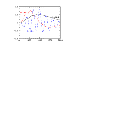
For $BB$ bandpowers, we show the first few eigenvalues and eigenvectors in Figure 1. The main effect of the non-Gaussian covariance is to degrade the variance, by a factor of $\sim 10$, for one KL component which is coherent across a wide range of $l$ and has roughly the same shape as the fiducial $BB$ spectrum. This is consistent with (Smith et al., 2004), in which we found that non-Gaussianity degraded the uncertainty in the overall amplitude of the $BB$ spectrum by a factor of $\sim 10$ when sample variance limited to $l_{\rm max}=2000$. Here we see that this single statement roughly characterizes the entire non-Gaussian covariance between {$TT,TE,EE,BB$} bandpowers.

Figure 1: First three KL eigenmodes, defined by Eq. (27), for the $BB$ power spectrum. These represent modes in $BB$ whose true variance is larger than the variance estimated from Gaussian statistics; the eigenvalue $\lambda$ is the ratio of the two.

IV CMB Lensing Observables

In this section, we quantify the information in terms of the power spectrum of the lenses. An examination of the information contained in the power spectrum of the lenses serves a dual purpose: it is a parameterization independent quantification of the additional information from lensing (§IV.1, IV.2), and it exposes the origin of the non-Gaussian covariance of the CMB as arising from the sample variance of the lenses (§IV.3).

Figure 2: Principal components $K_{1}(l)$, $K_{2}(l)$ of the lensing potential $C_{\ell}^{\phi\phi}$ obtained from CMB measurements to $l_{\rm max}=2000$, as described in §IV.1. These represent modes in the lensing potential which are constrained by measuring either lensed {$T$,$E$} or lensed $B$-modes respectively.

IV.1 Principal Components

We begin by choosing the parameters of interest to be fluctuations $p_{l}$ in the power spectrum of the lenses around the fiducial model

$$C_{l}^{\phi\phi}=(1+p_{l})C_{l}^{\phi\phi}|_{\rm fid}\,.$$ (34)

With these parameters in the Fisher matrix of Eq. (25), the covariance matrix

$$({\bf C})^{ll^{\prime}}=({\bf F}^{-1})^{ll^{\prime}}$$ (35)

can be interpreted as that of the measurements of $C_{l}^{\phi\phi}$ under the assumption that the parameters that control the unlensed CMB are fixed.

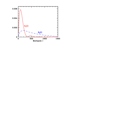
The principal components or eigenvectors of this covariance matrix determine the best constrained linear combinations of $C_{l}^{\phi\phi}$. We find that if lensing $B$-modes are not observed, the covariance ${\bf C}^{ll^{\prime}}$ is dominated by one well-constrained component $K_{1}(l)$, which we show in Figure 2. Equivalently, this means that only one observable in $C_{l}^{\phi\phi}$ is constrained by lensed {$T,E$} power spectra:

$$\Theta_{1}\stackrel{{\scriptstyle\rm def}}{{=}}\sum_{l}{C_{l}^{\phi\phi}\over C_{l}^{\phi\phi}|_{\rm fid}}K_{1}(l).$$ (36)

The power spectrum $C_{l}^{\phi\phi}|_{\rm fid}$ of the fiducial model is scaled out of the weights $K_{1}(l)$, such that deviations from $\Theta_{1}=1$ represent the fractional change in the weighted amplitude of the power. Hence the normalization is chosen such that $\sum_{l}K_{1}(l)=1$.

On the other hand, if we make the artificial assumption that lensing $B$-modes are observed but lensed $\{T,E\}$ are not, then we find that the covariance is dominated by a single broad component $K_{2}$, which peaks at $l\sim 200$ and includes a wide range of $l$. Lensed $B$-mode measurements therefore constrain a second observable

$$\Theta_{2}\stackrel{{\scriptstyle\rm def}}{{=}}\sum_{l}{C_{l}^{\phi\phi}\over C_{l}^{\phi\phi}|_{\rm fid}}K_{2}(l)\,.$$ (37)

The principal components $K_{i}(l)$ were computed assuming cosmic variance limited CMB measurements to $l_{\rm max}=2000$; however, the shape of the eigenmodes remains nearly the same if $l_{\rm max}$ is lowered, or if a white noise power spectrum is used in place of a cutoff in $l$. Therefore, the observables $\Theta_{i}$ provide a parameter-independent representation of the information in the lensed CMB regardless of the noise characteristics. A caveat to this statement is that we never consider CMB multipoles beyond $l_{\rm max}=2000$ in this paper; relaxing this assumption may permit additional modes in the lensing potential to be constrained.

For $BB$, the higher principal components are not completely negligible; the second-best constrained component has a variance which is worse than $K_{2}(l)$ by a factor of 7. We have found that constraints from higher components can almost always be neglected in parameter forecasts, but can have some impact on degenerate directions involving curvature for a measurement of lensing $B$-modes which is close to all-sky cosmic variance limited. In the rest of the paper, we will ignore higher components from lensed $B$-modes.

The structure of the two eigenmodes is related to the lensing kernels of Eq. (6). Given that power in the deflection angles peaks at $l_{1}<100$ in the fiducial model, lensing mainly acts as a convolution kernel of width $l_{1}$ on the high $l$ CMB power spectrum. The {$T,E$} kernels share a similar structure since the angle between the lensed and unlensed ${\bf l}$ is of order $l_{1}/l$. The $B$ kernel is weighted toward higher $l_{1}$ for the same reason. Likewise the dominance of a single mode in {$T,E$} reflects the tight range in $l_{1}$ of the convolution compared with typical structure in the unlensed power spectra.

Figure 3: Redshift sensitivity of the lensing observables $\Theta_{i}$ near the fiducial model. To good approximation the observables constrain the amplitude of $C_{l_{i}}^{\phi\phi}$ around multipoles near the median of the eignmodes of Fig. 2, $l_{K1}=114$, $l_{K2}=440$. The redshift sensitivities $Z_{i}$ at these multipoles (see Eq. (39)) are plotted for the fiducial model.

IV.2 Parameter Sensitivity

Next to understand how sensitivity to these eigenmodes translates into cosmological parameters, let us examine their construction in both the multipole and redshift direction. The change in the observables due to cosmological parameters can be derived from Eqs. (36)-(37) once the change in $C_{l}^{\phi\phi}$ is known.

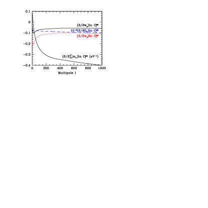
In Fig. 4 we plot the derivatives $\partial C_{l}^{\phi\phi}/\partial p_{\alpha}$ for several cosmological parameters $p_{\alpha}$. The corresponding derivatives of the observables are given in Tab. 2. Since the acoustic peaks constrain

$$l_{A}\stackrel{{\scriptstyle\rm def}}{{=}}{\pi D_{A}(D_{s})/s_{s}}\,,$$ (38)

where $s_{s}$ is the sound horizon at recombination $D_{s}$, we take these derivatives at fixed $l_{A}$ (by adjusting $\Omega_{\rm DE}$). They then quantify the additional sensitivity to cosmological parameters introduced by lensing.

Notice that the derivatives of the power spectra are quite flat compared across the multipoles where the two principal components have support (see Fig. 2). Hence the sensitivity of the observables to most parameters can be accurately determined from the sensitivity of the power spectra at the median multipoles $l_{Ki}$ of the principal components, defined by $\sum_{i=1}^{l_{Ki}}K_{i}(l)=1/2$: $l_{K1}=114$ and $l_{K2}=440$.

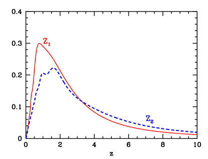
Next, to understand the relative sensitivities to different parameters, consider the fact that $C_{l}^{\phi\phi}$ is determined by a projection of the matter power spectrum with a well-defined redshift sensitivity. In Fig. 3, we plot this sensitivity $Z_{i}(z)$, where

$$C_{l_{K_{i}}}^{\phi\phi}=C_{l_{K_{i}}}^{\phi\phi}|_{\rm fid}\int dzZ_{i}(z)\,.$$ (39)

These weights are calculated under the Limber approximation (see e.g. Hu (2000)). In the fiducial model $\int dzZ_{i}=1$, so that fluctuations in $Z_{i}$ determine fluctuations in the observables as

$$\delta\Theta_{i}\approx{\delta C_{l_{Ki}}^{\phi\phi}\over C_{l_{Ki}}^{\phi\phi}|_{\rm fid}}=\int dz\,\delta Z_{i}(z)\,.$$ (40)

We expect this to be a reasonable approximation since ${\delta C_{l}^{\phi\phi}}$ is not a rapidly varying function of $l$ (see Figure 4).

To make the above considerations more concrete, consider the sensitivity to changes in the distance $D_{A}$, expansion rate $H$, growth rate of the gravitational potential $G$ and the shape of the matter power spectrum $\Delta^{2}_{m}=k^{3}P(k)/2\pi^{3}$ at the lens redshift

$${\delta Z_{i}\over Z_{i}} = \Big{[}n_{i}{\delta D_{A}\over D_{A}}-{\delta H\over H}+2{\delta G\over G}+2{\delta D_{A}(D_{s}-D)\over D_{A}(D_{s}-D)}\Big{]}\,,$$

$$n_{i} \stackrel{{\scriptstyle\rm def}}{{=}} 3-{d\ln\Delta_{m}^{2}\over d\ln k}\Big{|}_{k=({l_{Ki}/D_{A}})}\,.$$ (41)

A typical value for the slope of the power spectrum gives $n_{i}\sim 1$.

CMB lensing is sensitive mainly to high redshift changes in the amount of lensing and correspondingly $\Theta_{1}$ has a median redshift of $z\sim 2$ and $\Theta_{2}$, $z\sim 3$. The observables best constrain cosmological parameters that change the geometry and growth in a coherent fashion at these redshifts. For example, a negative spatial curvature decreases the angular diameter distance to the lens redshifts given the fixed $D_{s}$ and also decreases the growth rate. Both of these effects persist to $z\sim 2-3$ and hence lensing is highly sensitive to the curvature. Likewise massive neutrinos slow the growth from the time they become non-relativistic near recombination. They also create a substantial change at high redshift.

For the dark energy, we take its equation of state to be parameterized by {$w_{0}$, $w_{a}$} according to Eq. (24). These parameters suffer in sensitivity in that the changes they induce on the geometric and growth parameters are dominant at $z<1$. Furthermore their effects on the expansion rate, distance and growth tend to cancel in the observables (see Hu (2005) for a more extended discussion). Note that this a feature of the specific parameter set chosen and may not apply to all dark energy models. The principal component technique allows a parameter independent way of quantifying the lensing information.

The geometric and growth parameters are not the only ones that affect the observables. Since the observables are directly related to the power spectrum of the lenses any parameter that alters it also alters the observables causing parameter degeneracies (see §V). The most important of these are $\Omega_{c}h^{2}$ and the amplitude of the initial power spectrum $\delta_{\zeta}$. The sensitivity of the observables to these parameters are given in Tab. 2. For completeness, we also give the sensitivity to $l_{A}$, though errors on this parameter from the acoustic peaks will be negligible for lensing purposes.

	$\Theta_{1}$	$\Theta_{2}$
$\partial\Theta_{i}/\partial(\sum m_{\nu})$	-0.24	-0.34
$\partial\Theta_{i}/\partial w_{0}$	-0.14	-0.12
$\partial\Theta_{i}/\partial w_{a}$	-0.072	-0.061
$\partial\Theta_{i}/\partial\Omega_{K}$	-8.24	-9.17
$\partial\Theta_{i}/\partial(\Omega_{c}h^{2})$	17.0	24.7
$\partial\Theta_{i}/\partial\ln\,\delta_{\zeta}$	2.00	2.09
$\partial\Theta_{i}/\partial\ln l_{A}$	2.37	2.99

Table 2: Derivatives of the observables $\Theta_{1}$, $\Theta_{2}$ with respect to parameters of interest (top) and nuisance parameters (bottom). In all rows except the last, the derivatives are taken adjusting $\Omega_{\rm DE}$ to hold $l_{A}$ fixed. Units for $\sum m_{\nu}$ are eV.

Figure 4: Derivatives of $C_{l}^{\phi\phi}$ with respect to the parameters $\sum m_{\nu}$, $w_{0}$, $w_{a}$, and $\Omega_{K}$, illustrating the different $l$ dependence. As in Tab. 2, the derivatives are taken adjusting $\Omega_{\rm DE}$ to hold $l_{A}$ fixed.

IV.3 Sample and Noise Variance

The sample and noise variance of the lensing observables determines the errors on cosmological parameters. Furthermore, this characterization of the errors illuminates the origin of the non-Gaussian bandpower covariance.

In Figure 5, we show the $1\sigma$ errors on $\Theta_{i}$ which are obtained for different instrumental sensitivities. Combined with the sensitivity of $\Theta_{i}$ to cosmological parameters, these results may be used to forecast parameter errors (see §V).

Figure 5: Uncertainty on $\Theta_{1}$ from lensed $T$ alone (top) and lensed {$T,E$} (middle), and uncertainty on $\Theta_{2}$ from lensed $B$ (bottom), for varying beam size and noise level $\Delta_{P}$. We assume $\Delta_{T}$ is given by $\Delta_{P}/\sqrt{2}$ throughout, including the top panel. Only multipoles below $l_{\rm max}=2000$ are included. For the zero beam cases, we also show the uncertainties that would be obtained if Gaussian statistics were falsely assumed (dashed). The impact of non-Gaussian contributions is negligible in {$T,E$} but significant for $B$. The horizontal lines are sample variance limits given by Eq. (42).

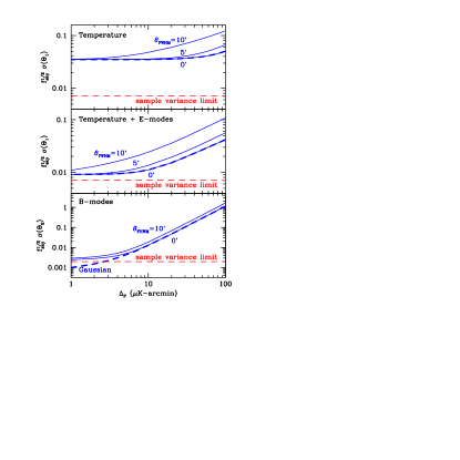
As the instrumental noise goes to zero, the errors saturate at the combined sample variance limits of the lenses and unlensed CMB. To understand the relationship between sample variance and non-Gaussian covariance, consider first an ideal noise-free direct measurement of the lensing potential $\phi$. From the definition (36), the sample variance limit on a measurement of the observables arising from the lenses is given by

$$\sigma^{2}_{\rm SV}(\Theta_{i}) = \sum_{l,l^{\prime}}K_{i}(l)K_{i}(l^{\prime})({\bf C}_{\rm SV})^{ll^{\prime}}$$ (42)

$$= f_{\rm sky}^{-1}\sum_{l}\frac{2}{2l+1}K_{i}(l)^{2}\,.$$

Here we have taken ${\bf C}_{\rm SV}^{ll^{\prime}}=2f_{\rm sky}^{-1}\delta_{ll^{\prime}}/(2l+1)$ under the assumption that $\phi$ is a Gaussian field.

In Figure 5, the sample variance limits of Eq. (42) are shown as dashed horizontal lines. In the limit of zero noise, lensed CMB measurements can measure $\Theta_{1}$ and $\Theta_{2}$ at nearly their sample variance limits. Direct measurements of the $\phi$ field, e.g. from CMB lens reconstruction, do however contain more information than the observables $\Theta_{i}$. They are only two of many quantities that can be constructed with a sample variance limited ${\bf C}_{\rm SV}^{ll^{\prime}}$. These other quantities are related to changes in the shape of $C_{l}^{\phi\phi}$ and may be useful for breaking degeneracies.

The two observables do however contain the majority of the low $l$ information on the amplitude of $C_{l}^{\phi\phi}$. To see this, consider the mode $p_{l}=A-1$ in Eq. (34). This parameter can be measured to

$$\sigma^{2}_{\rm SV}(A)=\left[\sum_{l\leq l_{\phi{\rm max}}}{2l+1\over 2}f_{\rm sky}\right]^{-1}\,.$$ (43)

The qualitative difference between Eqs. (42) and (43) is that the former is limited by the multipoles with the largest weighted sample variance. The latter is limited by the smallest and hence determined by the cutoff $l_{\phi{\rm max}}$. In the fiducial model $\sigma^{2}_{\rm SV}(A)=\sigma_{\rm SV}^{2}(\Theta_{1})$ at $l_{\phi{\rm max}}=198$ and $\sigma^{2}_{\rm SV}(A)=\sigma_{\rm SV}^{2}(\Theta_{2})$ at $l_{\phi{\rm max}}=705$. Given that CMB power spectrum measurements out to $l_{\rm max}=2000$ capture nearly all of the information on the two observables, they also capture essentially all of the information on the amplitude of the lens power spectra near the median of the weights of the eigenmodes.

Finally, if Gaussian statistics are falsely assumed for $BB$, then one would conclude that a high sensitivity measurement of CMB $B$-modes constrains the lensing observable $\Theta_{2}$ better than the sample variance limit (see Fig. 5). From this perspective, one can gain intuition into why non-Gaussianity is significant for lensed $B$-modes. If the $B$-modes were perfectly Gaussian, then the overall amplitude of the lensing could be constrained to within the sample variance of the smallest scale fluctuations in the CMB. In reality, the amplitude of the lensing is limited by the sample variance of the lenses near the median of the eigenvectors, i.e. on degree scales. Band powers below this scale covary in amplitude since the induced $B$-modes share the same lens fluctuations. This covariance becomes noticeable when the intrinsic sample variance of the $E$-modes becomes subdominant due to binning.

The principal component analysis also shows why non-Gaussianity is not a significant limitation for {$T,E$}. The Gaussian errors on $\Theta_{1}$ from observations of lensed {$T,E$} (Fig. 5) never exceed the sample variance limit. This is because the sample variance of the high $l$ unlensed $\{T,E\}$ fields still dominate the measurement of the small fractional changes induced by lensing. The $B$ field does not suffer from this problem in that at high $l$ it is completely generated by lensing.

V Parameter Case Studies

We now study parameter constraints from the lensed CMB, with non-Gaussian contributions to the power spectrum covariance included. In general, parameters which affect the high-redshift universe or the angular diameter distance to last scattering are well measured even without lensing. Lensing mainly helps in breaking degeneracies that leave the observables at recombination fixed. We illustrate this degeneracy breaking with massive neutrinos {$\sum m_{\nu}$}, a constant dark energy equation of state {$w$}, equation of state evolution {$w_{0}$,$w_{a}$}, and spatial curvature {$\Omega_{K}$}. Given that the lensed CMB adds two new observables as described in the previous section, we will study these additional parameters two at a time. We start by examining the {$\sum m_{\nu},w$} case extensively, as an illustration of the impact of non-Gaussianity, as well as a worked example of the use of the lensing observables $\Theta_{i}$.

	$\nu$	$\theta_{\rm FWHM}$	$\Delta_{T}$	$\Delta_{P}$	$f_{\rm sky}$
Planck	100 GHz	$9.2^{\prime}$	51	–	0.8
	143 GHz	$7.1^{\prime}$	43	78	0.8
	217 GHz	$5.0^{\prime}$	65	135	0.8
Deep10%	–	1.0’	1.00	1.41	0.1

Table 3: Assumed experimental specifications for the reference survey in §V, consisting of Planck and a deep polarization field with 10% of sky. The noise parameters $\Delta_{T}$ and $\Delta_{P}$ are given in units of $\mu$K-arcmin. For the combined reference survey, $\sigma(\Theta_{1})=0.025$ and $\sigma(\Theta_{2})=0.008$.

Throughout this section, we will consider a reference survey (Tab. 3) which consists of Planck measurements on most of the sky, combined with a smaller deep survey which measures lensing of the temperature and polarization with higher signal-to-noise. (We assume that the deep survey area is a subset of the Planck survey area.)

V.1 Neutrinos and constant equation of state

We consider here the constraints in the {$\sum m_{\nu},w$} plane at fixed $\Omega_{K}$ employing a direct Fisher matrix forecast in the parameter space and through the intermediary measurement of the lensing observables, first by adding its information to the unlensed spectra in the full parameter space and then by pre-marginalizing parameters that control the high redshift physics at recombination.

V.1.1 Direct forecasts

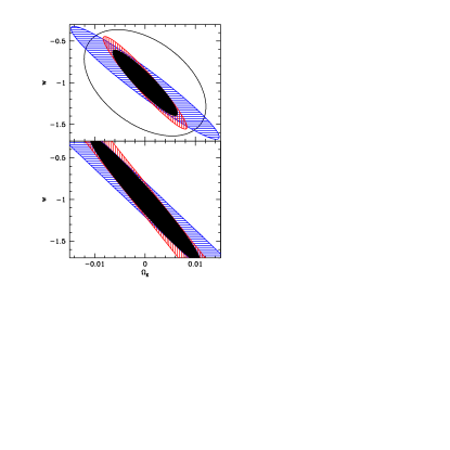
In Figure 6, left panels, we show the constraints falsely assuming Gaussian statistics. For illustrative purposes, we first show the errors with the parameters {$\Omega_{c}h^{2}$, $\ln\,\delta_{\zeta}$}, fixed to their fiducial values (top left), but with the remaining parameters {$\Omega_{\rm DE}$, $\Omega_{b}h^{2}$, $\tau$, $n_{s}$, $r$} marginalized. As we shall see, the former two parameters affect the lensing observables and cause degeneracies with the parameters of interest.

The large surrounding ellipse in the top left panel represents the double angular diameter distance degeneracy expected from the unlensed CMB. Adding information from lensed {$T,E$} (horizontally shaded) constrains a slightly different combination of degenerate parameters than adding information from lensed $B$ (vertically shaded). This is because changes in the two parameters {$\sum m_{\nu},w$} affect $C_{l}^{\phi\phi}$ differently in $l$ (Fig. 4) and hence the two lensing observables described in §IV.

Figure 6: Degeneracy breaking in the $\sum m_{\nu}-w$ plane from CMB lensing, for the reference survey in Tab. 3. Ellipses here and throughout are plotted at $\Delta\chi^{2}=1$ and not 68% CL. In each panel, the surrounding ellipse represents parameter constraints from unlensed {$T,E$}, the blue/horizontally-shaded ellipse represents constraints from lensed {$T,E$}, the red/vertically-shaded ellipse represents constraints from unlensed {$T,E$} + lensed $B$, and the inner solid ellipse represents constraints from lensed {$T,E,B$}. In the top panels, we show Gaussian (top left) and non-Gaussian (top right) constraints with {$\Omega_{c}h^{2},\ln\,\delta_{\zeta}$} held fixed, and the remaining parameters {$\Omega_{b}h^{2},\Omega_{\rm DE},\tau,n_{s},r$} marginalized. In the bottom panels, we show Gaussian (bottom left) and non-Gaussian (bottom right) constraints with all parameters marginalized.

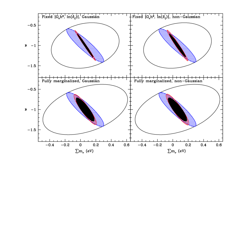
We next consider the effect of including the non-Gaussian covariance, in the top right panel of Fig. 6. Compared to Gaussian uncertainties, the constraints from lensed {$T,E$} are unaffected (as expected from §III.2), while constraints from lensed $B$ are degraded for the best constrained combination of the two parameters. Note that because we have considered a nearly degenerate two parameter space, even here the effect of non-Gaussianity is hidden from the errors on a single parameter marginalized over the other.

However, the discussion so far has assumed perfect priors for the parameters {$\Omega_{c}h^{2},\ln\,\delta_{\zeta}$}. If these are marginalized with only information from the reference survey, the effect of non-Gaussianity is overwhelmed by the effect of marginalizing (see Fig. 6, bottom panels). This is true even if $B$ were the only source of lensing information or if there were only one additional parameter.

Nonetheless the effect of non-Gaussianity in the full parameter space is not negligible; it does enlarge the volume which is allowed. The enlargement occurs along a direction which is a combination of several parameters {$\Omega_{c}h^{2},\ln\,\delta_{\zeta},w,\sum m_{\nu}$}. Though hidden by marginalization, this degradation can be exposed if there are external prior measurements of other combinations of these parameters. It can also reduce the apparent goodness of fit to the best-fit model (see Appendix A). Finally for different reference surveys, e.g. a smaller but deeper survey, a Gaussian assumption can again give a misleading answer on the utility of the $B$-modes (see §VI).

These results can be reproduced and understood using the lensing observables $\Theta_{i}$ as we shall now see.

Figure 7: Forecasted errors in {$\sum m_{\nu},w$} as in Fig. 6 (lower right panel, non-Gaussian, fully marginalized) but with the additive lensing observables prescription from §V.1.2. Note the excellent agreement between the direct and observables approaches.

V.1.2 Additive observables forecasts

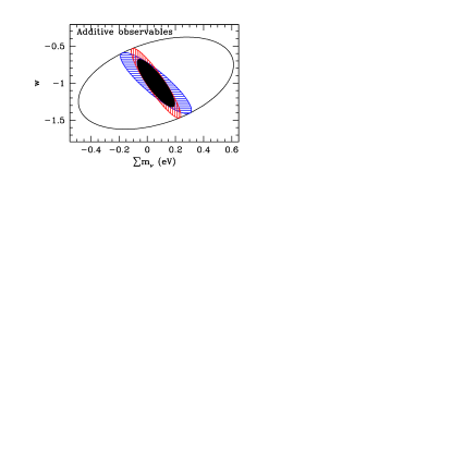
The lensing observables provide a general framework for forecasting the additional constraints supplied by lensing in any parameter space. We can use the direct forecasts from the preceding section as a basis for comparison with the following construction:

1. From the parameters of the survey under consideration (sky coverage, noise, and beam), compute uncertainties (see Fig. 5) on the observables $\Theta_{i}$ and assume they are independent, obtaining a 2$\times$2 covariance matrix:

   $$\mbox{Cov}(\Theta_{i},\Theta_{j})=\left(\begin{array}[]{cc}\sigma^{2}(\Theta_{1})&0\\ 0&\sigma^{2}(\Theta_{2})\end{array}\right)\,.$$ (44)

2. Transform these parameter errors into a Fisher matrix in the desired parameter space with

   $$F_{\alpha\beta}^{\rm lens}=(\partial_{\alpha}\Theta^{i})\mbox{Cov}(\Theta_{i},\Theta_{j})^{-1}(\partial_{\beta}\Theta^{j})\,$$ (45)

   and add this to the Fisher matrix of the unlensed CMB or any external data set.

Some of the more common parameter derivatives for use in Eq. (45) are given in Tab. 2. Others can be approximated by evaluating $C_{l}^{\phi\phi}$ at the median multipole. An advantage of the observables scheme is that it automatically includes the effect of non-Gaussianity without reference to the bandpower covariance matrix. One simply uses the non-Gaussian errors from Fig. 5.

The main caveat to the observables prescription is that it implicitly assumes that lensing is an additive source of information. It should not be used to forecast parameters for which lensing destroys information such as tensors or features in the initial power spectrum. In the particular case of the tensor-to-scalar ratio $r$, we find that non-Gaussianity in the lensed CMB is always negligible when forecasting uncertainties, even when low-redshift parameters are marginalized.

We show the $w-\sum m_{\nu}$ example in Fig. 7. Note the excellent agreement with the direct Fisher calculation in Fig. 6 (lower right panel) in all respects.

V.1.3 Nuisance-marginalized observables

This prescription can be further simplified so as not to require computation of the unlensed CMB Fisher matrix or external information for forecasting parameter errors which rely mainly on the lensing information. In this case the extra information is utilized to remove the parameter degeneracy from $\Omega_{c}h^{2}$ and $\ln\,\delta_{\zeta}$ in the observables $\Theta_{i}$. These parameters can be premarginalized and dropped from the Fisher matrix constructed from $\Theta_{i}$.

Operationally, to pre-marginalize the nuisance parameters, we add the “nuisance errors”

$$\mbox{Cov}_{\rm nuis}(\Theta_{i},\Theta_{j}) \stackrel{{\scriptstyle\rm def}}{{=}} \frac{\partial\Theta_{i}}{\partial\Omega_{c}h^{2}}\frac{\partial\Theta_{j}}{\partial\Omega_{c}h^{2}}\sigma^{2}(\Omega_{c}h^{2})$$

$$\qquad+\,\frac{\partial\Theta_{i}}{\partial\ln\,\delta_{\zeta}}\frac{\partial\Theta_{j}}{\partial\ln\,\delta_{\zeta}}\sigma^{2}(\ln\,\delta_{\zeta})$$

to the “measurement errors” defined by Eq. (44), to get an effective covariance matrix $\mbox{Cov}_{{\rm eff}}=(\mbox{Cov}+\mbox{Cov}_{\rm nuis})$. We then use $\mbox{Cov}_{{\rm eff}}$ instead of Cov in Eq. (45), to obtain a Fisher matrix in a parameter space where {$\Omega_{c}h^{2},\ln\,\delta_{\zeta}$} is excluded.

In (V.1.3), we have neglected the correlations between $\Omega_{c}h^{2}$ and $\ln\,\delta_{\zeta}$ but these provide a negligible effect if the source of information is internal to the CMB. Note that $\mbox{Cov}_{{\rm eff}}$ will typically show a high degree of correlation between the two observables since the increase in the effective errors is along directions that are degenerate with the two parameters. For parameters that do not induce a degenerate change, this correlation reflects extra information (see §VI.2).

	WMAP3	Planck	Reference	Ideal
$\sigma(\Theta_{1})$	-	0.050	0.025	0.0089
$\sigma(\Theta_{2})$	-	-	0.008	0.0023
$\sigma(\Omega_{c}h^{2})$	0.01	0.0011	0.0009	0.0005
$\sigma(\ln\,\delta_{\zeta})$	0.03	0.0045	0.0040	0.0023
$\sigma_{\rm nuis}(\Theta_{1})$	0.18	0.020	0.017	0.0094
$\sigma_{\rm nuis}(\Theta_{2})$	0.25	0.028	0.023	0.011
$\mbox{Corr}_{\rm nuis}(\Theta_{1},\Theta_{2})$	0.99	0.99	0.99	0.99
$\sigma_{{\rm eff}}(\Theta_{1})$	-	0.054	0.030	0.013
$\sigma_{{\rm eff}}(\Theta_{2})$	-	-	0.025	0.013
$\mbox{Corr}_{{\rm eff}}(\Theta_{1},\Theta_{2})$	-	-	0.52	0.71

Table 4: Uncertainties in lensing observables from third-year WMAP Spergel et al. (2006), Planck alone (Tab. 3, top), the reference experiment consisting of both parts of Tab. 3, and an ideal survey which is all-sky cosmic variance limited in temperature and polarization to $l_{\rm max}=2000$. Top: Measurement errors on the lensing observables {$\Theta_{1},\Theta_{2}$} computed from the raw sensitivity to lensed {$T,E$} and $B$ respectively, as in Fig. 5. Middle: “Nuisance” errors of Eq. (V.1.3) on lensing observables, computed by propagating each survey’s unlensed uncertainties on {$\Omega_{c}h^{2},\ln\,\delta_{\zeta}$} (also shown) using derivatives from Tab. 2. Bottom: Total errors on lensing observables, computed by adding 2$\times$2 covariance matrices ($\mbox{Cov}_{{\rm eff}}=\mbox{Cov}+\mbox{Cov}_{\rm nuis}$). As described in the text, these are the effective errors on lensing observables when constraining low-redshift parameters with nuisance parameters {$\Omega_{c}h^{2},\ln\,\delta_{\zeta}$} premarginalized.

Let us illustrate this pre-marginalization scheme for {$\sum m_{\nu},w$} and the reference survey. For comparison with Fig. 6, we will compute errors with priors on {$\Omega_{c}h^{2},\ln\,\delta_{\zeta}$} that fix them completely, and priors that are derived from determinations internal to the reference survey (see Tab. 4). The former case also corresponds to using Cov (Eq. (44)) in place of $\mbox{Cov}_{{\rm eff}}$. Combined with the parameter derivatives from Tab. 2, the result of this procedure is shown in Fig. 8.

The constraints agree well with the direct Fisher calculation in the right panels of Fig. 6 along the best constrained direction. For example, with $\sum m_{\nu}$ fixed, the uncertainty $\sigma(w)$ is 0.150 from the direct Fisher calculation (§V.1.1), 0.170 from the additive-observables prescription (§V.1.2), and 0.178 from the premarginalized-observables prescription described in this section. In practice, the main difference between the last two is that in the premarginalized-observables prescription, the constraints computed are from lensing alone; information from the unlensed CMB which helps constrain intermediate-redshift parameters (such as ISW) is not included.

A pedagogical advantage of pre-marginalization is that it clarifies the limiting source of uncertainty. For example, in our reference survey, $\sigma_{\rm nuis}(\Theta_{2})$ is substantially larger than $\sigma(\Theta_{2})$. The utility of the lensing observable is therefore limited by the nuisance parameters and not by the sample or noise variance on lensing. This also explains the negligible impact of non-Gaussian sample variance on marginalized parameter errors in Fig. 6.

Figure 8: Forecasted errors in {$\sum m_{\nu},w$} as in Fig. 6 (right panels, non-Gaussian) but with the premarginalized-observables prescription from §V.1.3. The blue/horizontally-shaded regions show only the $\Theta_{1}$ constraint from lensed {$T,E$}, the red/vertically-shaded regions show only the $\Theta_{2}$ constraint from lensed $B$, and the solid regions show the combined constraint from both observables. The top panel shows the case where {$\Omega_{c}h^{2},\ln\,\delta_{\zeta}$} are completely fixed by the external prior; the bottom panel shows the case where the parameters are internally determined by the reference survey itself.

V.2 Evolution of equation of state

We now consider CMB constraints on a time-dependent dark energy equation of state through {$w_{0},w_{a}$} [see Eq. (24)]. For purposes of this subsection, we assume that both the neutrino mass and spatial curvature are fixed and marginalize {$\Omega_{\rm DE}$, $\Omega_{b}h^{2}$, $\Omega_{c}h^{2}$, $\tau$, $n_{s}$, $r$}.

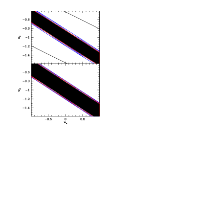
In Fig. 9, we show errors on $w_{0}$ and $w_{a}$, for the reference survey of Tab. 3, using the premarginalized observables scheme from §V.1.3. In the top panel we show the direct Fisher matrix calculation for comparison. One parameter combination is constrained by CMB lensing, but the complementary direction is degenerate, acquiring CMB constraints only from the unlensed CMB through the ISW effect (c.f. Acquaviva and Baccigalupi (2005)).

The {$w_{0},w_{a}$} degeneracy can be seen directly by noting that the $w_{0}$ and $w_{a}$ derivatives, taken at constant angular diameter distance, of $C_{l}^{\phi\phi}$ are nearly proportional (Fig. 4), so that a parameter space direction exists which preserves both $C_{l}^{\phi\phi}$ and the unlensed CMB. This is also seen in Tab. 2, where the $w_{0}$ and $w_{a}$ derivatives of {$\Theta_{1},\Theta_{2}$} are nearly proportional.

The degeneracy can be interpreted as the statement that the lensed CMB constrains $w(z)$ mainly around the pivot redshift $z_{p}\sim 1$ with uncertainty $\sigma(w_{p})=0.15$ for the reference survey. The pivot redshift can be interpreted as a combination of the high redshift weight of CMB lensing discussed in §IV.2 and the dark energy parameters which change observables strongly only at $z<1$. Note that this pivot redshift is substantially higher than many other cosmological probes and implies that CMB lensing will provide complementary constraints on the evolution of the equation of state. We also note that the pivot redshift and $\sigma(w_{p})$ will depend on the underlying fiducial model.

Figure 9: Joint uncertainties on dark energy parameters {$w_{a},w_{0}$}, for the reference survey in Tab. 3, with {$\sum m_{\nu},\Omega_{K}$} fixed to their fiducial values and all other parameters marginalized. The top panel shows the direct Fisher matrix calculation; the bottom panel shows errors calculated using the premarginalized-observables scheme (§V.1.3). In this parameter space, the lensing observables are degenerate; the $\Theta_{1}$ constraints (blue/horizontally-shaded), the $\Theta_{2}$ constraints (red/vertically-shaded), and the combined constraints (solid) are nearly identical. Given this nearly perfect degeneracy, the Fisher forecast should not be interpreted literally along the full extent of the degeneracy.

V.3 Curvature

Given the sensitivity of CMB lensing to changes at high redshift, constraints on spatial curvature are much stronger than those on the dark energy when compared with low-redshift probes of the expansion history. In Fig. 10, we show the reference constraints in the {$\Omega_{K},w$} plane with {$\Omega_{b}h^{2},\Omega_{c}h^{2},\Omega_{\rm DE},\tau,n_{s},r$} marginalized and {$\sum m_{\nu},w_{a}$} fixed.

The two observables are again nearly degenerate in this plane. The direction of the degeneracy is well but not perfectly matched in the observables scheme for the case of $\Theta_{1}$. The reason for this is that the unlensed CMB carries information on the curvature both from the ISW effect and from the intrinsic sharpness of the acoustic peaks (see Hu and White (1996), Fig. 11). The latter effect comes from the geometrical projection of $k$-space power to $l$-space through the radial eigenfunctions. Unlike lensing this effect smooths (negative curvature) or sharpens (positive curvature) even the low order peaks as it is associated with the curvature across the last scattering surface as a whole. For the high order peaks it destructively interferes with the lensing effect and mildly violates the assumption that lensing is an independent additive source of information. The interference and the rotation it causes however are small and, if desired, can be accounted for by a $\sim 20\%$ lowering of $\partial\Theta_{1}/\partial\Omega_{K}$ for surveys that utilize information near $l_{\rm max}=2000$.

More importantly, the direction that is well constrained has a large $\Omega_{K}$ and only a small $w$ component, i.e. the degeneracy is very steep in the curvature direction. The implication is that it takes only a weak external constraint on $w$ to break this degeneracy completely. When combined with other dark energy probes, the lensing observables can be thought of as fixing the curvature. We explore this use of CMB lensing further in a separate piece Hu et al. (2006).

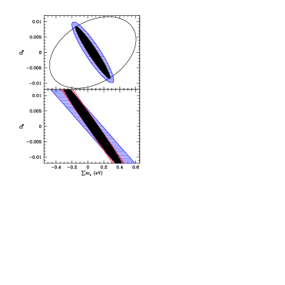
Even given other probes that break the {$\Omega_{K},w$} degeneracy, $\Omega_{K}$ remains nearly degenerate with $\sum m_{\nu}$. In Fig. 11, we show constraints in this plane with {$w_{0},w_{a}$} fixed. The observables approach again accurately models the well constrained direction aside from the slight rotation of the $\Theta_{1}$ constraint which makes curvature nearly perfectly degenerate with neutrinos. Breaking this degeneracy externally will require independent probes with limits of $\sigma(\Omega_{K})\ll 0.005$ (perhaps with measurements of the angular diameter distance to $z\sim 3$ Knox (2006)) or $\sigma(\sum m_{\nu})\ll 0.2$eV.

Figure 10: Joint uncertainties on {$\Omega_{K},w_{0}$}, for the reference survey of Tab. 3, with {$\sum m_{\nu},w_{a}$} fixed to their fiducial values and all other parameters marginalized. The top panel shows the direct Fisher matrix calculation; the bottom panel shows errors calculated using the premarginalized-observables scheme from §V.1.3. As expected, the two agree in the well constrained direction, but the second scheme overestimates the errors in the poorly constrained, ISW-limited, direction.

Figure 11: Joint uncertainties on dark energy parameters {$\sum m_{\nu},\Omega_{K}$} with {$w_{0},w_{a}$} fixed to their fiducial values. for the reference survey of Tab. 3, using the direct Fisher calculation (top panel) and the premarginalized-observables scheme (bottom panel). (In the top panel, the red/vertically-shaded ellipse representing unlensed {$T,E$} and lensed $B$ is hidden by the solid ellipse representing lensed {$T,E,B$}.)

VI Survey Optimization

In the previous section, we quantified the information supplied by CMB lensing in the context of a specific reference survey. We conclude this paper by considering how surveys can optimize the extraction of cosmological information from lensed power spectra.

VI.1 $\Omega_{c}h^{2}$, $\tau$, and $l_{\rm max}$

We have seen in §IV that imperfect knowledge of {$\Omega_{c}h^{2}$, $\ln\,\delta_{\zeta}$} results in nuisance errors which limit the ability to extract cosmological information from lensing. The nuisance errors $\sigma_{\rm nuis}(\Theta_{i})$ represent a floor below which improving sensitivity to each lensing observable individually does not improve cosmological parameter constraints. More precisely, improving $\sigma(\Theta_{i})$ beyond this level will correlate low-redshift parameters to {$\Omega_{c}h^{2},\ln\,\delta_{\zeta}$}, in such a way that marginalized uncertainties do not improve if only one of the observables is measured. Joint measurement can slightly improve on this “floor” due to the difference in how the nuisance parameters affect the two.

One source of nuisance error arises from uncertainty in $\Omega_{c}h^{2}$ as measured from the primary CMB or external data. This is the dominant source of error throughout Tab. 4, in which we have assumed that the range of multipoles from which cosmology can be extracted is limited to $l_{\rm max}=2000$. This cut reflects an estimate of possible contamination from other secondaries and foregrounds and is currently uncertain. Fortunately the dependence of $\sigma(\Omega_{c}h^{2})$ on $l_{\rm max}$ is not particularly sensitive strong (see Fig. 12), provided that it exceeds the knee at $l_{\rm max}\sim 700$, corresponding to the trough between the second and third acoustic peaks.

Figure 12: Uncertainty $\sigma(\Omega_{c}h^{2})$ from CMB measurements with varying $l_{\rm max}$, for Planck sensitivity (Tab. 3), and ideal measurement of unlensed CMB temperature and polarization.

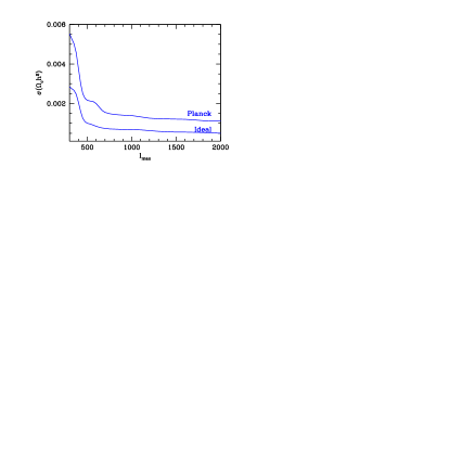
Another conclusion from Fig. 12 is that achieving cosmic variance limited measurement of $E$-mode acoustic peaks at intermediate $l$ would significantly improve $\Omega_{c}h^{2}$ constraints from Planck. For example, an ideal measurement of {$T,E$} with $l_{\rm max}\sim 500$ would obtain $\Omega_{c}h^{2}$ constraints comparable to Planck, even though Planck will measure CMB temperature anisotropy well into the damping tail. We have found that the inability to extract $\Omega_{c}h^{2}$ constraints from the temperature damping tail is due to confusion with the spectral index $n_{s}$; if $n_{s}$ is fixed rather than marginalized, then Planck’s $\Omega_{c}h^{2}$ constraints significantly improve.

As $l_{\rm max}$ is increased in Fig. 12, the error on $\Omega_{c}h^{2}$ improves, but the error on our second nuisance parameter $\ln\,\delta_{\zeta}$ stays nearly constant. This is because the degeneracy between $\ln\,\delta_{\zeta}$ and $\tau$ in the unlensed CMB is broken only by the reionization signal at low polarization multipoles. Even at $l_{\rm max}=2000$, the largest value we consider in this paper, the nuisance errors are dominated by uncertainty in $\Omega_{c}h^{2}$. This may suggest that $\ln\,\delta_{\zeta}$ is never important as a nuisance parameter. There are three reasons why this may not be the case in practice.

First, errors on $\Omega_{c}h^{2}$ can be in principle be improved over CMB determinations by external sources such as weak lensing of galaxies or even from the CMB itself through lens reconstruction, whereas amplitude uncertainties from reionization will likely remain. Second, we assume that large angle polarization foregrounds can be perfectly removed to the cosmic variance limit through the frequency channels not used for cosmology. These foregrounds are now known to dominate the polarization signal in all bands Spergel et al. (2006).

Third, our parameter forecasts so far have implicitly assumed sharp reionization, characterized by the single parameter $\tau$, the total optical depth to recombination. More general models of reionization can include additional parameters which degrade uncertainties on $\tau$ Kaplinghat et al. (2003b); Holder et al. (2003), and therefore our nuisance parameter $\ln\,\delta_{\zeta}$, beyond what is shown in Tab. 4.

If we conservatively assume that the ionization history takes an arbitrary form, uncertainties rise to $\sigma(\tau)=\sigma(\ln\,\delta_{\zeta})=0.01$ Hu and Holder (2003) and by Tab. 2, the corresponding nuisance errors are $\sigma_{\rm nuis}(\Theta_{1})=\sigma_{\rm nuis}(\Theta_{2})=0.02$. Comparing with Tab. 4, this would be a comparable source of nuisance error to $\Omega_{c}h^{2}$ for Planck, and would represent the dominant uncertainty for an ideal experiment that achieves cosmic variance on the $E$-modes (c.f. Fig. 12).

Finally the choice of $l_{\rm max}$ also affects constraints on $\Theta_{1}$. For example scaling back to $l_{\rm max}=1500$ would degrade $\sigma(\Theta_{1})$ by $1.2$ for Planck and $1.6$ for the ideal measurement.

VI.2 Optimizing sensitivity to lensing $B$-modes

An important issue for upcoming polarization experiments is optimizing sky coverage with the total integrated sensitivity fixed. In general this is not a well-posed question since the sky coverage can be optimized with respect to systematic errors, foreground contamination, sensitivity to the $E$-mode power spectrum, sensitivity to tensor $B$-modes, detection of lensing $B$-modes, $B$-mode reconstruction of the lensing fields, or sensitivity to cosmological parameters from the $B$-mode power spectrum. Here, we consider only the last of these, with particular attention to how optimizing the sensitivity is affected by non-Gaussian statistics.

The integrated sensitivity $\mu$ has units of temperature and is given by $\nu/\sqrt{NT}$ where $\nu$ is the instantaneous sensitivity (in mK$\sqrt{\mbox{sec}}$) per Stokes parameter per detector, $N$ is the number of detectors, and $T$ is the total integration time. The noise variance per steradian in Eq. (15) is then given by $\Delta_{P}=\mu\sqrt{A}$ where $A$ is the survey area in steradians.

In §IV, we found that all cosmological constraints from the lensing $B$-mode power spectrum are derived from the single observable $\Theta_{2}$. Therefore, there is a natural figure of merit for optimizing sky coverage: the $1\sigma$ error $\sigma(\Theta_{2})$. In Fig. 13, we show $\sigma(\Theta_{2})$ for varying $f_{\rm sky}$, assuming fixed integrated sensitivity $\mu=2$ nK. Incorporating non-Gaussian statistics increases the optimal value of $f_{\rm sky}$ by a factor of 3 relative to Gaussian, and significantly steepens the dependence of $\sigma(\Theta_{2})$ on $f_{\rm sky}$ in a manner which disfavors small $f_{\rm sky}$.

Figure 13: Dependence of the figure of merit $\sigma(\Theta_{2})$ on $f_{\rm sky}$, for fixed integrated sensitivity $\mu=2$ nK. The solid line shows the result using non-Gaussian statistics for lensed $B$-modes (§II); the dashed line shows the result if Gaussian statistics are falsely assumed. The horizontal lines represent the “nuisance” errors on $\Theta_{2}$ from imperfect measurement of {$\Omega_{c}h^{2}$, $\ln\,\delta_{\zeta}$}, for Planck and for ideal measurement of the unlensed CMB (Tab. 4).

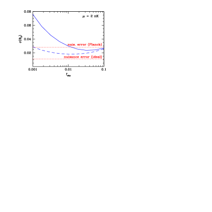
We have shown the $f_{\rm sky}$ optimization in detail for integrated sensitivity $\mu=2$ nK; in general, the optimal $f_{\rm sky}$ will scale with $\mu$ as $f_{\rm sky}\propto\mu^{-2}$. The same scaling is obtained assuming either Gaussian or non-Gaussian statistics; therefore, the optimal patch size with non-Gaussian statistics incorporated is a factor of 3 larger than the Gaussian value, independent of the integrated sensitivity. Another way of stating the optimality criterion is: the optimal patch size is always chosen so that the noise per steradian takes the value

$$(\Delta_{P})_{\rm optimal}=4.7\mbox{ $\mu$K-arcmin}.$$ (47)

This criterion makes no reference to the value of $\mu$ but does assume zero beam; we have found that $(\Delta_{P})_{\rm optimal}$ is nearly independent of beam size, provided that $\theta_{\rm FWHM}\leq 15$ arcmin. (We note that if Gaussian statistics were falsely assumed for lensing $B$-modes, then one would obtain $(\Delta_{P})_{\rm optimal}=2.8$ $\mu$K-arcmin.)

Another conclusion of the previous section was that, for sufficiently precise measurements of lensing $B$-modes, the ability to extract cosmological information from the CMB alone is primarily limited by uncertainty in $\Omega_{c}h^{2}$ from the primary CMB and secondarily limited by reionization if the ionization history is complex. More precisely, when the measurement error $\sigma(\Theta_{2})$ becomes as good as the the nuisance error $\sigma_{\rm nuis}(\Theta_{2})$, then improved sensitivity to lensing $B$-modes serves mainly to correlate low-redshift and nuisance parameters, rather than improving marginalized uncertainties on either. In Fig. 14, we have shown the dependence of $\sigma(\Theta_{2})$ on total sensitivity and sky coverage.

Figure 14: Level contours for the figure of merit $\sigma(\Theta_{2})$ in the $f_{\rm sky}$-$\mu$ plane, assuming zero beam.

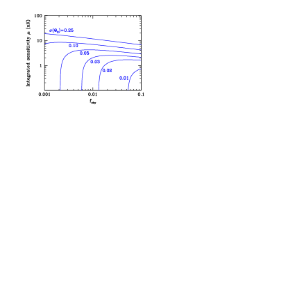
We now consider optimization of a deep ground-based polarization survey designed to complement Planck. For the Planck prior on $\Omega_{c}h^{2}$, we found $\sigma_{\rm nuis}(\Theta_{2})=0.028$ (Tab. 4). Comparing with Fig. 14, it is seen that a narrow-beam polarization survey with integrated sensitivity $\mu$=1-2 nK, and covering a few percent of the sky, will achieve $\sigma(\Theta_{2})\approx\sigma_{\rm nuis}(\Theta_{2})$ and is therefore nearly optimal for extracting cosmological information from lensing $B$-modes alone, within the limits of the Planck prior.

Figure 15: Uncertainty on the single low-redshift parameter $w$, marginalized over high-redshift parameters, for Planck complemented by a deep survey with varying sky coverage $f_{\rm sky}$. For the deep survey, we assume $\Delta_{T}=\Delta_{P}/\sqrt{2}$ and consider three sensitivity levels as indicated.

Unmarg.	Lensed Planck	Planck+Deep5%	Reference	Ideal
$\sigma(w_{0})$	0.31	0.18	0.15	0.07
$\sigma(w_{a})$	0.65	0.38	0.30	0.15
$\sigma(\Omega_{K})$	0.0076	0.0032	0.0025	0.0013
$\sigma(\sum m_{\nu})$	0.20	0.085	0.063	0.032

Table 5: Uncertainties on each of {$w_{0},w_{a},\Omega_{K},\sum m_{\nu}$} separately with the others fixed, and high-redshift parameters marginalized. Here, “Deep_5%” stands for a deep survey with $f_{\rm sky}=0.05$, zero beam, and $\Delta_{P}=\sqrt{2}\Delta_{T}=4.7$ $\mu$K-arcmin (see Eq. (47)). The reference survey is as in §V and covers $f_{\rm sky}=0.10$, and “Ideal” refers to all-sky cosmic variance limited {$T,E,B$} to $l_{\rm max}=2000$. Forecasts here are from the direct Fisher approach.

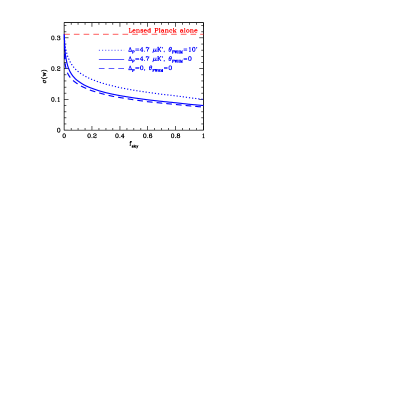
This conclusion that a few percent of the sky is optimal for extracting the $B$-mode information alone is slightly modified once the $T$ and $E$ information from Planck and the deep ground-based survey itself are considered. The $T$ and $E$ measurements supply $\Theta_{1}$ and the nuisance parameters. The first modification is that if Planck succeeds in measuring $\Theta_{1}$ to the forecasted $\sigma(\Theta_{1})=0.05$ then it alone has lensing information that is comparable to an $f_{\rm sky}\sim 0.01$ $B$-mode survey. The second modification is that as the deep survey improves the nuisance parameters directly or through $\Theta_{1}$, the nuisance floor on the $B$-modes correspondingly drops. Both considerations favor slightly larger $f_{\rm sky}$. To illustrate this we show in Fig. 15 the direct forecast on a single low-redshift parameter, e.g. $w$, if Planck is complemented by a deep survey with varying $f_{\rm sky}$. For $f_{\rm sky}$ less than the “knee” at $f_{\rm sky}\sim 0.05$, the uncertainty in $w$ from the $B$-mode measurement itself improves as $f_{\rm sky}^{-1/2}$ but only becomes stronger than the lensing constraint from Planck for $f_{\rm sky}\gtrsim 0.01$. For $f_{\rm sky}\gtrsim 0.05$ improvements scale more slowly as $\sim f_{\rm sky}^{-1/3}$. Half the total improvement comes from $f_{\rm sky}<0.1$. In fact, a deep survey with $f_{\rm sky}=0.05$ can improve Planck lensing uncertainties on any one of {$w_{0},w_{a},\Omega_{K},\sum m_{\nu}$}, with the others fixed, by a factor of $\sim 2$ (Tab. 5) through measurement of the $B$-mode observable. Moreover if lensing constraints from Planck prove impossible to extract due to foreground and secondary contamination this improvement represents another factor of $\sim 2$ in errors.

VII Discussion

We have provided a comprehensive study of the additional cosmological information supplied by lensed power spectra of the CMB temperature and polarization fields including the non-Gaussian covariance between bandpower estimates. This covariance originates from the sample variance of the degree scale lenses on the CMB fields at smaller scales. It is nearly irrelevant for the temperature and $E$-polarization fields out to $l_{\rm max}=2000$ due to the larger sample variance of the unlensed CMB. For the amplitude of the $B$-polarization field, it increases the variance by up to a factor of $\sim 10$ and changes the optimal observing strategy to one that covers a factor of $\sim 3$ times more sky area.

The impact of non-Gaussianity on parameter estimation as well as the net information content of the lensed spectra is more subtle. These answers depend on the choice of parameters and the external priors associated with them. We have provided a framework of lensing observables that greatly simplifies these examinations.

In this framework, lensed CMB power spectra provide information on only two observables, one which determines the lens power spectra at $l\sim 100$ associated with the {$T,E$}-fields and one which determines it at $l\sim 500$ associated with the $B$-field. The observables are constructed from the principal components of the lensing power spectrum $C_{l}^{\phi\phi}$. Non-Gaussianity is then automatically incorporated in the errors on the observables which will eventually approach, but never exceed, the sampling errors of the lenses as the measurements improve.

This construction also illuminates the origin of parameter degeneracies which can rapidly become the limiting source of uncertainties for parameters of interest. Any combination of parameters that leaves the lensing observables and the CMB at recombination fixed within the errors cannot be determined. To illustrate these effects, we have isolated two parameters $\Omega_{c}h^{2}$ and $\ln\,\delta_{\zeta}$ that determine the shape and amplitude of the matter power spectrum respectively, and marginalized their uncertainties assuming internal CMB determinations of each from the Planck satellite. These become the limiting uncertainties once the observables are determined to the several percent level and are only slowly improved as the lensing survey itself improves the nuisance errors. While $\Omega_{c}h^{2}$ constraints can be improved externally to the CMB, those on $\ln\,\delta_{\zeta}$ are more difficult to improve and may be limited by our understanding of reionization.

There are also degeneracies within the space of the parameters of interest that control the expansion rate and growth of structure at intermediate redshifts. When taken one at a time, uncertainties on the parameters {$w_{0},w_{a},\Omega_{K},\sum m_{\nu}$} can be improved by a factor of $\sim 2-3$, relative to Planck alone, by a deep ground-based polarization survey on 5-10% of the sky. However {$w_{0},w_{a}$} are nearly perfectly degenerate in the lensing observables as are {$\Omega_{K},\sum m_{\nu}$} separately. The degeneracy between two parameters in each pair is weakly broken by the two observables. For example, when errors on $\sum m_{\nu}$ are marginalized over $w_{0}$ they degrade by a factor of 2 for the reference survey (see Fig. 6). However sensitivity to the {$\Omega_{K},\sum m_{\nu}$} pair is much greater than to the dark energy parameters due to the high redshift weights of the lensing observables. When combining lensed CMB power spectra with other more incisive probes of the dark energy, lensing essentially fixes one well-defined combination of {$\Omega_{K},\sum m_{\nu}$} Hu et al. (2006).

Our conclusions have several caveats associated with them. The observables framework implicitly assumes that lensing is an independent and additive source of cosmological information that may be combined with the intrinsic CMB anisotropy. An important exception to this statement occurs for tensor modes, where lensing $B$-modes mask the intrinsic $B$-modes. Forecasts for tensor modes should be made employing lensed power spectra as a destructive contribution but here the Gaussian approximation suffices. The conversion between instrumental noise and errors on the observables depends only mildly on the fiducial model given current cosmological constraints but we give a crude scaling in Appendix B.

Secondly, we have considered only the information contained in the lensed power spectrum. Beyond the power spectrum, non-Gaussianity from lensing allows a direct reconstruction of the lensing fields Hu and Okamoto (2002); Hirata and Seljak (2003) which carries substantially more information that can break parameter degeneracies Hu (2002); Kaplinghat et al. (2003a). It may also allow “de-lensing” techniques that recover the intrinsic $B$-modes from tensor modes Knox and Song (2002); Kesden et al. (2002); Seljak and Hirata (2004). However techniques have yet to be developed that can remove systematics and contamination at the levels required.

Thirdly, our parameter forecasts employ the Fisher matrix approximation. It is well known that Fisher matrix forecasts are not accurate along ill-constrained directions in the parameter space. Hence our results are only robust for quantities that lensed power spectra constrain well. Finally, we never consider CMB multipoles beyond $l_{\rm max}=2000$ in this paper. Well beyond this limit there is extra information on the high multipole structure of the lensing field but this is likely to prove difficult to extract in the presence of other secondaries and foregrounds.

Appendix A Goodness of Fit

Figure 16: Non-Gaussian corrections $\Delta\langle\chi^{2}\rangle$ (top panel) and $\Delta\mbox{Var}(\chi^{2})$ (bottom panel), as given by Eqs. (50), (51). We assume sample variance limited measurements of $TT$ (black), $EE$ (blue), and $BB$ (red) up to maximum multipole $l_{\rm max}$. For fixed $l_{\rm max}$, the corrections are nearly independent of the number of bands; we illustrate this by showing a many-band fit (solid) and a one-band fit (dotted) for each power spectrum. The corrections are negligible for $TT$ and $EE$ but important for $BB$, if $N_{\rm bands}$ is small and $l_{\rm max}$ is large.

Given that lensing non-Gaussianity induces covariance in the band power estimates, it is interesting to ask whether the correct cosmological model would be inferred to be a bad fit to the observed bandpowers if non-Gaussian correlations were not included in the $\chi^{2}$. This question was raised in the context of the first-year WMAP analysis Spergel et al. (2003). Correspondingly, we define the naive $\chi^{2}$ statistic as a sum over bands,

$$\chi^{2}=\sum_{i}\frac{({\widehat{\Delta}}_{i}-\langle{\widehat{\Delta}}_{i}\rangle)^{2}}{{\mathcal{G}}_{ii}}\,,$$ (48)

where the bandpower average $\langle{\widehat{\Delta}}_{i}\rangle$ is computed using lensed power spectra, and the Gaussian variance ${\mathcal{G}}_{ii}$ is computed assuming lensed power spectra and Gaussian statistics, as in Eq. (II).

The $\chi^{2}$ statistic defined by Eq. (48) fully incorporates the effects of lensing at the power spectrum level but neglects the non-Gaussian covariance between bandpowers. With non-Gaussianity included, the distribution is no longer a perfect $\chi^{2}$, but acquires corrections

$$\langle\chi^{2}\rangle = N_{\rm dof}+\Delta\langle\chi^{2}\rangle\,,$$

$$\mbox{Var}(\chi^{2}) = 2N_{\rm dof}+\Delta\mbox{Var}(\chi^{2})\,,$$ (49)

where the excess contributions $\Delta\langle\chi^{2}\rangle$, $\Delta\mbox{Var}(\chi^{2})$ arise only from higher-point correlations in the lensed CMB. In this appendix, we study the size of these contributions, as a way to quantify the impact of non-Gaussianity.

The first contribution in Eq. (49) can be written in terms of the bandpower covariance defined in Eq. (12):

$$\Delta\langle\chi^{2}\rangle=\sum_{i}\frac{{\mathcal{N}}_{ii}}{{\mathcal{G}}_{ii}}\,.$$ (50)

In contrast, the full non-Gaussian contribution to $\mbox{Var}(\chi^{2})$ is an eight-point correlation between CMB fields, and the results of this paper do not permit every term to be computed. However, if we make the approximation that the bandpowers ${\widehat{\Delta}}_{i}$ are Gaussian variables, then it is given by:

$$\Delta\mbox{Var}(\chi^{2})\approx 2\sum_{ij}\frac{{\mathcal{N}}_{ij}{\mathcal{N}}_{ij}+2{\mathcal{G}}_{ij}{\mathcal{N}}_{ij}}{{\mathcal{G}}_{ii}{\mathcal{G}}_{jj}}\,.$$ (51)

Since each bandpower is an average over many Fourier modes (see Eq. (8)), the central limit theorem implies that this should be an accurate approximation. This general observation shows that, in the limit of wide bands, the bandpowers ${\widehat{\Delta}}_{i}$ should always behave as Gaussian variables; lensing simply induces a Gaussian covariance between the bandpowers.

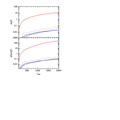
We have found that the non-Gaussian contributions $\Delta\langle\chi^{2}\rangle$, $\Delta\mbox{Var}(\chi^{2})$ to unreduced $\chi^{2}$ values are nearly independent of the number of bands or degrees of freedom. In Figure 16, we show these contributions for lensed $TT$, $EE$ and $BB$ power spectra, and for varying $l_{\rm max}$, in two extreme cases: a “many-band” fit with $\Delta l=10$, and a “one-band” fit across all multipoles up to $l_{\rm max}$. The non-Gaussian contributions are always negligible for $TT$ and $EE$; for $BB$ they are significant if the number of bands is small and $l_{\rm max}$ is sufficiently large, but can be hidden if the fit is performed using many bands. This is consistent with the discussion in §II; non-Gaussianity is hidden when considering narrow $l$ bands, but appears as extra variance when estimated $BB$ power is averaged over a wide range in $l$.

In Figure 16, we have computed $\Delta\langle\chi^{2}\rangle$ using Eq. (50), and $\Delta\mbox{Var}(\chi^{2})$ using the approximation of Eq. (51). To check this approximation, and the approximation that ${\mathcal{N}}_{ij}$ can be computed to lowest order in $C_{l}^{\phi\phi}$, we have also computed $\langle\chi^{2}\rangle$, $\mbox{Var}(\chi^{2})$ using Monte Carlo simulations of the lensed CMB, and find excellent agreement throughout Figure 16.

Appendix B Fiducial Model Dependence

Throughout this paper, we have presented results for the fiducial model of Eq. (23) which has a low ionization optical depth and correspondingly a low $\sigma_{8}=0.73$. For small deviations around the fiducial model, we have found that the shape of the principal components (Fig. 2) is unchanged, but the translation between the noise level and uncertainties $\sigma(\Theta_{i})$ in the lensing observables (Fig. 5) can be affected. Denoting the uncertainty at noise level $\Delta_{P}$ by $\sigma(\Theta_{i};\Delta_{P})$, we find the following rough scaling, expected from signal-to-noise considerations assuming that the unlensed CMB is fixed:

$$\sigma(\Theta_{1};\Delta_{P}) \approx \left(\frac{C_{l_{K1}}^{\phi\phi}}{C_{l_{K1},{\rm fid}}^{\phi\phi}}\right)\sigma_{\rm fid}(\Theta_{1};\Delta_{P})\,,$$ (52)

$$\sigma(\Theta_{2};\Delta_{P}) \approx \sigma_{\rm fid}\left[\Theta_{2};\left(\frac{C_{l_{K2}}^{\phi\phi}}{C_{l_{K2},{\rm fid}}^{\phi\phi}}\right)^{-1/2}\!\!\!\!\!\!\!\!\Delta_{P}\right]\,.$$

Here, $l_{K1}=114$, $l_{K2}=440$ are the median multipoles from §IV.1. The scaling for $\Theta_{1}$ follows from considering the unlensed CMB as a fixed noise source whereas for $\Theta_{2}$ it follows from direct signal-to-noise scaling.

The optimal noise level from Eq. (47) for measuring lensing $B$-modes scales roughly as $(C_{l_{K2}}^{\phi\phi}/C_{l_{K2},{\rm fid}}^{\phi\phi})^{1/2}$ for the same reason.

References

- Challinor and Lewis (2005) A. Challinor and A. Lewis, Phys. Rev. D71, 103010 (2005), eprint astro-ph/0502425.
- Bernardeau (1998) F. Bernardeau, Astron. Astrophys. 338, 375 (1998).
- Zaldarriaga and Seljak (1999) M. Zaldarriaga and U. Seljak, Phys. Rev. D 59, 123507 (1999), eprint astro-ph/9810257.
- Hu (2001a) W. Hu, Astrophys. J. Lett. 557, L79 (2001a), eprint astro-ph/0105424.
- Hu and Okamoto (2002) W. Hu and T. Okamoto, Astrophys. J. 574, 566 (2002), eprint astro-ph/0111606.
- Hirata and Seljak (2003) C. M. Hirata and U. Seljak, Phys. Rev. D67, 043001 (2003), eprint astro-ph/0209489.
- Hu (2001b) W. Hu, Phys. Rev. D 64, 083005 (2001b), eprint astro-ph/0105117.
- Cooray (2002) A. Cooray, Phys. Rev. D65, 063512 (2002), eprint astro-ph/0110415.
- Smith et al. (2004) K. M. Smith, W. Hu, and M. Kaplinghat, Phys. Rev. D 70, 043002 (2004), eprint astro-ph/0402442.
- Hu (2002) W. Hu, Phys. Rev. D 65, 023003 (2002), eprint astro-ph/0108090.
- Kaplinghat (2003) M. Kaplinghat, New Astronomy Review 47, 893 (2003), eprint astro-ph/0307538.
- Acquaviva and Baccigalupi (2005) V. Acquaviva and C. Baccigalupi (2005), eprint astro-ph/0507644.
- Kaplinghat et al. (2003a) M. Kaplinghat, L. Knox, and Y.-S. Song, Phys. Rev. Lett. 91, 241301 (2003a), eprint astro-ph/0303344.
- Hu (2000) W. Hu, Phys. Rev. D 62, 043007 (2000), eprint astro-ph/0001303.
- Zaldarriaga and Seljak (1998) M. Zaldarriaga and U. Seljak, Phys. Rev. D 58, 023003 (1998), eprint astro-ph/9803150.
- Spergel et al. (2006) D. N. Spergel et al. (2006), eprint astro-ph/0603449.
- Eisenstein et al. (1999) D. J. Eisenstein, W. Hu, and M. Tegmark, Astrophys. J. 518, 2 (1999), eprint astro-ph/9807130.
- Perotto et al. (2006) L. Perotto, J. Lesgourgues, S. Hannestad, H. Tu, and Y. Y. Y. Wong (2006), eprint astro-ph/0606227.
- Hu (2005) W. Hu, ASP Conf. Series 339, 215 (2005), eprint astro-ph/0407158.
- Hu and White (1996) W. Hu and M. White, Astrophys. J. 471, 30 (1996), eprint astro-ph/9602019.
- Hu et al. (2006) W. Hu, D. Huterer, and K. M. Smith, Astrophys. J. Lett. submitted (2006), eprint astro-ph/0607316.
- Knox (2006) L. Knox, Phys. Rev. D73, 023503 (2006), eprint astro-ph/0503405.
- Kaplinghat et al. (2003b) M. Kaplinghat et al., Astrophys. J. 583, 24 (2003b), eprint astro-ph/0207591.
- Holder et al. (2003) G. Holder, Z. Haiman, M. Kaplinghat, and L. Knox, Astrophys. J. 595, 13 (2003), eprint astro-ph/0302404.
- Hu and Holder (2003) W. Hu and G. P. Holder, Phys. Rev. D 68, 023001 (2003), eprint astro-ph/0303400.
- Knox and Song (2002) L. Knox and Y.-S. Song, Phys. Rev. Lett. 89, 011303 (2002), eprint astro-ph/0202286.
- Kesden et al. (2002) M. Kesden, A. Cooray, and M. Kamionkowski, Phys. Rev. Lett. 89, 1304 (2002).
- Seljak and Hirata (2004) U. Seljak and C. M. Hirata, Phys. Rev. D69, 043005 (2004), eprint astro-ph/0310163.
- Spergel et al. (2003) D. N. Spergel et al. (WMAP), Astrophys. J. Suppl. 148, 175 (2003), eprint astro-ph/0302209.