Systematic Errors in Cosmic Microwave Background Interferometry

Abstract

Cosmic microwave background (CMB) polarization observations will require superb control of systematic errors in order to achieve their full scientific potential, particularly in the case of attempts to detect the $B$ modes that may provide a window on inflation. Interferometry may be a promising way to achieve these goals. This paper presents a formalism for characterizing the effects of a variety of systematic errors on interferometric CMB polarization observations, with particular emphasis on estimates of the $B$-mode power spectrum. The most severe errors are those that couple the temperature anisotropy signal to polarization; such errors include cross-talk within detectors, misalignment of polarizers, and cross-polarization. In a $B$ mode experiment, the next most serious category of errors are those that mix $E$ and $B$ modes, such as gain fluctuations, pointing errors, and beam shape errors. The paper also indicates which sources of error may cause circular polarization (e.g., from foregrounds) to contaminate the cosmologically interesting linear polarization channels, and conversely whether monitoring of the circular polarization channels may yield useful information about the errors themselves. For all the sources of error considered, estimates of the level of control that will be required for both $E$ and $B$ mode experiments are provided. Both experiments that interfere linear polarizations and those that interfere circular polarizations are considered. The fact that circular experiments simultaneously measure both linear polarization Stokes parameters in each baseline mitigates some sources of error.

I Introduction

Cosmic microwave background (CMB) polarimetry is one of the most exciting frontiers in cosmology. CMB polarization has already been detected Kovac et al. (2002); Kogut et al. (2003); Readhead et al. (2004); Leitch et al. (2005); Barkats et al. (2005); Page et al. (2006), and we may expect future instruments to characterize the polarization signal in much greater detail (e.g., Korotkov et al. (2006)). In the near future, CMB polarization data are expected to refine estimates of cosmological parameters Kinney (1998), probe the ionization history of the Universe Zaldarriaga (1997) and the details of recombination Peebles et al. (2000), and measure gravitational lensing due to large-scale structure Zaldarriaga and Seljak (1998). Most exciting of all, polarization maps may provide a direct probe of an inflationary epoch in the extremely early Universe by detecting the signature of primordial gravitational radiation Zaldarriaga and Seljak (1997); Seljak and Zaldarriaga (1997); Kamionkowski et al. (1997a, b).

A crucial insight into the analysis of CMB polarization data is the fact that any CMB polarization map can be divided into two components, a scalar component, traditionally denoted $E$, and a pseudoscalar component called $B$. The CMB is weakly polarized, meaning that both of these components are much smaller than the unpolarized (temperature) anisotropy. Furthermore, the $B$ component is expected to be much weaker than $E$, since scalar density perturbations produce only $E$ to linear order Zaldarriaga and Seljak (1997); Seljak and Zaldarriaga (1997); Kamionkowski et al. (1997a, b). (See Figure 1.) Experiments to date have detected only the $E$ component. In the future, the search for the weaker $B$-type polarization will be a high priority, as the $B$ modes may contain the imprint of gravitational waves produced during inflation.

Figure 1: Power spectra for temperature anisotropy (T), $TE$ cross-correlation (X, absolute value plotted), $E$-type polarization, and $B$-type polarization. The best-fit parameters from the three-year WMAP data were used Spergel et al. (2006) with a tensor-to-scalar ratio $T/S=0.01$. The right panel shows the ratios of the power spectra.

Characterization of CMB polarization requires both very low noise and exquisite control of systematic errors. In particular, some sources of systematic error may cause the polarization signal to be contaminated by the much larger unpolarized anisotropy, while others mix the $E$ and $B$ components. As efforts to design $B$-mode experiments intensify, it is important to consider carefully the susceptibility of different designs to various kinds of error. Hu et al. Hu et al. (2003) have provided a detailed framework for performing such an analysis in the context of an imaging experiment. For interferometric measurements, the issues are somewhat different. The purpose of this paper is to forecast the effects of a variety of systematic errors on interferometric measurements.

Interferometric methods have played an important role in measurements of CMB anisotropy and polarization. Pioneering attempts to detect CMB anisotropy with interferometers are described in Martin and Partridge (1988) and Subrahmanyan et al. (1993). Several groups have successfully detected primary CMB anisotropies (O’Sullivan et al., 1995; Baker et al., 1999; Halverson et al., 2002; Pearson et al., 2003; Taylor et al., 2003) and polarization (Readhead et al., 2004; Leitch et al., 2005) using interferometers. The formalism for analyzing CMB data from interferometers has been developed by a number of authors Hobson et al. (1995); Hobson and Magueijo (1996); White et al. (1999); Hobson and Maisinger (2002); Myers et al. (2003); Bunn and White (2006) as well as in the experimental papers cited above.

In any data set that fails to cover the entire sky, it is impossible to separate the $E$ and $B$ components perfectly Lewis et al. (2002); Bunn (2002a, b); Bunn et al. (2003). The operation of separating a polarization map into $E$ and $B$ components is nonlocal when the map is viewed in real space, but in Fourier space or spherical harmonic space, it can be done locally (mode by mode). Since interferometric data sample the sky in the Fourier domain, $E$-$B$ separation may be cleaner for interferometric data than for maps made with single-dish instruments Park et al. (2003); Park and Ng (2004).

As we will see, a variety of systematic errors in interferometers can be modeled via Jones matrices Tinbergen (1996); Heiles et al. (2001); Hu et al. (2003) and by deviations of the antenna patterns (including cross-polar contributions) from assumed ideal forms. We will assume that each of these errors can be characterized by small unknown parameters, such as gain fluctuations, cross-talk between detectors, pointing errors, etc. We will first calculate the effect of each error on the measured visibilities. We will then provide a method of quantifying the effects of each of these errors on estimates of the polarization power spectra $C_{l}^{E},C_{l}^{B}$ that can be obtained from a hypothetical data set.

This paper has the following structure. Section II presents the mathematical formalism we will use to describe interferometric visibilities for polarization data. Section III presents the effects of various systematic errors on the visibilities extracted from a hypothetical CMB experiment. Section IV presents a method of forecasting errors on power spectrum estimates from errors on visibilities. Sections V and VI contain results showing how the error forecasts on both $E$ and $B$ power spectra depend on the parameters that characterize the various systematic errors. Section VII presents a discussion of the implications of these results, and a brief appendix contains a useful mathematical result.

Sections IV through VI contain quite a bit of technical detail. The particularly busy or impatient reader should note that the key ideas of Section IV are summarized at the beginning, and the final results of Sections V and VI are summarized in Section VII and Table 1.

II Formalism

II.1 Antenna Patterns

Consider a monochromatic plane wave of angular frequency $\omega=2\pi c/\lambda$ approaching the origin from a direction $\hat{\bf r}$. The electric field of the wave is

$${\bf E}({\bf x},t;\hat{\bf r})={\bm{\epsilon}_{\rm in}}(\hat{\bf r})e^{i({\bf k}\cdot{\bf x}-\omega t)},$$ (1)

where the wave vector ${\bf k}=-(\omega/c)\hat{\bf r}$. (Of course, as usual the physical electric field is just the real part of this complex quantity.)

The complex vector ${\bm{\epsilon}_{\rm in}}(\hat{\bf r})$ is perpendicular to $\hat{\bf r}$. Its direction fluctuates rapidly in time (except in the case of completely polarized radiation). As usual, all observables will be averages taken over a time that is long compared to those fluctuations. To be specific, let $({\epsilon_{\rm in}}_{X},{\epsilon_{\rm in}}_{Y})$ be Cartesian components of ${\bm{\epsilon}_{\rm in}}$ in the plane perpendicular to $\hat{\bf r}$, and define a $2\times 2$ matrix ${\bf S}$ with components

$$S_{ij}\propto\langle E_{i}E_{j}^{*}\rangle=\langle{\epsilon_{\rm in}}_{i}{{\epsilon}_{\rm in}^{*}}_{j}\rangle,$$ (2)

where $i,j$ range over $X,Y$. The matrix ${\bf S}$ can be expressed in terms of the standard Stokes parameters

$${\bf S}=\begin{pmatrix}I+Q&U+iV\\ U-iV&I-Q\end{pmatrix}.$$ (3)

The constant of proportionality in equation (2) depends on the system of units being used. We will follow the common practice in CMB studies of expressing all Stokes parameters in dimensionless “$\Delta T/T$” form.

In general the electric field at any given point will be a superposition of waves coming in from all directions $\hat{\bf r}$. We assume that the temporal fluctuations in the incoming waves from two distinct directions are uncorrelated with each other:

$$\langle{\epsilon_{\rm in}}_{i}(\hat{\bf r}_{1}){\epsilon_{\rm in}}_{j}(\hat{\bf r}_{2})^{*}\rangle=S_{ij}(\hat{\bf r}_{1})\delta(\hat{\bf r}_{1}-\hat{\bf r}_{2}),$$ (4)

with $S_{ij}$ related to the Stokes parameters as above.

Consider a single-mode antenna that is designed to be sensitive to only one polarization direction. We can model this antenna as a device that sums all of the incoming radiation, weighted by some vector-valued antenna pattern ${\bf a}$, to produce an output that is the real part of

$${\epsilon_{\rm out}}=\int d^{2}\hat{\bf r}\,{\bf a}(\hat{\bf r})\cdot{\bm{\epsilon}_{\rm in}}(\hat{\bf r})e^{i({\bf k}\cdot{\bm{\xi}}-\omega t)},$$ (5)

where ${\bm{\xi}}$ is the location of the antenna.

Throughout this paper, we will consider experiments in which the beam width is small enough that the flat-sky approximation is appropriate in analyzing any single pointing of the instrument. (Mosaicking of multiple pointings of such an instrument is considered in Bunn and White (2006).) In that case, we can represent the direction $\hat{\bf r}$ by a vector in the plane (specifically, the tangent plane to the sphere at the pointing center) with components $(x,y)$. In this approximation, for instance, an antenna with a Gaussian beam pattern that is sensitive only to linear polarization the $\hat{\bf x}$ direction would have ${\bf a}\propto\hat{\bf x}\exp[-(x^{2}+y^{2})/(4\sigma^{2})]$, while an antenna that is sensitive to either right or left circular polarization would have $\hat{\bf x}\pm i\hat{\bf y}$ in place of $\hat{\bf x}$. The factor 4 in the Gaussian is present because we would like $\sigma$ to be the Gaussian width of $|{\bf a}|^{2}$, not ${\bf a}$.

In some experiments, the same antenna may be used to measure two polarization states (typically either “horizontal” and “vertical” linear polarization, or left and right circular polarization). In that case, the output of the antenna will be a two-component vector ${\bm{\epsilon}_{\rm out}}$, and the antenna pattern will be a $2\times 2$ matrix ${\bf A}$:

$${\bm{\epsilon}_{\rm out}}=\int d^{2}\hat{\bf r}\,{\bf A}(\hat{\bf r})\cdot{\bm{\epsilon}_{\rm in}}(\hat{\bf r})e^{i({\bf k}\cdot{\bm{\xi}}-\omega t)}.$$ (6)

In general, we will model antennas as sensitive to two polarization states in this manner. If in a particular experiment only one output is actually measured, we can simply ignore the other component of ${\bm{\epsilon}_{\rm out}}$.

We can of course express the components of the vectors ${\bm{\epsilon}_{\rm in}}$ and ${\bm{\epsilon}_{\rm out}}$ in any basis we like. In particular, we can resolve these vectors in either a linear polarization basis with components $(\epsilon_{X},\epsilon_{Y})$ or a right- and left-circular basis with components $(\epsilon_{R},\epsilon_{L})$. The two bases are related by a unitary transformation

$$\begin{pmatrix}\epsilon_{R}\\ \epsilon_{L}\end{pmatrix}={\bf R}_{\rm circ}\cdot\begin{pmatrix}\epsilon_{x}\\ \epsilon_{y}\end{pmatrix},$$ (7)

with

$${\bf R}_{\rm circ}=\frac{1}{\sqrt{2}}\begin{pmatrix}1&i\\ 1&-i\end{pmatrix}.$$ (8)

In either case, an ideal antenna, i.e., one with equal response to both polarization states and no mixing between them, would have ${\bf A}$ equal to a scalar function times the identity matrix.

In the circular polarization basis, the elements of the Stokes parameter matrix ${\bf S}$ become

$${\bf S}_{\rm circ}={\bf R}_{\rm circ}\cdot{\bf S}_{\rm lin}\cdot{\bf R}_{\rm circ}^{-1}$$ (9)

with ${\bf S}_{\rm lin}$ given by equation (3). Explicitly, we have

$${\bf S}_{\rm circ}=\begin{pmatrix}I+V&Q+iU\\ Q-iU&I-V\end{pmatrix}.$$ (10)

II.2 Visibilities

Consider an interferometer with $N$ antennas. The output signal from antenna $j$ will be denoted ${\bm{\epsilon}_{\rm out}^{(j)}}$. As noted earlier, we will treat this as a two-component vector with components ${{\epsilon}_{\rm out}^{(j)}}_{m}$, with $m=X,Y$ for a linear polarization experiment or $m=R,L$ for a circular polarization experiment.

The basic datum for an interferometer is a “visibility” obtained by correlating a component of ${\epsilon_{\rm out}}$ from one antenna with a component from another antenna:

$$V_{mn}^{(jk)}=\langle{{\epsilon}_{\rm out}^{(j)}}_{m}{{\epsilon}_{\rm out}^{(k)*}}_{\!\!n}\rangle,$$ (11)

where the angle brackets denote a time average. Both real and imaginary parts of this complex quantity can be obtained by measuring the in-phase and quadrature-phase correlations.

For a fixed pair of antennas $(jk)$, the visibilities form a $2\times 2$ matrix ${\bf V}^{(jk)}$. Using equations (4) and (6), we can write this matrix as

$${\bf V}^{(jk)}=\int d^{2}\hat{\bf r}\,{\bf A}^{(j)}(\hat{\bf r})\cdot{\bf S}(\hat{\bf r})\cdot{\bf A}^{(k){\dagger}}(\hat{\bf r})\ e^{-2\pi i{\bf u}_{jk}\cdot\hat{\bf r}}.$$ (12)

Here the ${\bf A}$’s are the antenna patterns for the two antennas and ${\bf u}_{jk}=(\bm{\xi}^{(k)}-\bm{\xi}^{(j)})/\lambda$ is the separation between the two antennas in units of wavelength. The matrix ${\bf A}^{\dagger}$ is the hermitian conjugate of ${\bf A}$ (that is, the complex conjugate of the transpose of ${\bf A}$).

In an ideal experiment with ${\bf A}$ proportional to the identity matrix (no cross-polar response and identical co-polar response to both polarization states), ${\bf V}^{(jk)}\propto{\bf S}$. In other words, each visibility measures a simple linear combination of the Stokes parameters. To be explicit, let us define Stokes visibilities

$$V_{Z}^{(jk)}\equiv\int d^{2}\hat{\bf r}\,A^{(j)}(\hat{\bf r})Z(\hat{\bf r})A^{(k)}(\hat{\bf r})e^{-2\pi i{\bf u}_{jk}\cdot\hat{\bf r}},$$ (13)

where $Z=I,Q,U,V$ is a Stokes parameter. As is well known, these can also be written as a convolution in Fourier space:

$$V_{Z}^{(jk)}\propto\int d^{2}{\bf k}\,\tilde{Z}({\bf k})\widetilde{\cal A}_{jk}^{*}({\bf k}-2\pi{\bf u})$$ (14)

with ${\cal A}_{jk}=A^{(j)}A^{(k)}$.

A polarimetric interferometer can work either by interfering linear polarization states or circular polarization states. Throughout this paper, we will refer to these possibilities as linear experiments and circular experiments respectively. Information about both linear and circular polarization can be obtained from either type of experiment.

In an ideal linear experiment, we would extract the Stokes parameters from the visibility matrix as follows:

$$V_{I} =\tfrac{1}{2}(V_{XX}+V_{YY}),$$ (15a)

$$V_{Q} =\tfrac{1}{2}(V_{XX}-V_{YY}),$$ (15b)

$$V_{U} =\tfrac{1}{2}(V_{XY}+V_{YX}),$$ (15c)

$$V_{V} =\tfrac{1}{2i}(V_{XY}-V_{YX}).$$ (15d)

Here we are assuming that all antennas split up the incoming radiation into orthogonal linear polarizations with respect to a single fixed coordinate system $(X,Y)$. The superscript $(jk)$ is suppressed.

For the weak polarization found in CMB data, equation (15b) is not a practical way to measure Stokes $Q$ because it requires perfect cancellation of the much larger $I$ contributions; in practice, such an experiment measures linear polarization only via $U$, not $Q$. Since $Q\to U$ under a $45^{\circ}$ rotation, we measure $Q$ in practice by using antennas that measure linear polarization states in a basis $(X^{\prime},Y^{\prime})$ that is rotated with respect to $(X,Y)$. This can be done either by rotating the instrument or by having the polarizers on different antennas oriented in different ways. In either case, note that in general the Stokes parameters $Q,U$ are not generally measured with the same baseline at the same time.

The corresponding relations in a circular experiment are

$$V_{I} =\tfrac{1}{2}(V_{RR}+V_{LL}),$$ (16a)

$$V_{Q} =\tfrac{1}{2}(V_{RL}+V_{LR}),$$ (16b)

$$V_{U} =\tfrac{1}{2i}(V_{RL}-V_{LR}),$$ (16c)

$$V_{V} =\tfrac{1}{2}(V_{RR}-V_{LL}).$$ (16d)

In a circular experiment, both $Q$ and $U$ visibilities can be measured simultaneously on a single baseline.

We do not expect any cosmological source of circular polarization: Stokes $V$ is expected to be zero. Nonetheless, it may be useful to measure the Stokes visibility $V_{V}$ as a monitor of systematic errors. Conversely, if a non-cosmological source of circular polarization is present, systematic errors may cause it to contribute to measurements of linear polarization.

II.3 Modeling systematic errors

A wide variety of systematic errors can be modeled as imperfections in the matrix-valued antenna patterns of the antennas. We will model these errors in the following way:

$${\bf A}(\hat{\bf r})={\bf J}_{i}\cdot{\bf R}\cdot{\bf A}_{s}(\hat{\bf r})\cdot{\bf R}^{-1}.$$ (17)

Here ${\bf R}$ is ${\bf R}_{\rm circ}$ for a circular experiment and is the identity matrix for a linear experiment.

The “instrument Jones matrix” ${\bf J}_{i}$ represents errors introduced within the instrument, such as gain errors and cross-talk between the two outputs of a given antenna. The matrix ${\bf A}_{s}$ is the antenna pattern on the sky, before such instrumental errors are taken into account. We use ${\bf A}_{s}$ to model cross-polarization, beam errors, pointing errors, etc. We will always use ${\bf A}$ (with no subscript) to denote the overall antenna pattern including both “instrument” and “sky” effects.

We will always represent ${\bf A}_{s}$ in a Cartesian basis; that is, it acts on components $({\epsilon_{\rm in}}_{X},{\epsilon_{\rm in}}_{Y})$. When we are performing a circular experiment, however, ${\bm{\epsilon}_{\rm in}}$ and ${\bm{\epsilon}_{\rm out}}$ will be represented in a circular polarization basis. The factors ${\bf R}$ and ${\bf R}^{-1}$ are inserted to account for this change of basis.

An ideal instrument would have ${\bf J}_{i}={\bf 1}$, the identity matrix, and ${\bf A}_{s}=A(\theta,\phi){\bf 1}$.

There is some redundancy in equation (17). Mathematically, we could correctly describe any instrument without including ${\bf J}_{i}$ by simply absorbing its effects into ${\bf A}_{s}$. However, it is convenient to maintain the distinction between effects that happen to the signal before the antenna averages over the beam (effects “on the sky”) and afterwards (effects “in the instrument”). Instrument errors are easier to model, because by definition they do not depend on position on the sky.

III Effect of errors on visibilities

In this section we compute the effects of various sorts of instrument and beam errors on the measured visibilities $V_{Q},V_{U}$. Each of the errors considered can be modeled with a set of small parameters. We assume that the experimenter has no knowledge of these errors (or else she would have removed them) and hence analyzes the data under the assumption that the experiment is error-free.

III.1 Instrument Errors

Consider first the effect of errors within the instrument, assuming for the moment that ${\bf A}_{s}$ is of the ideal form $A_{s}(\hat{\bf r}){\bf 1}$. We can completely characterize the instrumental Jones matrix for the $j$th antenna with gain errors $g_{1}^{(j)},g_{2}^{(j)}$ and couplings $\epsilon_{1}^{(j)},\epsilon_{2}^{(j)}$:

$${\bf J}_{i}^{(j)}=\begin{pmatrix}1+g_{1}^{(j)}&\epsilon_{1}^{(j)}\\ \epsilon_{2}^{(j)}&1+g_{2}^{(j)}\end{pmatrix}.$$ (18)

This is similar to the characterization in ref. Hu et al. (2003), although our notation is not identical to theirs. In particular, we treat the $g$ and $\epsilon$ parameters as complex numbers (to account for arbitrary phases in the errors) rather than introducing explicit phase angles. The parameters $g$ and $\epsilon$ will be assumed to be small (i.e., products of them will be neglected).

A number of different physical effects can be encoded in a matrix of this form. The gain parameters $g_{i}^{(j)}$ incorporate both errors in the magnitude of the gain and unaccounted-for phase delays. The couplings $\epsilon_{i}^{(j)}$ can account for mixing of the two polarization states within the optical and electronic systems and also, in the case of a linear experiment, for an error in alignment of the polarizers: if the polarizers in antenna $j$ are misaligned by an angle $\delta$, then $\epsilon_{1}^{(j)}=\delta$, $\epsilon_{2}^{(j)}=-\delta$.

By using this model for the antenna patterns in equation (12), we can determine the effect of all of these errors on the recovered Stokes visibilities. The results depend on whether we are considering a linear or circular experiment.

Linear experiment: Information about linear polarization in such an experiment comes from the visibility for Stokes $U$. Using equations (3), (12), and (15c), we find

$$V_{U}^{(jk)}=\accentset{\circ}{V}_{U}^{(jk)} +\frac{1}{2}\left[\accentset{\circ}{V}_{I}^{(jk)}(\epsilon_{1}^{(j)}+\epsilon_{2}^{(j)}+\epsilon_{1}^{(k)*}+\epsilon_{2}^{(k)*})\right.$$

$$+\accentset{\circ}{V}_{U}^{(jk)}(g_{1}^{(j)}+g_{2}^{(j)}+g_{1}^{(k)*}+g_{2}^{(k)*})$$

$$+\accentset{\circ}{V}_{Q}(-\epsilon_{1}^{(j)}+\epsilon_{2}^{(j)}-\epsilon_{1}^{(k)*}+\epsilon_{2}^{(k)*})$$

$$+\left.\accentset{\circ}{V}_{V}(g_{1}^{(j)}-g_{2}^{(j)}-g_{1}^{(k)*}+g_{2}^{(k)*})\right],$$ (19)

working to linear order in the small quantities. Here the symbol $\accentset{\circ}{V}$ indicates the visibility that would be measured in the absence of systematic errors. Note that the coupling parameters $\epsilon$ mix temperature anisotropy ($I$) into polarization; this is in general the most serious sort of error. The $\accentset{\circ}{V}_{Q}$ and $\accentset{\circ}{V}_{U}$ terms are less worrisome, since they only involve polarization. However, as we will see they do couple $E$ to $B$ and so can be serious for a $B$-mode experiment.

Although for cosmological purposes we are primarily interested in measurements of linear polarization, with this experimental setup we get the visibility for Stokes $V$ “for free” by subtracting rather than adding $V_{XY}$ and $V_{YX}$ [see equations (15)]. Assuming there is no intrinsic circular polarization ($\accentset{\circ}{V}_{V}=0$), the leading contribution is

$$V_{V}^{(jk)}=\frac{i}{2}\accentset{\circ}{V}_{I}^{(jk)}(\epsilon_{1}^{(j)}-\epsilon_{2}^{(j)}-\epsilon_{1}^{(k)*}+\epsilon_{2}^{(k)*}),$$ (20)

neglecting terms proportional to $\accentset{\circ}{V}_{Q},\accentset{\circ}{V}_{U}$. Even very low levels of coupling may therefore provide a measurable signal, which would be correlated in a known way with the temperature map. This may provide a useful diagnostic.

Conversely, if there is intrinsic circular polarization (e.g., due to foregrounds, equation (19) shows that gain errors can couple that signal into $V_{Q},V_{U}$.

Circular experiment: Now suppose we perform an experiment in which interference between right and left circular polarization states is measured. Using equations (10), (12), (16b) and (16c), we find

$$V_{Q}^{(jk)}= \accentset{\circ}{V}_{Q}^{(jk)}+\frac{1}{2}\left[\accentset{\circ}{V}_{I}^{(jk)}(\epsilon_{1}^{(j)}+\epsilon_{2}^{(j)}+\epsilon_{1}^{(k)*}+\epsilon_{2}^{(k)*})\right.$$

$$+\accentset{\circ}{V}_{Q}^{(jk)}(g_{1}^{(j)}+g_{2}^{(j)}+g_{1}^{(k)*}+g_{2}^{(k)*})$$

$$+i\accentset{\circ}{V}_{U}^{(jk)}(g_{1}^{(j)}-g_{2}^{(j)}-g_{1}^{(k)*}+g_{2}^{(k)*})$$

$$+\left.\accentset{\circ}{V}_{V}^{(jk)}(-\epsilon_{1}^{(j)}+\epsilon_{2}^{(j)}-\epsilon_{1}^{(k)*}+\epsilon_{2}^{(k)*})\right],$$ (21a)

$$V_{U}^{(jk)}= \accentset{\circ}{V}_{U}^{(jk)}+\frac{1}{2}\left[i\accentset{\circ}{V}_{I}^{(jk)}(-\epsilon_{1}^{(j)}+\epsilon_{2}^{(j)}+\epsilon_{1}^{(k)*}-\epsilon_{2}^{(k)*})\right.$$

$$+\accentset{\circ}{V}_{U}^{(jk)}(g_{1}^{(j)}+g_{2}^{(j)}+g_{1}^{(k)*}+g_{2}^{(k)*})$$

$$-i\accentset{\circ}{V}_{Q}^{(jk)}(g_{1}^{(j)}-g_{2}^{(j)}-g_{1}^{(k)*}+g_{2}^{(k)*})$$

$$+\left.i\accentset{\circ}{V}_{V}^{(jk)}(\epsilon_{1}^{(j)}+\epsilon_{2}^{(j)}-\epsilon_{1}^{(k)*}-\epsilon_{2}^{(k)*})\right].$$ (21b)

As in the linear case, coupling errors ($\epsilon$) are the main danger, causing leakage from $I$ into $Q,U$. Gain errors mix $V_{Q}$ and $V_{U}$ with each other. As we will see, this means that their effect on the $B$ mode power spectrum is somewhat more severe than in the case of a linear experiment.

As for linear experiments, we might consider monitoring the circular polarization visibility $V_{V}$ as a diagnostic, even though we do not expect any cosmological signal. In this case, the leading term in $V_{V}$ is proportional to the gain fluctuations $g_{i}^{(j)}$ and to $\accentset{\circ}{V}_{I}$. Since gain errors are less worrisome than couplings, this may not be as valuable as in the linear case. Furthermore, unlike a linear experiment, in a circular experiment one does not necessarily get $V_{V}$ for free when measuring $V_{Q},V_{U}$: the linear polarization information is obtained by interfering right with left polarization states, while $V_{V}$ comes from interfering identical ones [see equation (16)].

III.2 Beam Errors

We next consider errors that can be modeled via the “sky” matrix ${\bf A}_{s}$. In this section we ignore instrument errors, taking ${\bf J}_{i}$ to be the identity matrix.

An ideal experiment, with ${\bf A}_{s}$ equal to a scalar function times the identity matrix, would have identical response to both polarization states and no mixing between them. Furthermore, ideally ${\bf A}_{s}$ would be the same for all antennas. There are of course a large number of ways these idealizations can fail. Unlike instrument errors, which are characterized by a finite list of parameters, beam errors are characterized by arbitrary functions on the sky. Rather than providing a complete catalogue of this infinite space of possibilities, we focus on a few physically motivated possibilities.

Beam mismatch: We first consider the case where each antenna pattern is proportional to the identity matrix, but the various antenna patterns differ from each other and from the form assumed by the experimenter:

$${\bf A}_{s}^{(j)}(\hat{\bf r})=A^{(j)}(\hat{\bf r}){\bf 1}.$$ (22)

In this case, we are assuming no cross-polar response and identical beam patterns for both polarizations in each antenna. This formulation can account for pointing errors as well as errors in beam shape (e.g., beam width and ellipticity errors).

Assuming this form for the antenna pattern, we can use equation (12) to extract the Stokes visibilities, yielding

$$V_{Z}^{(jk)}=\int d^{2}\hat{\bf r}\,e^{-2\pi i{\bf u}_{jk}\cdot\hat{\bf r}}Z(\hat{\bf r})A^{(j)}(\hat{\bf r})A^{(k)*}(\hat{\bf r}).$$ (23)

For $Z=\{I,Q,U,V\}$. These results apply to both linear and circular experiments, although in practice only $V_{U}$ would be used for linear polarization information in a linear experiment.

This category of error causes no leakage from $I$ into polarization or even between $Q$ and $U$. Nonetheless, as we will see it can cause $E/B$ mixing when the power spectra are estimated.

Cross-polarization: We now consider the possibility of cross-polar antenna response (i.e., off-diagonal entries in ${\bf A}_{s}$). For simplicity, we consider only the case of an azimuthally symmetric antenna. We therefore begin by determining what form of ${\bf A}_{s}$ are compatible with azimuthal symmetry.

First, note that ${\bf A}_{s}$ must be diagonal when measured along the $x$ axis of our coordinate system. One way to see this is to invoke reflection symmetry: if ${\epsilon_{\rm in}}_{x}$ coupled to ${\epsilon_{\rm out}}_{y}$ along the $x$ axis, the coupling would have to change sign upon reflection, but a symmetric antenna should be invariant under reflections. Using polar coordinates $(r,\phi)$, we can therefore write

$${\bf A}^{(i)}_{s}(r,0)=\begin{pmatrix}A^{(i)}_{0}(r)+\frac{1}{2}A^{(i)}_{1}(r)&0\\ 0&A^{(i)}_{0}(r)-\frac{1}{2}A^{(i)}_{1}(r)\end{pmatrix}$$ (24)

for arbitrary radial functions $A^{(i)}_{0},A^{(i)}_{1}$. Suppose we now measure the antenna pattern for some nonzero $\phi$. We must get the same answer as at $\phi=0$, as long as we transform both ${\bm{\epsilon}_{\rm in}}$ and ${\bm{\epsilon}_{\rm out}}$ by a rotating through an angle $-\phi$ to move them to the $x$ axis. We conclude that ${\bf A}_{s}(r,\phi)={\bf R}_{-\phi}\cdot{\bf A}_{s}(r,0)\cdot{\bf R}_{\phi}$, where ${\bf R}_{\pm\phi}$ are the appropriate rotation matrices. Performing the matrix multiplication, we find that

$${\bf A}_{s}^{(i)}=\begin{pmatrix}A_{0}^{(i)}+\frac{1}{2}A_{1}^{(i)}\cos 2\phi&\frac{1}{2}A_{1}^{(i)}\sin 2\phi\\ \frac{1}{2}A_{1}^{(i)}\sin 2\phi&A_{0}^{(i)}-\frac{1}{2}A_{1}^{(i)}\cos 2\phi\end{pmatrix}.$$ (25)

Assuming the form (25) for ${\bf A}_{s}$, we obtain the following expressions for the visibilities:

$$V_{Q}^{(jk)} =\int d^{2}\hat{\bf r}\,e^{-2\pi i{\bf u}_{jk}\cdot{\bf r}}\left\{Q(\hat{\bf r})A_{0}^{(j)}(r)A_{0}^{(k)*}(r)+\right.$$

$$.\tfrac{1}{2}I(\hat{\bf r})[A_{0}^{(j)}(r)A_{1}^{(k)*}(r)+A_{1}^{(j)}(r)A_{0}^{(k)*}(r)]\cos 2\phi+$$

$$\left.\tfrac{i}{2}V(\hat{\bf r})[A_{0}^{(j)}(r)A_{1}^{(k)*}(r)-A_{1}^{(j)}(r)A_{0}^{(k)*}(r)]\sin 2\phi\right\},$$ (26a)

$$V_{U}^{(jk)} =\int d^{2}\hat{\bf r}\,e^{-2\pi i{\bf u}_{jk}\cdot{\bf r}}\left\{U(\hat{\bf r})A_{0}^{(j)}(r)A_{0}^{(k)*}(r)+\right.$$

$$\tfrac{1}{2}I(\hat{\bf r})[A_{0}^{(j)}(r)A_{1}^{(k)*}(r)+A_{1}^{(j)}(r)A_{0}^{(k)*}(r)]\sin 2\phi-$$

$$\left.\tfrac{i}{2}V(\hat{\bf r})[A_{0}^{(j)}(r)A_{1}^{(k)*}(r)-A_{1}^{(j)}(r)A_{0}^{(k)*}(r)]\cos 2\phi\right\},$$ (26b)

neglecting terms that are quadratic in the small quantities $A_{1}$. Again, these results apply to both linear and circular experiments, although only $V_{U}$ is used for polarization measurements in a linear experiment. We immediately see that cross-polarization has the danger of coupling $I$ to polarization.

If we write down a similar expression for the circular polarization visibility $V_{V}$, we find terms proportional to Stokes $Q$ and $U$ but not $I$; thus no great insight into cross-polarization is likely to be found by monitoring $V_{V}$. On the other hand, if there is a strong intrinsic circular polarization signal from foregrounds, cross-polarization may cause it to contaminate the linear polarization observables.

IV Effects on Power Spectra

IV.1 Introduction

The primary goal of almost any CMB experiment is to measure some or all of the temperature and polarization power spectra. We must therefore consider how to propagate the errors described above to obtain forecasts of the effects of various systematic errors on power spectrum estimates. The completely correct approach to this question is to define a precise experimental setup and simulate it in detail. We will instead adopt an approach that is simpler and more general.

The power spectra are well-localized in Fourier or spherical harmonic space and therefore not at all localized in image space. Interferometric visibilities are fairly well-localized in Fourier space, so power spectrum estimates can be obtained from individual visibilities (or in the case of polarization, from pairs of visibilities $V_{Q},V_{U}$). This is in contrast to an imaging experiment, in which the entire map goes into each power spectrum estimate. We can therefore assess the effects of various errors on power spectrum estimates by working with one visibility pair at a time. Naturally, analysis of real data would be considerably more sophisticated than the process we consider here, but this approach is adequate for assessing the rough scale at which each systematic error affects power spectrum estimates. The rest of this section will present this approach in detail.

A data set from an interferometric experiment consists of measurements of the visibilities $V_{Q},V_{U}$ for many different baseline separations and instrument orientations – that is, for many different values of ${\bf u}$. Let us assume that our data set consists of a set of visibilities $V_{Q1},V_{U1},V_{Q2},V_{U2},\ldots,V_{QN},V_{UN}$. We will assume that $V_{Qi},V_{Ui}$ are both measured with the same baseline vector ${\bf u}_{i}$, and furthermore that distinct baselines ${\bf u}_{i},{\bf u}_{j}$ are far enough apart in the Fourier plane that we can treat the corresponding visibilities as uncorrelated: $|{\bf u}_{i}-{\bf u}_{j}|\gtrsim\Delta u$, where the Fourier-space resolution $\Delta u$ scales inversely with the beam width. In a real experiment, these assumptions would presumably not be true: at least some regions of the visibility plane would be oversampled, and in the case of a linear experiment the two Stokes parameters would not always be measured with identical baselines. In such a case, we can imagine binning the visibilities so as to consider a smaller number of effectively independent samples in the visibility plane.

In this approximation, each set of visibilities $(V_{Qi},V_{Ui})$ gives us an independent estimate of the power spectra $C_{l}^{E},C_{l}^{B}$ at $l\approx 2\pi u_{i}$. (Here “independent” means “independent of the estimates obtained from the other visibilities”; unfortunately, it is not in general the case that the estimates of $C_{l}^{E}$ and $C_{l}^{B}$ are independent of each other.) We therefore begin by assessing the effect of each systematic error on the power spectrum estimates derived from a single pair of visibilities $(V_{Q},V_{U})$ for some fixed baseline vector ${\bf u}$. We assume that systematic errors must be controlled at least well enough that the fractional errors introduced in the power spectrum estimates from each individual visibility are small.

In this section, we begin with the optimal estimators of $E$ and $B$ band powers from a single visibility pair $(V_{Q},V_{U})$ under the idealized assumption that there are no errors in the experiment. We then imagine “turning on” sources of systematic error, one at a time, and show how to calculate the resulting root-mean-square (r.m.s.) band power errors. We will find that the r.m.s. error induced by any particular systematic error can be written in the form

$$(\delta\hat{C}_{\rm rms}^{K})^{2}=p_{\rm rms}^{2}\sum_{I,J}{\kappa^{2}_{{}_{K,IJ,p}}}C^{I}C^{J}.$$ (27)

Here $p$ is a parameter characterizing the strength of the source of error, (e.g., one of the gain fluctuation parameters $g_{i}^{(j)}$). The superscript $K=\{E,B\}$ indicates the type of power spectrum being measured, and $\delta\hat{C}_{\rm rms}^{K}$ is the error in an estimate of a band power. The quantities $C^{I},C^{J}$ are band powers with $I,J$ ranging over $\{T,X,E,B\}$ (temperature, $TE$ cross-correlation, and $E$ and $B$ polarization spectra). We will see how to calculate the coefficients $\kappa$ below.

As Figure 1 shows, there is a clear hierarchy in the input power spectra: $C^{T}>C^{X}>C^{E}>C^{B}$. The above sum is therefore usually dominated by one or at most two terms that couple large spectra to smaller ones. For each of the sources of error described in the previous sections, we can find the one or two most serious such couplings and thus estimate the level to which the overall error must be controlled or at least understood.

As noted above, our approach is to demand that errors be understood to a level low enough that they do not contaminate band powers measured from each individual baseline. This may be regarded as a conservative approach: even if an error has quite a large effect on power spectrum estimates from a single baseline, it may still be possible to extract good power spectrum estimates by combining results from a set of many baselines. This is particularly true if the visibility plane is heavily oversampled, with many different visibilities within a resolution element $\Delta u$, if the errors associated with the various visibilities are independent and average to zero. However, since systematic errors are in general non-Gaussian and time-varying, one would not want to rely on such an averaging procedure unless the statistical properties of the errors are understood quite well. It therefore seems reasonable to adopt such a conservative approach.

IV.2 Ideal estimators

We begin with the estimators for $E$ and $B$ band powers for a single visibility pair $(V_{Q},V_{U})$, for an idealized experiment with all systematic errors “turned off.” In the following subsection, we will examine the effect on these estimators when the errors are introduced.

Let ${\bf v}\equiv(V_{I},V_{Q},V_{U})$ be a set of visibilities corresponding to a single baseline ${\bf u}$. Our hypothetical experiment measures $V_{Q}$ and $V_{U}$, but not necessarily $V_{I}$. As we will see, it is convenient to include $V_{I}$ in the formalism anyway, because it may be coupled to the others by various systematic errors.

In the absence of systematic errors, the $I$ visibility measures only the temperature fluctuations:

$$\langle|V_{I}|^{2}\rangle=C^{T}_{2\pi u}.$$ (28)

Here $C_{2\pi u}^{T}$ is a band power giving the average temperature power spectrum in the vicinity of $l=2\pi u$. We omit a constant of proportionality in this expression and hereinafter by assuming that all visibilities have been scaled by an appropriate factor.

Figure 2: The quantity $\overline{s^{2}}$ as a function of antenna separation. The quantity on the horizontal axis is the product of baseline and beam width and is proportional to the separation between the antennas. A Gaussian beam shape is assumed. For antennas of diameter $D$ with FWHM$=1.22\lambda/D$, the vertical dotted line at $u\sigma=0.52$ corresponds to a pair of antennas that are just touching. The dashed curve is the approximation (33).

Suppose for the moment that the baseline vector ${\bf u}$ points in the $x$ direction of our chosen coordinate system. The contributions of $E$ and $B$ polarization to Stokes $Q$ and $U$ are expressed in Fourier space as follows:

$$\tilde{Q} =\tilde{E}\cos(2\phi)-\tilde{B}\sin(2\phi),$$ (29a)

$$\tilde{U} =\tilde{E}\sin(2\phi)+\tilde{B}\cos(2\phi),$$ (29b)

where $\phi$ is the angle made by the wave vector ${\bf k}$ with respect to the $x$ axis. Each visibility is an average of $\tilde{Q}$ or $\tilde{U}$ over a range of wave vectors centered on ${\bf k}=2\pi{\bf u}$ [see eq. (14)]. Assuming that the power spectra can be pulled out of the integral to give band powers, we have

$$\langle|V_{Q}|^{2}\rangle =C_{2\pi u}^{E}\overline{c^{2}}+C^{B}_{2\pi u}\overline{s^{2}},$$ (30a)

$$\langle|V_{U}|^{2}\rangle =C_{2\pi u}^{E}\overline{s^{2}}+C^{B}_{2\pi u}\overline{c^{2}},$$ (30b)

where $\overline{c^{2}},\overline{s^{2}}$ are averages of $\cos^{2}(2\phi),\sin^{2}(2\phi)$ over the antenna patterns:

$$\overline{c^{2}} =\frac{\int|\widetilde{A^{2}}({\bf k}-2\pi{\bf u})|^{2}\cos^{2}(2\phi)\,d^{2}{\bf k}}{\int|\widetilde{A^{2}}({\bf k}-2\pi{\bf u})|^{2}\,d^{2}{\bf k}},$$ (31a)

$$\overline{s^{2}} =\frac{\int|\widetilde{A^{2}}({\bf k}-2\pi{\bf u})|^{2}\sin^{2}(2\phi)\,d^{2}{\bf k}}{\int|\widetilde{A^{2}}({\bf k})|^{2}\,d^{2}{\bf k}}=1-\overline{c^{2}}.$$ (31b)

Here $\widetilde{A^{2}}$ is the Fourier transform of the squared antenna pattern. There can also be $T$-$E$ correlations, given by the cross-correlation $C_{l}^{X}$. These relate $V_{Q}$ to $V_{I}$:

$$\langle V_{I}V_{Q}^{*}\rangle=C_{2\pi u}^{X}\overline{c},$$ (32)

where $\overline{c}$ is an average of $\cos(2\phi)$ analogous to equations (31). These expressions are valid only for ${\bf u}$ parallel to the $x$ axis. Without this assumption, there would be a $V_{I}$-$V_{U}$ covariance proportional to $\overline{s}$, the average of $\sin(2\phi)$, and a $V_{Q}$-$V_{U}$ covariance proportional to $\overline{sc}$, but with this geometry both of these terms vanish.

In the limit where the visibility is measured with two very widely separated antennas ($2\pi u\sigma\gg 1$ for beam width $\sigma$), each visibility samples a very narrow region in the Fourier plane. In this case, $\overline{c^{2}}\approx 1,\overline{c}\approx 1$, and $\overline{s^{2}}\approx 0$. The squares of $V_{I},V_{Q},V_{U}$ then provide pure estimates of $C^{T},C^{E},C^{B}$ respectively.

The quantity $\overline{s^{2}}$ characterizes mixing of $E$ and $B$ modes within each visibility pair. As a result, the degree to which systematic errors couple different power spectra is strongly dependent on $\overline{s^{2}}$. Fig. 2 shows $\overline{s^{2}}$ as a function of $u\sigma$, the product of baseline length and beam width. This product is also proportional to the antenna separation in units of antenna diameter. In particular, for antennas with a Gaussian beam pattern with ${\rm FWHM}=1.22\lambda/D$, the separation is equal to the diameter (the antennas are just touching) when $u\sigma=0.52$. The quantity $\overline{s^{2}}$ is well approximated by

$$\overline{s^{2}}=\frac{1}{2\pi^{2}(u\sigma)^{2}}.$$ (33)

Given the visibilities $V_{Q},V_{U}$, the optimal estimators of the polarization band powers are

$$\hat{C}^{E} =\gamma(\overline{c^{2}}|V_{Q}|^{2}-\overline{s^{2}}|V_{U}|^{2}),$$ (34a)

$$\hat{C}^{B} =\gamma(\overline{c^{2}}|V_{U}|^{2}-\overline{s^{2}}|V_{Q}|^{2}),$$ (34b)

suppressing the subscripts $2\pi u$, with

$$\gamma=[(\overline{c^{2}})^{2}-(\overline{s^{2}})^{2}]^{-1}.$$ (35)

One can check using the covariances above that these expressions give unbiased estimates. Furthermore, it is straightforward but tedious to check that $\hat{C}^{E},\hat{C}^{B}$ are the maximum-likelihood estimators in the case of Gaussian fluctuations. The Cramér-Rao inequality (e.g., Berger (1993)) then implies that they are the optimal estimators.

It will be convenient to write these estimators in fancier linear-algebra language. The covariances of the Stokes visibilities ${\bf v}=(V_{I},V_{Q},V_{U})$ can be organized into a $3\times 3$ covariance matrix:

$${\bf M}_{v}\equiv\langle{\bf v}\cdot{\bf v}^{\dagger}\rangle=\begin{pmatrix}C^{T}&C^{X}\overline{c}&0\\ C^{X}\overline{c}&C^{E}\overline{c^{2}}+C^{B}\overline{s^{2}}&0\\ 0&0&C^{E}\overline{s^{2}}+C^{B}\overline{c^{2}}\end{pmatrix},$$ (36)

The estimators of $C^{E}$ and $C^{B}$ are quadratic functions of the vector ${\bf v}$:

$$\hat{C}^{E}={\bf v}^{\dagger}\cdot{\bf N}_{E}\cdot{\bf v},\qquad\hat{C}^{B}={\bf v}^{\dagger}\cdot{\bf N}_{B}\cdot{\bf v},$$ (37)

where

$${\bf N}_{E}=\gamma\begin{pmatrix}0&0&0\\ 0&\overline{c^{2}}&0\\ 0&0&-\overline{s^{2}}\end{pmatrix},\quad{\bf N}_{B}=\gamma\begin{pmatrix}0&0&0\\ 0&-\overline{s^{2}}&0\\ 0&0&\overline{c^{2}}\end{pmatrix}.$$ (38)

In this notation the proof that $\hat{C}^{E}$ is unbiased looks like this:

$$\langle\hat{C}^{E}\rangle =\langle{\bf v}^{\dagger}\cdot{\bf N}_{E}\cdot{\bf v}\rangle$$ (39a)

$$={\rm Tr}\left({\bf N}_{E}\cdot\langle{\bf v}{\bf v}^{\dagger}\rangle\right)$$ (39b)

$$={\rm Tr}({\bf N}_{E}\cdot{\bf M}_{v})$$ (39c)

$$=C^{E},$$ (39d)

using the explicit forms of ${\bf M}_{v}$ and ${\bf N}_{E}$ in the last step.

Throughout this section, we have made the simplifying assumption that the baseline ${\bf u}$ was parallel to the $x$ axis. We now generalize the results to the case where ${\bf u}$ points in an arbitrary direction. Let $\alpha$ be the angle between ${\bf u}$ and the $x$ axis. We can calculate the optimal power spectrum estimators by rotating to a coordinate system in which ${\bf u}$ is on the axis before applying the above prescription. The rotated Stokes vector is

$${\bf v}_{\rm rot}={\bf R}\cdot{\bf v}=\begin{pmatrix}1&0&0\\ 0&\cos 2\alpha&\sin 2\alpha\\ 0&-\sin 2\alpha&\cos 2\alpha\end{pmatrix}\cdot{\bf v}.$$ (40)

The covariance matrix (36) applies to the rotated vector ${\bf v}_{\rm rot}$; the original unrotated vector thus has covariance matrix $\langle{\bf v}\cdot{\bf v}^{\dagger}\rangle={\bf R}^{-1}\langle{\bf v}_{\rm rot}\cdot{\bf v}_{\rm rot}^{\dagger}\rangle\cdot{\bf R}={\bf R}^{-1}\cdot{\bf M}_{v}\cdot{\bf R}$. Similarly, when applied to the unrotated data the matrices ${\bf N}_{E,B}$ are simply replaced by ${\bf R}^{-1}\cdot{\bf N}_{E,B}\cdot{\bf R}$.

In the next section we will continue to examine the special case of ${\bf u}$ pointing in the $x$ direction for simplicity, but these transformations can always be made to generalize the results.

IV.3 Introduction of errors

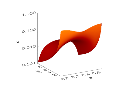
Figure 3: The coefficients ${\kappa_{{}_{B,EE}}}$ for linear-experiment gain errors, plotted as a function of polarizer angle $\alpha$ and antenna separation $u\sigma$. The left plot is for the parameter $\mathop{\rm Re}(\gamma_{2})$, and the right is for $\mathop{\rm Im}(\gamma_{2})$. The coefficient for $\gamma_{1}$ has no $\alpha$-dependence and so is not plotted here (but see Fig. 4).

Suppose that there is an error (e.g., a gain error) in the data, but we don’t know it. Since we think we are dealing with an error-free experiment, we use the optimal prescription (34) to estimate the power spectra from a single set of visibilities. The presence of the systematic error will alter the covariances (36) and hence the statistical properties of the estimators. Let $\delta\hat{C}^{K}$ with $K=\{E,B\}$ be the difference between the estimate we actually get and what we would have gotten in the absence of systematic errors:

$$\delta\hat{C}^{K}=\hat{C}^{K}_{\rm actual}-\hat{C}^{K}_{\rm no\ errors}.$$ (41)

It is natural to use the r.m.s. values of these differences,

$$\delta\hat{C}^{K}_{\rm rms}=\langle(\delta\hat{C}^{K})^{2}\rangle^{1/2},$$ (42)

to quantify the effect of each systematic error on the power spectrum estimates. We focus for the moment on the case of “instrument errors” as described in Section III.1, deferring the generalization to beam errors until section VI.

The effect of each instrument error is to mix together the Stokes visibilities $V_{I},V_{Q},V_{U}$ in a linear fashion (neglecting circular polarization for the present). If ${\bf v}$ denotes the vector of Stokes visibilities that would be obtained without systematic errors, the vector actually observed is

$${\bf v}^{\prime}={\bf v}+\delta{\bf v}={\bf v}+{\bf E}\cdot{\bf v}$$ (43)

for some $3\times 3$ matrix ${\bf E}$.

The error in the power spectrum estimates is

$$\delta\hat{C}^{K}=({\bf v}+\delta{\bf v})^{\dagger}\cdot{\bf N}_{K}\cdot({\bf v}+\delta{\bf v})-{\bf v}^{\dagger}\cdot{\bf N}_{K}\cdot{\bf v}.$$ (44)

Assuming that the errors are small, we can neglect the term that is quadratic in $\delta{\bf v}$:

$$\delta\hat{C}^{K}={\bf v}^{\dagger}\cdot({\bf E}^{\dagger}\cdot{\bf N}_{K}+{\bf N}_{K}\cdot{\bf E})\cdot{\bf v}\equiv{\bf v}^{\dagger}\cdot{\bf A}_{K}\cdot{\bf v}.$$ (45)

Assuming Gaussian fluctuations, there is a relatively simple expression for the variance of this quantity, as shown in the Appendix:

$$(\delta\hat{C}^{K}_{\rm rms})^{2}={\rm Tr}[({\bf A}_{K}\cdot{\bf M}_{v})^{2}]+[{\rm Tr}({\bf A}_{K}\cdot{\bf M}_{v})]^{2}.$$ (46)

As noted in the previous subsection, when these formulae are applied to visibilities in a coordinate system that is not aligned with the baseline vector, we must correct them by conjugating with the matrix ${\bf R}$. All that is necessary is to replace the error matrix ${\bf E}$ with

$${\bf E}\to{\bf R}\cdot{\bf E}\cdot{\bf R}^{-1}.$$ (47)

For any particular source of error, we now have a recipe for calculating the effect on the power spectrum: we write down an explicit form for the matrix ${\bf E}$ and apply equation (46). The result will be a sum of terms that are quadratic in the band powers $C^{T},C^{X},C^{E},C^{B}$. All of these quantities represent band powers at the same multipole $l=2\pi u$; we continue to omit the multipole subscript $2\pi u$ throughout this section for simplicity. In particular, the error in our estimate of the $B$-mode band power generically looks like

$$(\delta\hat{C}^{B}_{\rm rms})^{2} =\sum_{I,J}\eta^{B}_{IJ}C^{I}C^{J}$$ (48a)

$$=\eta^{B}_{TT}(C^{T})^{2}+\eta^{B}_{TX}C^{T}C^{X}+\eta^{B}_{TE}C^{T}C^{E}+\ldots$$

$$\qquad\qquad+\eta^{B}_{EE}(C^{E})^{2}+\ldots.$$ (48b)

Each of the coefficients $\eta$ depends on the various parameters that characterize the instrument errors, such as the gain fluctuations $g_{i}^{(j)}$ and couplings $\epsilon_{i}^{(j)}$. Of course, a similar expression would apply to $\hat{C}^{E}$.

We now imagine “turning on” one error at a time. Consider a systematic error characterized by a single parameter $p$. The coefficients $\eta$ in the above expression will contain terms proportional to $p^{2}$ at leading order, because equation (46) is quadratic in the error matrix ${\bf E}$:

$$\eta^{K}_{IJ}={\kappa^{2}_{{}_{K,IJ,p}}}p_{\rm rms}^{2}.$$ (49)

Here $K=\{E,B\}$ is the power spectrum we are trying to estimate; and $I,J=\{T,X,E,B\}$ are the power spectra being coupled to our estimate.

Equations (48b) and (49) together yield the key result of this section:

$$(\delta\hat{C}_{\rm rms}^{K})^{2}=p_{\rm rms}^{2}\sum_{I,J}{\kappa^{2}_{{}_{K,IJ,p}}}C^{I}C^{J}.$$ (27)

We will drop the subscript rms on $p$ below.

For any given type of error, of course, some of the coefficients $\eta$ will vanish. For instance, as we saw earlier, gain errors do not couple $I$ to $Q,U$, so there will be no contributions coupling $C^{T}$ or $C^{X}$ to the polarization band power estimates. Since there is a clear hierarchy $C^{T}>C^{X}>C^{E}>C^{B}$ (see Fig. 1), it often makes sense for each error to consider only the term in (27) that contains the biggest power spectra.

Figure 4: Coefficients $\kappa$ averaged over $\alpha$ for linear-experiment gain fluctuations. The left plot shows ${\kappa_{{}_{B,EE}}}$ for the three independent gain fluctuation parameters $\mathop{\rm Re}(\gamma_{1}),\mathop{\rm Re}(\gamma_{2}),\mathop{\rm Im}(\gamma_{2})$ as defined in equation (53). The right plot shows the coefficients ${\kappa_{{}_{B,EB}}}$. In each case, the dashed curves show the leading term in a Taylor series in $\overline{s^{2}}$, which is generally a good approximation. The vertical dotted line at $u\sigma=0.52$ corresponds to antennas that are touching.

For any one source of error, the fractional error on the band power will be

$$\frac{\delta\hat{C}^{K}_{\rm rms}}{C^{K}}=p{\kappa_{{}_{K,IJ,p}}}\frac{\sqrt{C^{I}C^{J}}}{C^{K}},$$ (50)

assuming that one term in the sum (27) dominates the error. If we demand that this fractional error be below some specified tolerance, then we can determine the required specification for the input parameter $p$. The coefficients $\kappa$ are thus the key to assessing the severity of any particular source of systematic error. The next sections present calculations of these coefficients.

V Results: Instrument errors

This section presents the results of applying the above formalism to the various instrument errors described in section III.1. Beam errors will be treated in the following section. There are several cases to consider. A table summarizing the key results, along with a discussion of their implications, may be found in Section VII.

Gain errors: Linear experiment: Consider an experiment that measures linear polarization states, and assume that there are gain errors $g_{i}^{(j)}$, ignoring couplings ($\epsilon_{i}^{(j)}$) for the present. As equation (19) shows, the resulting error in each visibility is simply proportional to the visibility itself: $\delta V_{Q}=\gamma_{Q}V_{Q}$ and $\delta V_{U}=\gamma_{U}V_{U}$. Here

$$\gamma_{Q,U}=\tfrac{1}{2}(g_{1}^{(j)}+g_{2}^{(j)}+g_{1}^{(k)*}+g_{2}^{(k)*}),$$ (51)

with the parameters $g_{i}^{(j)}$ evaluated at the time the corresponding visibility is measured. If $V_{Q},V_{U}$ are measured with the same antennas (by rotating the polarizers in each antenna $45^{\circ}$), and if they are measured at nearly the same time so that the gains have not drifted, then $\gamma_{Q}=\gamma_{U}$. It is far more likely, however, that the two visibilities have independent gain fluctuations, in which case $\gamma_{Q}$ and $\gamma_{U}$ should be treated as independent, unknown error parameters.

In the notation of the previous subsection, we can characterize these errors with a matrix

$${\bf E}=\begin{pmatrix}0&0&0\\ 0&\gamma_{1}+\frac{1}{2}\gamma_{2}&0\\ 0&0&\gamma_{1}-\frac{1}{2}\gamma_{2}\end{pmatrix},$$ (52)

where

$$\gamma_{1}=\tfrac{1}{2}(\gamma_{Q}+\gamma_{U}),\qquad\gamma_{2}=\tfrac{1}{2}(\gamma_{Q}-\gamma_{U}).$$ (53)

In general, we will concern ourselves only with errors that couple larger power spectra to smaller ones. In an experiment to measure $E$ modes, gain fluctuations do not lead to any such terms. We therefore focus on a $B$ mode experiment. If we use this matrix to calculate the errors on the $B$ power spectrum, the leading term is the $EE$ term:

$$(\delta\hat{C}_{\rm rms}^{B})^{2}=\eta^{B}_{EE}(C^{E})^{2}+\ldots.$$ (54)

The coefficient is

$$\eta^{B}_{EE} =\frac{\overline{s^{2}}\,\overline{c^{2}}}{2(\overline{c^{2}}-\overline{s^{2}})^{2}}\bigl{[}|\gamma_{2}|^{2}\sin^{2}(4\alpha)+$$

$$4\overline{s^{2}}\,\overline{c^{2}}(4\mathop{\rm Re}(\gamma_{1})^{2}+(3-4\sin^{2}(4\alpha))\mathop{\rm Re}(\gamma_{2})^{2})\bigr{]}.$$ (55)

The baseline vector ${\bf u}$ makes an angle $\alpha$ with the $x$ axis.

The effect is characterized by three parameters $\gamma_{1r}=\mathop{\rm Re}(\gamma_{1})$, $\gamma_{2r}=\mathop{\rm Re}(\gamma_{2})$, $\gamma_{2i}=\mathop{\rm Im}(\gamma_{2})$. The coefficients associated with these parameters are

$${\kappa^{2}_{{}_{B,EE,\gamma_{1r}}}} =\frac{8(\overline{s^{2}}\,\overline{c^{2}})^{2}}{(\overline{c^{2}}-\overline{s^{2}})^{2}},$$ (56a)

$${\kappa^{2}_{{}_{B,EE,\gamma_{2r}}}} =\frac{\overline{s^{2}}\,\overline{c^{2}}}{2(\overline{c^{2}}-\overline{s^{2}})^{2}}[\sin^{2}(4\alpha)+$$

$$\qquad 4(3\cos^{2}(4\alpha)-\sin^{2}(4\alpha))\overline{s^{2}}\,\overline{c^{2}}],$$ (56b)

$${\kappa^{2}_{{}_{B,EE,\gamma_{2i}}}} =\frac{\overline{s^{2}}\,\overline{c^{2}}\sin^{2}(4\alpha)}{2(\overline{c^{2}}-\overline{s^{2}})^{2}}.$$ (56c)

We can simplify these expressions and those to follow in two ways. First, since a typical experiment will involve visibilities measured with many different baseline orientations, we will generally average over the angle $\alpha$. Second, since $\overline{s^{2}}$ is generally a small quantity, we can often keep only the leading term in a Taylor expansion in $\overline{s^{2}}$. In these approximations, the coefficients simplify to

$${\kappa_{{}_{B,EE,\gamma_{1r}}}} =\sqrt{8}\ \overline{s^{2}},$$ (57a)

$${\kappa_{{}_{B,EE,\gamma_{2r}}}} ={\kappa_{{}_{\gamma_{2i}}}}=\tfrac{1}{2}\sqrt{\overline{s^{2}}}.$$ (57b)

Figure 3 shows the coefficients associated with $\gamma_{2}$ as functions of both $\alpha$ and antenna separation $u\sigma$ (which determines $\overline{s^{2}}$). Figure 4 shows the result of averaging over $\alpha$, as well as the $\gamma_{1r}$ coefficient, which is independent of $\alpha$. As the figure indicates, the leading-order approximation in $\overline{s^{2}}$ is quite good.

We should consider whether it is always adequate to keep only the leading term $\eta^{B}_{EE}$. The full expression for the power spectrum error contains a term $\eta^{B}_{EB}$ as well. The fractional error caused by this term scales as only $\sqrt{C^{E}/C^{B}}$ rather than $C^{E}/C^{B}$ (eq. 50). However, the coefficient ${\kappa_{{}_{B,EE}}}$ can be small (see Fig. 4), especially for widely separated antennas. As the right panel of Fig. 4 shows, the coefficient $\kappa_{B,EB}$ can be much larger than $\kappa_{B,EE}$. Determination of which term dominates must unfortunately be made on a case-by-case basis.

Figure 5: Coefficients for gain errors in a circular-polarization experiment with parameters defined in (59). As in Fig. 4, the left plot shows the coefficients ${\kappa_{{}_{B,EE}}}$, and the right shows ${\kappa_{{}_{B,EB}}}$. Dashed lines indicate the leading-order approximation in $\overline{s^{2}}$. These coefficients are independent of $\alpha$, so no averaging was necessary. The vertical dotted line corresponds to antennas that are touching.

The size of the coefficient $\kappa$ is largely determined by its dependence on the small parameter $\overline{s^{2}}$. As a general rule, we need to weigh the importance of a subdominant contribution to the error (i.e., one that ranks lower in the $T,X,E,B$ hierarchy) if that error has a weaker dependence on $\overline{s^{2}}$. In the case of the parameter $\gamma_{1}$, for example, the EE term has ${\kappa_{{}_{B,EE}}}\propto\overline{s^{2}}$ but ${\kappa_{{}_{B,EB}}}\propto\sqrt{\overline{s^{2}}}$. For $\gamma_{2}$, the EB coefficient has an $\overline{s^{2}}$-independent term. Thus for small $\overline{s^{2}}$ (large separation), the EB terms may become more important than the EE terms. See Section VII and especially Table 1 for further discussion of this point.

Gain errors: Circular experiment: In this case, we assume an experiment that measures $V_{Q}$ and $V_{U}$ simultaneously by interfering right and left circular polarizations. Again, we focus on an experiment to measure $B$ modes, as gain errors do not pose a serious problem in an $E$ mode experiment. From equations (21), we see that gain errors $g_{i}^{(j)}$ produce an error matrix of the form

$${\bf E}=\begin{pmatrix}0&0&0\\ 0&\gamma_{1}&i\gamma_{2}\\ 0&-i\gamma_{2}&\gamma_{1}\end{pmatrix},$$ (58)

where

$$\gamma_{1} =\tfrac{1}{2}(g_{1}^{(j)}+g_{2}^{(j)}+g_{1}^{(k)*}+g_{2}^{(k)*}),$$ (59a)

$$\gamma_{2} =\tfrac{1}{2}(g_{1}^{(j)}-g_{2}^{(j)}-g_{1}^{(k)*}+g_{2}^{(k)*}).$$ (59b)

As in the previous case, the dominant error contribution to a measurement of $B$ power is the $EE$ term:

$$\eta_{EE}^{B}=\frac{2\overline{s^{2}}\,\overline{c^{2}}(|\gamma_{2}|^{2}+4\overline{s^{2}}\,\overline{c^{2}}(\mathop{\rm Re}(\gamma_{1})^{2}-\mathop{\rm Re}(\gamma_{2})^{2}))}{(\overline{c^{2}}-\overline{s^{2}})^{2}}.$$ (60)

The coefficients are

$${\kappa^{2}_{{}_{B,EE,\gamma_{1r}}}} =\frac{8(\overline{s^{2}}\,\overline{c^{2}})^{2}}{(\overline{c^{2}}-\overline{s^{2}})^{2}}\approx 8(\overline{s^{2}})^{2},$$ (61a)

$${\kappa^{2}_{{}_{B,EE,\gamma_{2r}}}} =\frac{2\overline{s^{2}}\,\overline{c^{2}}(1-4\overline{s^{2}}\,\overline{c^{2}})}{(\overline{c^{2}}-\overline{s^{2}})^{2}}\approx 2\overline{s^{2}},$$ (61b)

$${\kappa^{2}_{{}_{B,EE,\gamma_{2i}}}} =\frac{2\overline{s^{2}}\,\overline{c^{2}}}{(\overline{c^{2}}-\overline{s^{2}})^{2}}\approx 2\overline{s^{2}},$$ (61c)

where the approximate equalities are the leading terms in an expansion in $\overline{s^{2}}$. See Figure 5.

As in the case of a linear polarization experiment, the $EB$ error term can become dominant for widely-separated antennas. In particular, for the parameter $\gamma_{2}$ the EB coefficient has a term independent of $\overline{s^{2}}$: ${\kappa_{{}_{B,EB,\gamma_{2r,i}}}}=\sqrt{2}$ to leading order in $\overline{s^{2}}$.

Couplings: Next we turn to errors parameterized by the “coupling” terms $\epsilon_{i}^{(j)}$ in the instrument Jones matrix. These errors include electronic cross-talk as well as errors in the alignments of the polarizers in a linear experiment. In both linear and circular experiments, these errors couple $I$ into $Q,U$, so the dominant terms will be those involving the temperature power spectrum. In this section, unlike the previous ones, we should consider $E$ as well as $B$ mode experiments.

The error matrix characterizing $I\to Q,U$ leakage in this situation is

$${\bf E}=\begin{pmatrix}0&0&0\\ \varepsilon_{1}&0&0\\ \varepsilon_{2}&0&0\end{pmatrix}.$$ (62)

Here $\varepsilon_{1},\varepsilon_{2}$ are the coefficients of $\accentset{\circ}{V}_{I}$ in equations (19) and (21): For a linear experiment,

$$\varepsilon_{1,2}=\tfrac{1}{2}(\epsilon_{1}^{(j)}+\epsilon_{2}^{(j)}+\epsilon_{1}^{(k)*}+\epsilon_{2}^{(k)*}),$$ (63)

with the parameters $\epsilon_{i}^{(j)}$ evaluated when the corresponding visibility is measured. For a circular experiment,

$$\varepsilon_{1} =\tfrac{1}{2}(\epsilon_{1}^{(j)}+\epsilon_{2}^{(j)}+\epsilon_{1}^{(k)*}+\epsilon_{2}^{(k)*}),$$ (64a)

$$\varepsilon_{2} =\tfrac{1}{2}(-\epsilon_{1}^{(j)}+\epsilon_{2}^{(j)}+\epsilon_{1}^{(k)*}-\epsilon_{2}^{(k)*}).$$ (64b)

In the linear case, there are also terms that couple $Q$ and $U$. We omit these, as the errors they produce are always small in comparison to the terms involving $I$.

Consider first a $B$ mode experiment. The $TT$ and $TX$ terms in (48b) vanish, so the dominant contribution is the $TE$ term. After averaging over $\alpha$, this term is

$$\eta_{TE}^{B}=\frac{\overline{s^{2}}\,\overline{c^{2}}(|\varepsilon_{1}|^{2}+|\varepsilon_{2}|^{2})}{(\overline{c^{2}}-\overline{s^{2}})^{2}},$$ (65)

so the coefficients for the parameters $\mathop{\rm Re}(\varepsilon_{1}),\mathop{\rm Im}(\varepsilon_{1}),\mathop{\rm Re}(\varepsilon_{2}),\mathop{\rm Re}(\varepsilon_{2})$ are

$${\kappa^{2}_{{}_{B,TE,\varepsilon}}}=\frac{\overline{s^{2}}\,\overline{c^{2}}}{(\overline{c^{2}}-\overline{s^{2}})^{2}}\approx\overline{s^{2}},$$ (66)

as shown in Figure 6. The $TB$ term has an $\overline{s^{2}}$-independent piece:

$${\kappa^{2}_{{}_{B,TB,\varepsilon}}}=\frac{1+3\overline{s^{2}}\,\overline{c^{2}}}{(\overline{c^{2}}-\overline{s^{2}})^{2}}\approx 1,$$ (67)

which can be important for large antenna separation. See Table 1.

The coefficients for an $E$ mode experiment are the same as for a $B$ mode experiment with $E$ and $B$ switched. The dominant contribution is therefore ${\kappa_{{}_{E,TE}}}\approx 1$.

Figure 6: Coefficients for coupling errors parameterized as in equations (63) and (64). Dashed and dotted curves are as in the previous figures.

VI Beam errors

In section IV.3, we derived a method of forecasting the effects of instrument errors on power spectrum estimates. We now generalize this method to the case of beam errors.

In the case of instrument errors, we were able to write the errors in the visibilities as $\delta{\bf v}={\bf E}\cdot{\bf v}$, where the error matrix ${\bf E}$ depended only on the unknown error parameters. Beam errors cannot be treated in this way. Both $\delta{\bf v}$ and ${\bf v}$ are integrals over the Stokes parameters, but with different weightings in Fourier space. As a result, one is not a simple linear transformation of the other. Fortunately, for a number of important sources of error, the differences in Fourier-space weighting are modest: the errors sample roughly if not exactly the same regions of the Fourier plane. We can therefore still express our final results in the form (27), after we have made some adaptation to the formalism of section IV.3.

Combine ${\bf v}$ and $\delta{\bf v}$ together into a 6-dimensional vector ${\bf w}=({\bf v},\delta{\bf v})=(V_{I},V_{Q},V_{U},\delta V_{I},\delta V_{Q},\delta V_{U})$. To leading order in $\delta{\bf v}$, the error in the power spectrum estimate is

$$\delta\hat{C}^{K}={\bf w}^{\dagger}\cdot{\cal N}_{K}\cdot{\bf w},$$ (68)

where $K=\{E,B\}$ and the matrix ${\cal N}$ can be written in block form as

$${\cal N}_{K}=\begin{pmatrix}0&{\bf N}_{K}\\ {\bf N}_{K}&0\end{pmatrix},$$ (69)

with ${\bf N}_{K}$ the same as for instrument errors. It is straightforward to check that this reduces to (44).

Using the identity proved in the Appendix again, we can write

$$(\delta\hat{C}^{K}_{\rm rms})^{2}=\mathop{\rm Tr}\left[({\cal N}_{K}\cdot{\bf M}_{w})^{2}\right]+\left[\mathop{\rm Tr}({\cal N}_{K}\cdot{\bf M}_{w})\right]^{2},$$ (70)

where ${\bf M}_{w}=\langle{\bf w}\cdot{\bf w}^{\dagger}\rangle$ is the covariance matrix of the vector ${\bf w}$. We now need a recipe for calculating the elements of this covariance matrix, which will contain terms proportional to the various power spectra.

In sections II.2 and III.2, we expressed each component of ${\bf v}$ and $\delta{\bf v}$ as an integral over the Stokes parameters. To be explicit, let ${\bf s}({\bf k})=(\tilde{I}({\bf k}),\tilde{Q}({\bf k}),\tilde{U}({\bf k}))$ be a vector giving the Fourier-space Stokes parameters. Each component of ${\bf w}$ can be expressed in the form

$$w_{i}=\int d^{2}k\,{\bf W}_{i}({\bf k})\cdot{\bf s}({\bf k})$$ (71)

for some vector-valued window function ${\bf W}_{i}$. A covariance matrix $\langle w_{i}w_{j}^{*}\rangle$ then becomes an integral over ${\bf k}$ of the two window functions times the covariances of the Stokes parameters $\langle{\bf s}\cdot{\bf s}^{\dagger}\rangle$. The latter are proportional to the input power spectra. So once we have written down the window functions for the visibilities and their associated systematic errors, we can calculate an expression giving contributions to the error $\delta\hat{C}^{K}_{\rm rms}$ in terms of the input power spectra, just as in the case of instrument errors. For some parameterizations of beam errors, the resulting integrals can be performed analytically to yield closed-form expressions like those in the previous section for the coefficients $\kappa$. However, the resulting expressions are complicated and unenlightening, so we present the results of numerical integration instead.

As in the previous section, we now examine detailed case-by-case results. Section VII provides a summary of the implications.

As noted earlier, the set of possible forms for beam errors is dauntingly large. Our treatment will necessarily be restricted to a small set of physically motivated possibilities rather than exploring the entire space. As in the previous section, we will imagine turning on one error at a time.

Differential pointing errors (“squint”): Suppose that some antennas have slight pointing offsets relative to others. This situation can be treated as a beam mismatch error as in equation (22).

Let $A_{0}(\hat{\bf r})$ be the antenna pattern in the absence of the pointing errors, which we will take to be a Gaussian. Then in the notation of equation (22), the antenna pattern for the $j$th antenna is

$$A^{(j)}(\hat{\bf r})=A(\hat{\bf r}+\delta\hat{\bf r}_{j}),$$ (72)

where $\delta\hat{\bf r}_{j}$ is the pointing error of the $j$th antenna. Using equations (23), we find that each visibility looks like

$$V_{Z}=\int d^{2}\hat{\bf r}e^{-2\pi i{\bf u}_{jk}\cdot\hat{\bf r}}Z(\hat{\bf r})A^{(j)}(\hat{\bf r})A^{(k)*}(\hat{\bf r}),$$ (73)

where $Z=\{Q,U\}$. The product of two Gaussians is a Gaussian centered at the midpoint of the two: $A^{(j)}(\hat{\bf r})A^{(k)}(\hat{\bf r})\propto\exp[-(\hat{\bf r}-\frac{1}{2}(\delta\hat{\bf r}_{j}+\delta\hat{\bf r}_{k})^{2})/(2\sigma^{2})]$. That is, each visibility is calculated using an effective beam pattern that is shifted by the average of the shifts of the two antennas. For any given antenna pair $(jk)$, we define an error parameter

$$\bm{\delta}_{jk}=\frac{\delta\hat{\bf r}_{j}+\delta\hat{\bf r}_{k}}{2\sigma},$$ (74)

the average of the two antennas’ pointing errors in units of the beam width.

Figure 7: Error coefficients for beam pointing errors. The quantity $\bm{\delta}_{+}$ is a common pointing error (the same for both $V_{Q},V_{U}$), while $\bm{\delta}_{-}$ is a relative pointing error. Both $\bm{\delta}_{\pm}$ are measured in units of the beam width. Results are averaged over directions of $\bm{\delta}_{\pm}$. Furthermore, in the case of $\bm{\delta}_{-}$, an average has been taken over the angle $\alpha$ between ${\bf u}$ and the $x$ axis. Dashed and dotted curves are as in the previous figures.

Shifting a function by an amount $\bm{\Delta}$ is equivalent to multiplying its Fourier transform by $e^{i{\bf k}\cdot\bm{\Delta}}$, so by (14) the visibility is

$$V_{Z}=\int d^{2}k\,\tilde{Z}({\bf k})\widetilde{A_{0}^{2}}({\bf k}-2\pi{\bf u})^{*}e^{-i({\bf k}-2\pi{\bf u})\cdot\bm{\delta}_{jk}\sigma}.$$ (75)

To leading order in $\bm{\delta}_{jk}$, the error is

$$\delta V_{Z}=-i\int d^{2}k\,\tilde{Z}({\bf k})\widetilde{A_{0}^{2}}({\bf k}-2\pi{\bf u})^{*}({\bf k}-2\pi{\bf u})\cdot\bm{\delta}_{jk}\sigma.$$ (76)

As before, we imagine a single measurement pair $(V_{Q},V_{U})$ corresponding to the same baseline ${\bf u}$. Let $\bm{\delta}_{Q}$ be the value of $\bm{\delta}_{jk}$ corresponding to the visibility $V_{Q}$ and $\bm{\delta}_{U}$ be the value corresponding to $V_{U}$. In a circular experiment, the two visibilities are measured with the same antenna pair, so $\bm{\delta}_{Q}=\bm{\delta}_{U}$, while in a linear experiment they should be regarded as independent error parameters. It is convenient to express our final results in terms of the sum and difference,

$$\bm{\delta}_{\pm}=\tfrac{1}{2}(\bm{\delta}_{Q}\pm\bm{\delta}_{U}).$$ (77)

In a circular experiment, $\bm{\delta}_{-}=0$.

We can now calculate the various correlations $\langle\delta V_{Q}V_{Q}\rangle$, etc., by integrating over ${\bf k}$. The result will contain terms proportional to the band powers $C_{2\pi u}^{E},C_{2\pi u}^{B}$, and quadratic in the parameters $\bm{\delta}_{+},\bm{\delta}_{-}$. We can therefore define parameters $\kappa$ characterizing these errors exactly as in the case of instrument errors [equation (27)].

As in the previous cases, the severity of the errors depends on $\overline{s^{2}}$, which characterizes the degree of $EB$ mixing within each visibility pair. Furthermore, the components of $\bm{\delta}_{\pm}$ parallel and perpendicular to the baseline, $\delta_{\pm\parallel}$ and $\delta_{\pm\perp}$, contribute differently. Finally, in the case of $\bm{\delta}_{-}$, the results depend on the angle $\alpha$ between the baseline and the coordinate axis. For simplicity, we have averaged over both components $\delta_{\parallel}$ and $\delta_{\perp}$ for each of $\bm{\delta}_{\pm}$, and we have also averaged over $\alpha$. Figure 7 illustrates the resulting coefficients. As before, the coefficients are well approximated by the leading-order terms in an expansion in $\overline{s^{2}}$, which are given in Table 1. Not surprisingly, $\bm{\delta}_{-}$ is a greater source of error than $\bm{\delta}_{+}$. As comparison with Figures 4 and 5 indicates, the effects of differential pointing errors ($\bm{\delta}_{-}$) are generally similar to those of gain errors.

Beam shape errors: Equation (22) can also be used to model errors in the beam shape. To illustrate this, we consider Gaussian beams with errors in the beam width.

Assume that in an ideal, error-free experiment all antennas have azimuthally symmetric Gaussian beam patterns with beam width $\sigma$. Suppose that in actuality each antenna has an elliptical beam pattern with different beam widths $\sigma_{1}^{(j)},\sigma_{2}^{(j)}$ along its two principal axes. As equation (23) indicates, the effective beam pattern for each visibility $V^{(jk)}$ is just the product of the two antenna patterns. The product of Gaussians is a Gaussian, so the effective visibility beam pattern will be of the form

$$A^{(j)}(\hat{\bf r})A^{(k)}(\hat{\bf r})\propto\exp[{-\hat{\bf r}\cdot(\bm{1}+\bm{\Delta}_{jk})\cdot\hat{\bf r}/(2\sigma^{2})}].$$ (78)

Here the symmetric $2\times 2$ matrix $\bm{\Delta}_{jk}$ characterizes the deviation of the beam from the ideal symmetric Gaussian of width $\sigma$. To be specific, the eigenvectors of $\bm{\Delta}_{jk}$ give the two principal axes of the elliptical beam, and the beam widths are $\sigma/\sqrt{1+\lambda_{i}}$ where $\lambda_{1},\lambda_{2}$ are the eigenvalues. We will assume that the errors are small and work to leading order in $\lambda_{i}$. The fractional errors in the beam width in the two principal directions are then $\delta\sigma_{i}/\sigma=-\lambda_{i}/2$, where $i=1,2$ label the two principal axes of the beam.

As usual we consider a visibility pair $(V_{Q},V_{U})$ measured with a common baseline ${\bf u}$. In the case of a linear experiment, the two visibilities may be measured with different antenna pairs, so we should consider two sets of beam shape parameters characterized by matrices $\bm{\Delta}_{Q},\bm{\Delta}_{U}$. In a circular experiment where both visibilities are measured simultaneously with a single antenna pair, $\bm{\Delta}_{Q}=\bm{\Delta}_{U}$. As we have seen before, we can treat both cases simultaneously by defining

$$\bm{\Delta}_{\pm}=\tfrac{1}{2}(\bm{\Delta}_{Q}\pm\bm{\Delta}_{U}).$$ (79)

The matrix $\bm{\Delta}_{+}$ characterizes the average beam shape when the two visibilities are measured, and $\bm{\Delta}_{-}$ characterizes errors in beam shape that differ between $V_{Q},V_{U}$. In both cases, the two eigenvalues of the matrices give fractional errors in beam width in the two principal directions:

$$\zeta_{\pm,i}\equiv\frac{\delta\sigma_{\pm,i}}{\sigma}=-\frac{\lambda_{\pm,i}}{2}.$$ (80)

Here $i=1,2$ labels the two principal axes for each of $\bm{\Delta}_{\pm}$.

Figure 8: Error coefficients for beam shape errors, parameterized by the coefficients $\zeta_{+,i}$ (“common”) and $\zeta_{-,i}$ (“diff.”) in equation (80). Dashed and dotted curves are as in previous figures.

We will refer to errors parameterized by $\zeta_{+,i}$ as common beam shape errors and to those parameterized by $\zeta_{-,i}$ as differential errors. For a circular experiment we expect differential errors to vanish, while for a linear experiment both should be of comparable magnitude. We will consider separately the effects of common and differential errors.

In each of the two cases, there are three parameters: $\zeta_{1},\zeta_{2}$, and an angle $\beta$ giving the orientation of the principal axes relative to the coordinate axes used to define $Q,U$. For common errors, the results are independent of $\beta$, but for differential errors they depend on $\beta$ (unless $\zeta_{-,1}=\zeta_{-,2}$, in which case there is rotational symmetry). We assume that the principal axes are randomly oriented, so we average over $\beta$ in the results below.

For both common and differential errors, there are two qualitatively different possibilities one might wish to consider. If $\zeta_{1}=\zeta_{2}$, then the beam is circular, and we have made an error only in its width. On the other hand, the case $\zeta_{1}=-\zeta_{2}$ corresponds to a pure beam shape error, with the beam stretched along one axis and squeezed equally along the other. Of course, the most general case would be a combination of the two. The final results (after averaging over $\beta$ where appropriate) turn out to be the same in both cases: the error depends only on the combination $\zeta_{1}^{2}+\zeta_{2}^{2}$ regardless of the relative signs.

Figure 8 shows the coefficients $\kappa$ associated with beam shape errors. The results are quite similar to those for pointing errors. In particular, the differential errors that arise in a linear experiment are more severe than the common errors, which arise in both linear and circular experiments.

Figure 9: Coefficients for cross-polar beam response, parameterized by $\mu_{Q},\mu_{U}$ [eq. (82)]. Dashed and dotted curves are as in previous figures.

Experiment	Measurement	Error	Dominant	Fiducial	Secondary	Fiducial
type		source	contribution	$\delta\hat{C}/C$	contribution	$\delta\hat{C}/C$
Linear	$B$	Gain error	${\kappa_{{}_{B,EE,\gamma_{2}}}}=\frac{1}{2}\sqrt{\overline{s^{2}}}$	$21\gamma_{2}$	${\kappa_{{}_{B,EB,\gamma_{2}}}}=\frac{1}{2}$	$8.7\gamma_{2}$
Circular	$B$	Gain error	${\kappa_{{}_{B,EE,\gamma_{2}}}}=\sqrt{2\overline{s^{2}}}$	$60\gamma_{2}$	${\kappa_{{}_{B,EB,\gamma_{2}}}}=\sqrt{2}$	$24\gamma_{2}$
Linear/Circular	$B$	Coupling	${\kappa_{{}_{B,TE,\varepsilon}}}=\sqrt{\overline{s^{2}}}$	$730\varepsilon$	${\kappa_{{}_{B,TB,\varepsilon}}}=1$	$300\varepsilon$
Linear/Circular	$E$	Coupling	${\kappa_{{}_{E,TE,\varepsilon}}}=1$	$17\varepsilon$	—	—
Linear	$B$	Pointing	${\kappa_{{}_{B,EE,\delta_{-}}}}=\sqrt{\overline{s^{2}}/2}$	$30\delta_{-}$	${\kappa_{{}_{B,EB,\delta_{-}}}}=1$	$17\delta_{-}$
Circular	$B$	Pointing	${\kappa_{{}_{B,EE,\delta_{+}}}}=\sqrt{8}\overline{s^{2}}$	$17\delta_{+}$	${\kappa_{{}_{B,EB,\delta_{+}}}}=\sqrt{6\overline{s^{2}}}$	$6\delta_{+}$
Linear	$B$	Beam shape	${\kappa_{{}_{B,EE,\zeta_{-}}}}=\sqrt{\overline{s^{2}}}$	$42\zeta_{-}$	${\kappa_{{}_{B,EB,\zeta_{-}}}}=1$	$17\zeta_{-}$
Circular	$B$	Beam shape	${\kappa_{{}_{B,EE,\zeta_{+}}}}=3.5\overline{s^{2}}$	$21\zeta_{+}$	${\kappa_{{}_{B,EB,\zeta_{+}}}}=\sqrt{8\overline{s^{2}}}$	$7\zeta_{+}$
Linear/Circular	$B$	Cross-polarization	${\kappa_{{}_{B,TE,\mu}}}=\sqrt{\overline{s^{2}}}$	$730\mu$	${\kappa_{{}_{B,TB,\mu}}}=1$	$300\mu$
Linear/Circular	$E$	Cross-polarization	${\kappa_{{}_{E,TE,\mu}}}=1$	$17\mu$	—	—

Table 1: Effects of instrument errors (above line) and beam errors (below line). See Section VII for details.

Cross-polarization: The final case we consider is azimuthally-symmetric cross-polarization, with antenna patterns of the form (25). We consider an ideal experiment to be one with cross-polar terms $A_{1}^{(i)}=0$ for all antennas. The error term can in principle be an arbitrary function of $r$. We generally expect cross-polar response to be small near the beam center, so we adopt the following simple form for the cross-polar response:

$$A_{1}^{(i)}(r)=\mu_{i}\frac{r^{2}}{\sigma^{2}}A_{0}(r),$$ (81)

where $A_{0}$ is assumed to have the usual Gaussian form and $\mu_{i}$ is the parameter characterizing the size of the error.

As an aside, note that this particular form arises in one simple model of an antenna. Suppose the antenna lies in the $xy$ plane and responds equally to both $x$ and $y$ components of the incoming electric field, with no sensitivity to the $z$ component. In the flat-sky limit such an antenna has no cross-polar response, but sky curvature introduces cross-polarization of this form (because $E_{\theta}$ is reduced a factor of $\cos\theta\approx 1-\frac{1}{2}\theta^{2}$ upon projection onto the $xy$ plane, while $E_{\phi}$ is unchanged). This cross-polarization is characterized by $\mu=\frac{1}{2}\sigma^{2}$ with $\sigma$ in radians. (Incidentally, when sky curvature is taken into account one must be careful to distinguish among inequivalent definitions of “cross-polarization.” The most natural one in this context, because it respects azimuthal symmetry, is “definition 3” in ref. Ludwig (1973).)

The relevant quantity for characterizing the error in each of the visibilities $V_{Q},V_{U}$ is

$$\mu_{Q,U}=\tfrac{1}{2}(\mu_{j}+\mu_{k}),$$ (82)

the average of the two $\mu$ parameters when each of $V_{Q},V_{U}$ is measured. As usual, for a circular experiment $\mu_{Q}=\mu_{U}$ while in a linear experiment the two are independent. In this case, however, it makes no difference which case we consider, as the error contributions due to $\mu_{Q},\mu_{U}$ simply add independently (in quadrature).

Figure 9 shows the leading error coefficients for this case. Since these errors couple $I$ into $Q,U$, the dominant terms are those involving the temperature power spectrum, and errors can be quite significant for both $E$ and $B$ measurements.

VII Discussion

This paper has presented a method of quantifying the effects of a variety of systematic errors on estimates of the CMB polarization power spectra and have applied the method to a variety of possible errors. Let us begin by summarizing these results in a more compact form.

To illustrate the relative magnitudes of the various sources of error, let us consider a fiducial set of experimental parameters. Let us assume that the true power spectra in the range of multipoles probed by our experiment are in the ratio

$$C^{T}:C^{E}:C^{B}=300^{2}:300:1,$$ (83)

roughly typical for subdegree-scale experiments. Furthermore, let us assume a fiducial value of

$$\overline{s^{2}}=0.02,$$ (84)

which corresponds roughly to a baseline formed by a pair of antennas separated by three times the antenna diameter.

Having chosen these fiducial values we can work out the effect of any particular error source. For instance, consider the effect of gain errors on a linear experiment aiming to measure $B$ polarization. The leading contribution to the error is the one that couples $EE$ to $B$, with

$${\kappa_{{}_{B,EE,\gamma_{2}}}}=\tfrac{1}{2}(\overline{s^{2}})^{1/2}=0.071.$$ (85)

The effect on the measurement of $C^{B}$ is

$$\frac{\delta\hat{C}^{B}_{\rm rms}}{C^{B}}={\kappa_{{}_{B,EE,\gamma_{2}}}}\gamma_{2}\frac{C^{E}}{C^{B}}=21\gamma_{2}.$$ (86)

Say for instance that we wish systematic errors to have at most a 10% effect. Then $21\gamma_{2}<0.1$ or $\gamma_{2}<5\times 10^{-3}$. Of course $\gamma_{2}$ here represents the r.m.s. value of an unknown gain fluctuation, so this should be interpreted as an estimate of the level to which gain fluctuations must be understood.

Table 1 summarizes the results of such calculations for the various errors considered in this paper. A horizontal line separates instrument from sky errors. In each case, the dominant term listed is the one that involves the largest input power spectra. In cases where $\overline{s^{2}}$ is small, an error term that is lower in the hierarchy may be of comparable significance to the dominant term. The table therefore lists a second contribution to each error where appropriate. This second contribution has $\kappa$ more weakly dependent on $\overline{s^{2}}$ than the dominant contribution, so for large antenna separation it may be the more important term (although for the fiducial parameters adopted here it never is). In the cases of coupling errors and cross-polarization in an $E$-mode measurement, the dominant term is independent of $\overline{s^{2}}$, so there is no need to consider a second term.

In all entries in the table, the coefficients are averaged over $\alpha$ and calculated with the leading-order term in an expansion in $\overline{s^{2}}$, As figures 4-9 indicate, the latter approximation is excellent.

In all cases, the error parameters should be taken as r.m.s. residuals after known errors have been removed. For instance, as we noted in the previous section, sky curvature can induce cross-polarization characterized by $\mu=\frac{1}{2}\sigma^{2}$. Presumably that effect would be known and accounted for; the parameter $\mu$ in Table 1 represents an unknown and hence unmodeled additional component.

Not surprisingly, the coupling parameters $\varepsilon$ and cross-polarization $\mu$ are of the greatest concern, since they couple the temperature power spectrum to polarization measurements. in particular, if we want $\delta\hat{C}^{B}/C^{B}$ to be, say at most 10%, then these parameters must be $\varepsilon,\mu\lesssim 10^{-4}$.

Recall that for a linear experiment the coupling parameters can be used to describe errors in the alignment of the polarizers, so a $B$ mode experiment would require alignment with a precision $\sim 10^{-4}$ radians or $\sim 0.3^{\prime}$. For the $E$ power spectrum, on the other hand, the required tolerance is about $0.3^{\circ}$.

For pointing and beam shape errors, circular experiments have an advantage over linear experiments, because errors that differ between measurement of $V_{Q}$ and $V_{U}$ (parameterized by $\delta_{-},\zeta_{-}$) are absent. Gain errors, on the other hand, are worse in a circular experiment.

All of the errors in Table 1 are expressed as couplings between band powers. In the case of instrument errors, we have seen that the visibility errors can be expressed as linear combinations of the visibilities themselves. In other words, the Fourier-space window functions associated with the errors have exactly the same shape as the visibilities themselves. In the case of beam errors, this is not strictly true: $\delta V_{Q}$, for instance, has a different window function from $V_{Q}$. However, for all of the errors considered in this paper, differences in Fourier space sensitivity introduced by the errors are relatively small: in all cases, the errors sample regions of Fourier space centered near ${\bf k}=2\pi{\bf u}$ with widths $\Delta u\sim\sigma^{-1}$, just as the visibilities themselves do. In short, the errors do not couple greatly different angular scales to each other. This contrasts with single-dish imaging experiments, in which scale-scale coupling induced by systematic errors is an important consideration Hu et al. (2003).

The results above were calculated using a simple and relatively conservative model for propagating errors from visibilities to power spectrum estimates. In a real data set, each resolution element in the Fourier plane would be sampled by multiple visibilities rather than just one pair. If we can assume that the errors in all of these visibilities are independent of each other and have “nice” probability distributions (particularly that the errors are centered on zero), then the estimates should be reduced by a factor of $\sqrt{N}$ where $N$ is the number of independent visibility pairs $(V_{Q},V_{U})$ per resolution element. However, since systematic errors often do not have nice statistical properties, a more conservative approach may be warranted. Even if errors do not need to be removed to the levels indicated here, it seems safe to say that their properties need to be studied down to this level of precision in order to have confidence in the results.

Although there is expected to be no cosmological circular polarization in the CMB, it is worthwhile to consider the effects of circular polarization in the context of systematic errors. On the one hand, various errors can couple any intrinsic circular polarization that does exist (e.g., from foregrounds) into the linear polarization channels, resulting in spurious $E$ and $B$ signals. On a more positive note, assuming that there is no intrinsic circular polarization, monitoring the circular polarization visibilities $V_{V}$ may provide a way to assess systematic errors. In particular, in a linear experiment coupling errors (including polarizer misalignments) lead to a contribution to $V_{V}$ that is correlated with the temperature anisotropy. Considering the level of control of these errors that is required in a $B$ mode experiment, such a diagnostic may prove quite useful.

*

Appendix A

In Sections IV.3 and VI, we made use of the following fact: Let ${\bf v}$ be a complex Gaussian random vector with mean zero and covariance matrix

$${\bf M}\equiv\langle{\bf v}\cdot{\bf v}^{\dagger}\rangle,$$ (87)

and let ${\bf A}$ be an arbitrary hermitian matrix. Let $q$ be the quadratic form

$$q\equiv{\bf v}^{\dagger}\cdot{\bf A}\cdot{\bf v}.$$ (88)

Then the mean-square value of $q$ is

$$\langle q^{2}\rangle={\rm Tr}[({\bf A}\cdot{\bf M})^{2}]+[{\rm Tr}({\bf A}\cdot{\bf M})]^{2}.$$ (89)

This Appendix, which no one will ever read, provides a proof of this fact.

First, note that we can always reduce the problem to an equivalent one in which ${\bf M}$ is the identity matrix. To see this, let ${\bf Q}$ be a matrix such that ${\bf M}={\bf Q}\cdot{\bf Q}^{\dagger}$ (e.g., by Cholesky decomposition). Let ${\bf v}^{\prime}={\bf Q}^{-1}{\bf v}$ and ${\bf A}^{\prime}={\bf Q}^{{\dagger}}\cdot{\bf A}\cdot{\bf Q}$. Then $q={\bf v}^{\prime{\dagger}}\cdot{\bf A}^{\prime}\cdot{\bf v}^{\prime}$ and $\langle{\bf v}^{\prime}\cdot{\bf v}^{\prime{\dagger}}\rangle$ is the identity matrix. We will assume that this transformation has been made and drop the primes.

Now diagonalize the hermitian matrix ${\bf A}$:

$${\bf A}={\bf R}^{\dagger}\cdot\bm{\Lambda}\cdot{\bf R},$$ (90)

where $\bm{\Lambda}$ is diagonal with real entries $\lambda_{i}$, and ${\bf R}$ is unitary. Let ${\bf v}^{\prime}={\bf R}\cdot{\bf v}$. The covariance matrix of ${\bf v}^{\prime}$ is the identity matrix:

$$\langle{\bf v}^{\prime}\cdot{\bf v}^{\prime{\dagger}}\rangle={\bf R}\cdot\langle{\bf v}\cdot{\bf v}^{\dagger}\rangle\cdot{\bf R}^{\dagger}={\bf R}\cdot{\bf R}^{\dagger}={\bf 1}.$$ (91)

We have

$$q={\bf v}^{\prime{\dagger}}\cdot\bm{\Lambda}\cdot{\bf v}^{\prime}=\sum_{i}\lambda_{i}|v^{\prime}_{i}|^{2},$$ (92)

and therefore

$$\langle q^{2}\rangle=\sum_{i,j}\lambda_{i}\lambda_{j}\langle|v^{\prime}_{i}|^{2}|v^{\prime}_{j}|^{2}\rangle.$$ (93)

Each of the quantities $v^{\prime}_{i}$ is an independent complex Gaussian random variable with mean zero and variance one, so

$$\langle|v^{\prime}_{i}|^{2}|v^{\prime}_{j}|^{2}\rangle=\begin{cases}1&\mbox{if }i\neq j\\ 2&\mbox{if }i=j\end{cases}.$$ (94)

(For real numbers, the $i=j$ case would be 3 rather than 2.)

Writing this as $1+\delta_{ij}$, we conclude that

$$\langle q^{2}\rangle =\sum_{i,j}\lambda_{i}\lambda_{j}+\sum_{i,j}\lambda_{i}\lambda_{j}\delta_{ij}$$ (95a)

$$=\Bigl{(}\sum_{i}\lambda_{i}\Bigr{)}^{2}+\sum_{i}\lambda_{i}^{2}$$ (95b)

$$=[{\rm Tr}(\bm{\Lambda})]^{2}+{\rm Tr}(\bm{\Lambda}^{2}).$$ (95c)

Since traces are unchanged under similarity transformations, ${\rm Tr}(\bm{\Lambda})={\rm Tr}({\bf A})$ and ${\rm Tr}(\bm{\Lambda}^{2})={\rm Tr}({\bf A}^{2})$. We have thus established the desired result.

References

- Kovac et al. (2002) J. M. Kovac, E. M. Leitch, C. Pryke, J. E. Carlstrom, N. W. Halverson, and W. L. Holzapfel, Nature (London) 420, 772 (2002), eprint astro-ph/0209478.
- Kogut et al. (2003) A. Kogut, D. N. Spergel, C. Barnes, C. L. Bennett, M. Halpern, G. Hinshaw, N. Jarosik, M. Limon, S. S. Meyer, L. Page, et al., Astrophys. J. Supp. 148, 161 (2003).
- Readhead et al. (2004) A. C. S. Readhead, S. T. Myers, T. J. Pearson, J. L. Sievers, B. S. Mason, C. R. Contaldi, J. R. Bond, R. Bustos, P. Altamirano, C. Achermann, et al., Science 306, 836 (2004), eprint astro-ph/0409569.
- Leitch et al. (2005) E. M. Leitch, J. M. Kovac, N. W. Halverson, J. E. Carlstrom, C. Pryke, and M. W. E. Smith, Astrophys. J. 624, 10 (2005), eprint astro-ph/0409357.
- Barkats et al. (2005) D. Barkats, C. Bischoff, P. Farese, L. Fitzpatrick, T. Gaier, J. O. Gundersen, M. M. Hedman, L. Hyatt, J. J. McMahon, D. Samtleben, et al., Astrophs. J. Lett. 619, L127 (2005), eprint astro-ph/0409380.
- Page et al. (2006) L. Page, G. Hinshaw, E. Komatsu, M. Nolta, D. Spergel, C. Bennett, C. Barnes, R. Bean, O. Doré, M. Halpern, et al., ArXiv Astrophysics e-prints (2006), eprint arXiv:astro-ph/0603450.
- Korotkov et al. (2006) A. L. Korotkov, J. Kim, G. S. Tucker, A. Gault, P. Hyland, S. Malu, P. T. Timbie, E. F. Bunn, E. Bierman, B. Keating, et al., Proc. SPIE, Millimeter and Submillimeter Detectors and Instrumentation for Astronomy III; Jonas Zmuidzinas, Wayne S. Holland, Stafford Withington, William D. Duncan; Eds. 6275, 285 (2006).
- Kinney (1998) W. H. Kinney, Phys. Rev. D 58, 123506 (1998), eprint astro-ph/9806259.
- Zaldarriaga (1997) M. Zaldarriaga, Phys. Rev. D 55, 1822 (1997), eprint astro-ph/9608050.
- Peebles et al. (2000) P. J. E. Peebles, S. Seager, and W. Hu, Astrophs. J. Lett. 539, L1 (2000), eprint astro-ph/0004389.
- Zaldarriaga and Seljak (1998) M. Zaldarriaga and U. Seljak, Phys. Rev. D 58, 023003 (1998), eprint astro-ph/9803150.
- Zaldarriaga and Seljak (1997) M. Zaldarriaga and U. Seljak, Phys. Rev. D 55, 1830 (1997), eprint astro-ph/9609170.
- Seljak and Zaldarriaga (1997) U. Seljak and M. Zaldarriaga, Physical Review Letters 78, 2054 (1997), eprint astro-ph/9609169.
- Kamionkowski et al. (1997a) M. Kamionkowski, A. Kosowsky, and A. Stebbins, Physical Review Letters 78, 2058 (1997a), eprint astro-ph/9609132.
- Kamionkowski et al. (1997b) M. Kamionkowski, A. Kosowsky, and A. Stebbins, Phys. Rev. D 55, 7368 (1997b), eprint astro-ph/9611125.
- Spergel et al. (2006) D. Spergel, R. Bean, O. Doré, M. Nolta, C. Bennett, G. Hinshaw, N. Jarosik, E. Komatsu, L. Page, H. Peiris, et al., ArXiv Astrophysics e-prints (2006), eprint arXiv:astro-ph/0603449.
- Hu et al. (2003) W. Hu, M. M. Hedman, and M. Zaldarriaga, Phys. Rev. D 67, 043004 (2003).
- Martin and Partridge (1988) H. M. Martin and R. B. Partridge, Astrophys. J. 324, 794 (1988).
- Subrahmanyan et al. (1993) R. Subrahmanyan, R. D. Ekers, M. Sinclair, and J. Silk, Mon. Not. R. Astron. Soc. 263, 416 (1993).
- O’Sullivan et al. (1995) C. O’Sullivan, G. Yassin, G. Woan, P. F. Scott, R. Saunders, M. Robson, G. Pooley, A. N. Lasenby, S. Kenderdine, M. Jones, et al., Mon. Not. R. Astron. Soc. 274, 861 (1995).
- Baker et al. (1999) J. C. Baker, K. Grainge, M. P. Hobson, M. E. Jones, R. Kneissl, A. N. Lasenby, C. M. M. O’Sullivan, G. Pooley, G. Rocha, R. Saunders, et al., Mon. Not. R. Astron. Soc. 308, 1173 (1999), eprint astro-ph/9904415.
- Halverson et al. (2002) N. W. Halverson, E. M. Leitch, C. Pryke, J. Kovac, J. E. Carlstrom, W. L. Holzapfel, M. Dragovan, J. K. Cartwright, B. S. Mason, S. Padin, et al., Astrophys. J. 568, 38 (2002), eprint astro-ph/0104489.
- Pearson et al. (2003) T. J. Pearson, B. S. Mason, A. C. S. Readhead, M. C. Shepherd, J. L. Sievers, P. S. Udomprasert, J. K. Cartwright, A. J. Farmer, S. Padin, S. T. Myers, et al., Astrophys. J. 591, 556 (2003), eprint astro-ph/0205388.
- Taylor et al. (2003) A. C. Taylor, P. Carreira, K. Cleary, R. D. Davies, R. J. Davis, C. Dickinson, K. Grainge, C. M. Gutiérrez, M. P. Hobson, M. E. Jones, et al., Mon. Not. R. Astron. Soc. 341, 1066 (2003), eprint astro-ph/0205381.
- Hobson et al. (1995) M. P. Hobson, A. N. Lasenby, and M. Jones, Mon. Not. R. Astron. Soc. 275, 863 (1995).
- Hobson and Magueijo (1996) M. P. Hobson and J. Magueijo, Mon. Not. R. Astron. Soc. 283, 1133 (1996), eprint astro-ph/9603064.
- White et al. (1999) M. White, J. E. Carlstrom, M. Dragovan, and W. L. Holzapfel, Astrophys. J. 514, 12 (1999), eprint astro-ph/9712195.
- Hobson and Maisinger (2002) M. P. Hobson and K. Maisinger, Mon. Not. R. Astron. Soc. 334, 569 (2002), eprint astro-ph/0201438.
- Myers et al. (2003) S. T. Myers, C. R. Contaldi, J. R. Bond, U.-L. Pen, D. Pogosyan, S. Prunet, J. L. Sievers, B. S. Mason, T. J. Pearson, A. C. S. Readhead, et al., Astrophys. J. 591, 575 (2003), eprint astro-ph/0205385.
- Bunn and White (2006) E. F. Bunn and M. White, ArXiv Astrophysics e-prints (2006), eprint astro-ph/0606454.
- Lewis et al. (2002) A. Lewis, A. Challinor, and N. Turok, Phys. Rev. D 65, 023505 (2002).
- Bunn (2002a) E. F. Bunn, Phys. Rev. D 65, 043003 (2002a).
- Bunn (2002b) E. F. Bunn, Phys. Rev. D 66, 069902(E) (2002b).
- Bunn et al. (2003) E. F. Bunn, M. Zaldarriaga, M. Tegmark, and A. de Oliveira-Costa, Phys. Rev. D 67, 023501 (2003).
- Park et al. (2003) C.-G. Park, K.-W. Ng, C. Park, G.-C. Liu, and K. Umetsu, Astrophys. J. 589, 67 (2003), eprint astro-ph/0209491.
- Park and Ng (2004) C.-G. Park and K.-W. Ng, Astrophys. J. 609, 15 (2004), eprint astro-ph/0304167.
- Tinbergen (1996) J. Tinbergen, Astronomical Polarimetry (Cambridge University Press, 1996).
- Heiles et al. (2001) C. Heiles, P. Perillat, M. Nolan, D. Lorimer, R. Bhat, T. Ghosh, M. Lewis, K. O’Neil, C. Salter, and S. Stanimirovic, Publ. Astron. Soc. Pac. 113, 1274 (2001), eprint astro-ph/0107352.
- Berger (1993) J. O. Berger, Statistical Decision Theory and Bayesian Analysis (Springer, 1993), 2nd ed.
- Ludwig (1973) A. Ludwig, IEEE Transactions on antennas and propagation 21, 116 (1973).