Emission-line Diagnostics of Low Metallicity AGN

Abstract

Current emission-line based estimates of the metallicity of active galactic nuclei (AGN) at both high and low redshifts indicate that AGN have predominantly solar to supersolar metallicities. This leads to the question: do low metallicity AGN exist? In this paper we use photoionization models to examine the effects of metallicity variations on the narrow emission lines from an AGN. We explore a variety of emission-line diagnostics that are useful for identifying AGN with low metallicity gas. We find that line ratios involving [N ii] are the most robust metallicity indicators in galaxies where the primary source of ionization is from the active nucleus. Ratios involving [S ii] and [O i] are strongly affected by uncertainties in modelling the density structure of the narrow line clouds. To test our diagnostics, we turn to an analysis of AGN in the Sloan Digital Sky Survey (SDSS). We find a clear trend in the relative strength of [N ii] with the mass of the AGN host galaxy. The metallicity of the ISM is known to be correlated with stellar mass in star-forming galaxies; our results indicate that a similar trend exists for AGN. We also find that the best-fit models for typical Seyfert narrow line regions have supersolar abundances. Although there is a mass-dependent range of a factor of 2-3 in the NLR metallicities of the AGN in our sample, AGN with sub-solar metallicities are very rare in the SDSS. Out of a sample of $\sim$23000 Seyfert 2 galaxies we find only $\sim$40 clear candidates for AGN with NLR abundances that are below solar.

1 Introduction

In recent years there has been increasing evidence that the growth of supermassive black holes at the centres of galaxies is closely linked to nuclear star formation and the formation of spheroids (eg Richstone et al., 1998; Haehnelt et al., 1998). The tight correlation between the black hole mass and bulge velocity dispersion (Ferrarese & Merritt, 2000; Gebhardt et al., 2000), as well as the weaker correlation between black hole mass and spheroid mass (Kormendy & Richstone, 1995; Magorrian et al., 1998), indicate that the fuelling of the central black hole must be accompanied by spheroid growth. Although part of the spheroid growth may result from mergers of stellar disks (eg Kauffmann & Haehnelt, 2000), star formation in the central regions of the galaxy is also expected to contribute to the overall growth of the bulge (Schmitt et al., 1999; Cid Fernandes et al., 2001, 2004).

Active galactic nuclei (AGN) are found in galaxies where black holes are growing through the accretion of surrounding gas. The gas is also likely to be associated with the nuclear star formation. By measuring the element abundances of the gas surrounding the AGN we obtain an indirect measurement of the star formation history of the host galaxy. If most of the gas has been converted into stars before the AGN becomes visible, then the gas is likely to be of high metallicity. If, on the other hand, the AGN is concurrent with or precedes the main episode of star formation in the bulge, low metallicity gas is likely to be found in some AGN.

There have been analyses of elemental abundances in AGN for over two decades (Davidson & Netzer, 1979). In high-$z$ AGN, this work has mainly focused on the broad emission lines to determine abundances. There have also been a number of studies that have used absorption line and narrow emission line diagnostics (see Hamann & Ferland, 1999, for a review). In nearby AGN the narrow emission lines are readily observable, and are often the easiest method to determine metallicities as pioneered by Storchi Bergmann & Pastoriza (1989). The results for both high and low redshift AGN appear to show that most AGN have solar to supersolar metallicities (Storchi-Bergmann et al., 1998; Hamann et al., 2002). Although the results do depend on the detailed model assumptions (see eg Hamann et al., 2002; Komossa & Schulz, 1997), there does appear to be some consensus that the gas in AGN is usually of high metallicity.

The paucity of AGN with sub-solar metallicities may be linked to the fact that AGN in low mass galaxies appear to be very rare in the local Universe. (see e.g. Greene & Ho, 2004; Barth et al., 2005). Gas-phase metallicity is known to be strongly correlated with stellar mass (Tremonti et al., 2004). If AGN are predominantly found in massive, bulge-dominated galaxies that have processed most of their gas into stars by the present epoch, it may not be too surprising that the inferred metallicities are almost always high.

Although these conditions may hold at the present epoch, it is interesting to speculate whether the host galaxies of AGN might be considerably different at higher redshifts. For example, in the models of Kauffmann & Haehnelt (2000) the typical gas fractions in AGN hosts are expected to evolve from $5-10\%$ at the present day, to $\sim 20\%$ at $z=1$ and $\sim 50\%$ at $z\sim 2$. Even if high redshift AGN reside in massive galaxies, the gas-phase metallicities of their hosts might still be expected to be lower than at the present day.

In this paper, we explore these questions by using photoionization models to examine the effects that a variation in metallicity would have upon the narrow emission lines from an AGN. We ask whether there are particular emission-line diagnostics that are most useful for identifying AGN with low metallicity gas. Using the models as a guide, we then search for low metallicity AGN in the Sloan Digital Sky Survey (SDSS). The SDSS provides high quality spectra from which we can measure both the host galaxy and the emission-line properties of a very large sample of nearby AGN, so it is an ideal database for searching for rare cases of low metallicity AGN in the nearby Universe. Finally, we discuss the implications of our results for searches for low metallicity AGN at higher redshifts.

2 Narrow Line Regions and Low Metallicity

The use of nebular emission lines produced in H ii regions to infer the gas-phase abundances of extragalactic objects has a long history (eg Aller, 1942). Once understanding grew of the nuclear emission from AGN it was not long before the use of emission lines as abundance diagnostics was extended to these objects (eg Davidson & Netzer, 1979; Storchi Bergmann & Pastoriza, 1989).

There is a good understanding of the ionizing sources in H ii regions (the O & B stars) and photoionization models to treat the physics of these regions are quite well-developed. As a result, the correlation of emission line ratios with abundances in star-forming regions is reasonably well understood. Recent papers by Charlot & Longhetti (2001) and Kewley & Dopita (2002) have provided calibrated relationships between gas-phase oxygen abundance and combinations of strong emission lines that are observable at optical wavelengths.

For AGN the situation is markedly different. The ionizing source is not as well understood, and has a much greater range in luminosity. The ionizing spectrum is also harder than that produced by stars, and shocks are also more likely to contribute to the ionization state. While recent theoretical models (Baldwin et al., 1995; Groves et al., 2004a) have helped clarify some of the ionization structure, considerable uncertainties still exist. Many AGN show both broad and narrow line emission, and the ionization conditions in both the broad and narrow emission line regions show strong variations between different AGN.

Both the broad and the narrow emission lines can be used to estimate gas phase abundances. The broad line region (BLR) samples the gas closer to the nucleus. However, these emission lines are only seen in Type 1 AGN , and the strong emission lines used for abundance analysis are only found in the UV. As a result, abundance analysis is restricted to high redshift AGN or to objects with UV observations from space (see e.g. Hamann & Ferland, 1999).

The narrow line regions (NLR) of AGN are more readily observable. Their greater spatial extent means they are less likely to be obscured. The NLR also produces strong optical emission lines from several species. The physics of the NLR is also simpler than that of the BLR; the physical conditions are in fact similar to H ii regions, so that many of the metallicity-sensitive emission line ratios that are routinely applied to star forming galaxies are also good diagnostics in the NLR. Storchi-Bergmann et al. (1998) have calibrated several of these emission line ratios for nearby AGN, using H ii region determined metallicities and photoionization models. The similarity between the NLR and the H ii regions in a galaxy also leads to ambiguities when estimating abundances. Unless spatially-resolved observations can be obtained, it is often difficult to disentangle the contributions to the emission line spectrum from the NLR and from star-forming regions within the galaxy.

Figure 1: The Baldwin, Phillips, & Terlevich (1981) emission line ratio diagnostic diagram of [N ii]$\lambda 6584$Å/$\mbox{H}\alpha$ versus [O iii]$\lambda 5007$Å/$\mbox{H}\beta$ is plotted for SDSS emission line galaxies. Star-forming galaxies are shown in green, Seyfert 2s in blue and LINERs in red. The two different curves used to separate AGN and star bursts are indicated by the solid curve (Kauffmann separator) and dashed curve (Kewley separator).

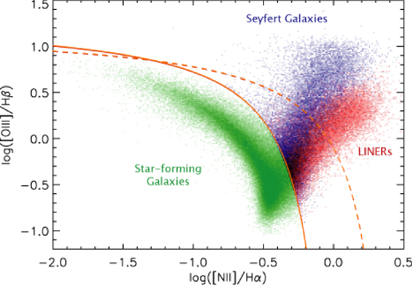
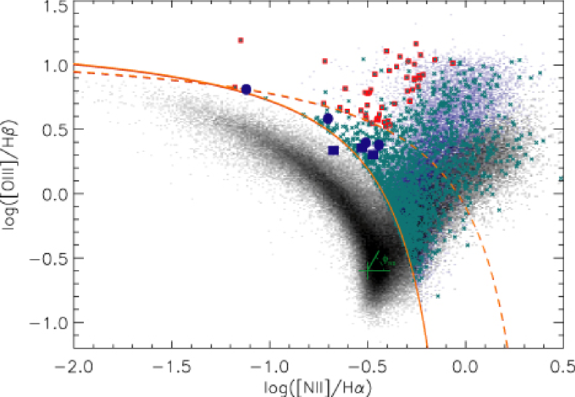
Figure 1 shows one of the standard line ratio diagrams (Baldwin, Phillips, & Terlevich, 1981) used to distinguish star-forming galaxies, Seyfert 2 galaxies (or AGN NLRs) and Low Ionization Nuclear Emission-line Region galaxies (LINERs). A detailed description of the location of these different classes of object in the different line ratio diagrams and the criteria that define our classification system has been given in a recent paper by Kewley et al. (2006).

In this particular diagram, the emission line galaxies are distributed in $V$-shaped morphology, with the star-forming galaxies located in the left branch and the AGN in the right branch. The AGN branch actually consists of two classes of object, the Seyfert 2 galaxies and the LINERs (Kewley et al., 2006).

The distribution of the starforming galaxies along the horizontal [N ii]$\lambda 6584$Å/$\mbox{H}\alpha$ axis is strongly correlated with the metallicity within the starforming region and the mass of the galaxy; both increase with increasing [N ii]/$\mbox{H}\alpha$. The vertical axis of [O iii]$\lambda 5007$Å/$\mbox{H}\beta$ is associated with the average ionization state and temperature of the photoionized gas in the emission line galaxy. AGN are offset from the star-forming galaxies on this axis because of their much harder ionizing spectrum. Those objects which lie at the extremities of the AGN branch are “pure” AGN. As the contribution of star-formation to the emission line spectrum increases, the strength of [O iii]/$\mbox{H}\beta$ decreases. This AGN-starburst mixing sequence culminates at the fulcrum of the $V$, where starforming galaxies and AGN dominated by starformation become indistinguishable. When we model NLR spectra, we consider only “pure” AGN.

3 Low Metallicity NLR simulations

We have run a series of narrow line region (NLR) models with a wide range in both metallicity and ionization parameter. The models are based upon the dusty, radiation pressure dominated models of Groves et al. (2004a, b), but use a more realistic ionizing spectrum (Groves et al., 2006). While it is unknown whether low metallicity AGN will contain dust, the observations of dust in high-$z$ objects indicates that such an assumption is not unreasonable (Bertoldi et al., 2003). Unlike previous work on NLR metallicity (eg Storchi-Bergmann et al., 1998), these models assume a more physical structure for the NLR clouds and concentrate upon the effects of low metallicity.

As the models have been discussed in depth in previous papers, we only describe the relevant parameters and the changes that were made in order to address the issue of low metallicity AGN. Throughout this work we assume a fiducial value of $n_{\mathrm{H}}\sim 10^{3}$$\,\mbox{cm}^{-3}$ for the density as found in previous papers.

3.1 Metallicity and Dust Depletion

The assumed abundances are based upon the solar abundance set of Asplund et al. (2005), which takes into account recent revisions of the solar abundances of several important elements like carbon and oxygen. Note that abundance ratios may vary between different AGN and even within the NLR of a single AGN; the abundances given in table 1 are thus meant to be representative.

Table 1: Solar abundance & metallicity scaling

Element	Abundance	Depletion
H …………………………….	0.0000	0.000
He…………………………….	$-$0.9870	0.000
C …………………………….	$-$3.6100	$-$0.300
N …………………………….	$-$4.2000	$-$0.300
O …………………………….	$-$3.3100	$-$0.240
Ne…………………………….	$-$3.9200	0.000
Na…………………………….	$-$5.6800	$-$0.600
Mg……………………………	$-$4.4200	$-$1.150
Al…………………………….	$-$5.5100	$-$1.440
Si……………………………..	$-$4.4900	$-$0.890
S …………………………….	$-$4.8000	$-$0.340
Cl…………………………….	$-$6.7200	$-$0.300
Ar……………………………	$-$5.6000	0.000
Ca……………………………	$-$5.6500	$-$2.520
Fe…………………………….	$-$4.5400	$-$1.370
Ni…………………………….	$-$5.7500	$-$1.400

As discussed in Groves et al. (2004a), the abundance with respect to hydrogen of most of the elements listed in table 1 will scale linearly with total metallicity. The exceptions are He and N. For helium, the yield from stars must be added to the primordial abundance. In this work, we use the primordial measurements of Pagel et al. (1992), which gives

$${\rm He}/{\rm H}=0.0737+0.0293Z/Z_{\odot}.$$ (1)

As nitrogen possesses both primary and secondary nucleosynthesis components, the relationship between nitrogen abundance and metallicity differs from that of other elements. For low metallicity galaxies (log (O/H) $\mathrel{\mathchoice{\lower 2.45pt\vbox{\halign{$\m@th\displaystyle\hfil#\hfil$\cr<\crcr\sim\crcr}}}{\lower 2.45pt\vbox{\halign{$\m@th\textstyle\hfil#\hfil$\cr<\crcr\sim\crcr}}}{\lower 2.45pt\vbox{\halign{$\m@th\scriptstyle\hfil#\hfil$\cr<\crcr\sim\crcr}}}{\lower 2.45pt\vbox{\halign{$\m@th\scriptscriptstyle\hfil#\hfil$\cr<\crcr\sim\crcr}}}}-4.0$) the N/O ratio is approximately constant, as expected for a “primary” element whose production is independent of metallicity. However, for higher metallicity galaxies (log (O/H) $\mathrel{\mathchoice{\lower 2.45pt\vbox{\halign{$\m@th\displaystyle\hfil#\hfil$\cr>\crcr\sim\crcr}}}{\lower 2.45pt\vbox{\halign{$\m@th\textstyle\hfil#\hfil$\cr>\crcr\sim\crcr}}}{\lower 2.45pt\vbox{\halign{$\m@th\scriptstyle\hfil#\hfil$\cr>\crcr\sim\crcr}}}{\lower 2.45pt\vbox{\halign{$\m@th\scriptscriptstyle\hfil#\hfil$\cr>\crcr\sim\crcr}}}}-3.5$) the N/O ratio is found to rise steeply with metallicity. This suggests that nitrogen becomes dominated by secondary production from CNO nucleosynthesis.

We follow Groves et al. (2004a) and use a linear combination of the primary and secondary components of Nitrogen. This relationship is fitted to the data from Mouhcine & Contini (2002) and Kennicutt, Bresolin, & Garnett (2003), with the requirement of matching the solar abundance patterns (see figure 2 in Groves et al., 2004a). With the new abundances in table 1 we obtain the following relation,

$$\left(\mathrm{N}/\mathrm{H}\right)=\left(\mathrm{O}/\mathrm{H}\right)\left(10^{-1.6}+10^{\left(2.37+\log_{10}\left[\mathrm{O}/\mathrm{H}\right]\right)}\right)$$ (2)

Using these prescriptions, we have then explored six NLR metallicities: $4Z_{\odot}$, $2Z_{\odot}$, $1Z_{\odot}$, $0.5Z_{\odot}$, $0.25Z_{\odot}$, $0.1Z_{\odot}$, and $0.05Z_{\odot}$. This range is wide enough to explore trends in emission line properties associated with a decrease in AGN metallicity. In terms of $12+\log($O/H$)$, these abundances correspond to 9.29, 8.99, 8.69, 8.39, 8.09, 7.69 and 7.39 respectively. Note that with the new Asplund et al. (2005) abundances, the oxygen abundance at solar is approximately 0.2 dex lower than that given in previous work (Grevesse & Sauval, 1998). As some of the metals present in the NLR clouds are depleted onto dust, the actual metallicity of the gas component in our models is approximately half of the total metallicity.

3.2 Narrow Line Region Dust

While the total dust to gas ratio is known to decrease with decreasing metallicity, the actual variation of dust abundance with metallicity is uncertain. In AGN no direct measurements can be made of dust depletion so for simplicity, we assume a solar depletion pattern for the dust and one that is constant with metallicity. In Galactic regions with different physical conditions, the dust to gas ratio, and hence the depletion factors, are observed to vary (Savage & Sembach, 1996). However, when regions of differing metallicities are observed, the depletion factors appear to be approximately constant (Vladilo, 2002). Our use of constant depletion factors for NLR models of differing metallicities is therefore not unreasonable.

The depletion factors, given in table 1, are based upon the recent work of Kimura et al. (2003) who examined the metal absorption along several lines of sight within the local bubble. The gas abundances were compared with solar abundances to determine the depletion. Some elements were not discussed in this work and for these we use previously assumed values from Dopita et al. (2000). For all other dust properties we follow the Groves et al. (2006) description of NLR dust. Note that any variation of the depletion factors will have a similar effect on the model to abundance variations.

3.3 Ionizing Spectrum

We follow Groves et al. (2006) and use an empirical fit to the Elvis et al. (1994) observations,

$$\begin{array}[]{rcl}f_{\nu}&=&\nu^{\alpha_{\mathrm{EUV}}}\exp\left(-\frac{h\nu}{kT_{\mathrm{UV}}}\right)\exp\left(-\frac{kT_{\mathrm{BBB}}}{h\nu}\right)\\ &+&a\nu^{\alpha_{\mathrm{X}}}\exp\left(-\frac{h\nu}{kT_{\mathrm{X}}}\right)\exp\left(-\frac{kT_{\mathrm{BBB}}}{h\nu}\right).\end{array}$$ (3)

with $\alpha_{\mathrm{EUV}}=-1.75$, $kT_{\mathrm{UV}}=120$ eV, $kT_{\mathrm{BBB}}=7.0$ eV.

The X-ray part of the spectrum has an index of $\alpha_{\mathrm{X}}=-0.85$ and an upper cut-off of $kT_{\mathrm{X}}=10^{5}$ eV. The parameter $a$ is set to $a=0.0055$, which results in an optical-X-ray slope of index $\alpha_{\mathrm{O-X}}\sim-1.4$. For simplicity, we use the same ionizing spectrum for AGN of all metallicities, but we note that a lower abundance of metals and especially dust is likely to alter the structure of the AGN torus and possibly even the accretion disk.

3.4 NLR model Parameters

For each metallicity we model a range of NLR ionization conditions. We follow the work of Groves et al. (2006) and maintain a constant total pressure across the models, while varying both the incident flux density and initial gas pressure. The total pressure we consider is $P_{\rm tot}/k=10^{7}$K$\,\mbox{cm}^{-3}$. This corresponds to a [S ii] density of $n_{\rm H}\simeq 10^{3}$$\,\mbox{cm}^{-3}$ which is a reasonable estimate of the NLR number density. While the effect of radiation pressure upon dust becomes less important at low metallicities, we maintain the same input parameters across the models for comparison purposes.

In table 2 we describe the parameters used for the model sets, with the same inputs used for each metallicity. For each input flux density and initial gas pressure we give the resulting initial ionization state in terms of two parameters, $\Xi_{0}$ and $\tilde{U}_{0}$ (Groves et al., 2006). $\Xi_{0}$ is a measure of the radiation pressure versus gas pressure ($\Xi_{0}=I_{0}/(cP_{gas})$), while $\tilde{U}_{0}$ measures the relative number of ionizing photons $S_{*}$, to a normalized initial density ($\tilde{U}_{0}=S_{*}/(c\tilde{n}_{\rm H})$, $\tilde{n}_{\rm H}=P_{\rm gas}/(k10^{4})$).

The parameters explored here span the range in ionization conditions that are observed in typical narrow line region clouds. The models are all truncated at a column density of $\log(N$(H i)$)=21$, which is reasonable for NLR clouds (e.g. Crenshaw et al., 2003).

Table 2: Input parameters for the models. The total incident flux density $I_{0}$ is scaled by $38.098$$\,\mbox{erg}\,\mbox{cm}^{-2}\mbox{s}^{-1}$, while $P_{0{\rm gas}}/k$ is scaled by $10^{6}$K$\,\mbox{cm}^{-3}$.

$model\#$	$I_{0}$	$P_{0{\rm gas}}/k$	$\Xi_{0}$	$\log(\tilde{U}_{0})$
1	4.0	1.00	20.16	-0.40
2	3.0	3.20	04.73	-1.03
3	2.0	5.40	01.87	-1.43
4	1.0	7.60	00.66	-1.88
5	0.5	8.70	00.29	-2.24
6	0.25	9.25	00.14	-2.57
7	0.1	9.58	00.05	-2.98

4 Metallicity Effects on the Emission Lines

When the total metallicity of a photoionized nebula decreases, there are several effects that cause changes in the final emission line spectrum. Many of these effects have been described elsewhere (eg Osterbrock, 1989; Dopita & Sutherland, 2003; Kewley & Dopita, 2002).

The dominant effect is the decreased abundance of an emitting species relative to hydrogen. This leads to weaker emission in lines such as nitrogen and oxygen relative to hydrogen recombination lines such as H$\alpha$ and H$\beta$. The line ratios relative to the other abundant primordial element, helium, also change in a similar way. This effect is not as strong, because helium also decreases with metallicity.

At metallicities above $0.1Z_{\odot}$, nitrogen is dominated by its secondary component. A decrease in metallicity down to this value results in a decrease of the strength of the nitrogen emission line relative to that of other metals. Below $Z\sim 0.1Z_{\odot}$, the primary component is dominant and the nitrogen tracks the behaviour of the other metal lines more closely. These trends are clearly seen in figure 2, which presents the models on the classic Baldwin, Phillips, & Terlevich (1981) (BPT) diagram of [N ii]$\lambda 6584$Å/$\mbox{H}\alpha$ versus [O iii]$\lambda 5007$Å/$\mbox{H}\beta$. This diagram clearly reveals the strong decrease of the nitrogen emission lines relative to hydrogen as the metallicity decreases.

Figure 2: The BPT diagram of [N ii]/$\mbox{H}\alpha$ versus [O iii]/$\mbox{H}\beta$ demonstrating the decrease of metal emission lines relative to hydrogen. This decrease is stronger for the nitrogen lines due to the secondary component in this element. Model metallicities are as labelled, with the small numbers next to model indicating model run and associated ionization parameter as given in table 2. The background image shows the log scale density distribution of the SDSS emission line sample, with Seyfert galaxies lying in the right, blue colored branch. Each branch has been scaled separately to emphasize the position of the Seyfert galaxies.

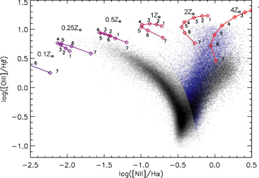
As metallicity decreases, the temperature of the nebula also increases. This is a result of the decrease in the efficiently cooling metal emission lines and the availability of more high energy photons to ionize hydrogen (see Sutherland & Dopita, 1993, for detailed explanations). Higher nebular temperatures affect the strength of temperature sensitive emission lines, such as [O iii]$\lambda 5007$Å, which increases with temperature. Line ratios like [O iii]$\lambda 5007$Å/$\mbox{H}\beta$ will thus decrease at a relatively slower rate with metallicity. This is also clear from the model presented in Figure 2. While temperature sensitive line ratios change with the metallicity of the gas, they are also strongly affected by the ionization state of the gas. This means that shocks and the varying contribution of star formation and AGN to the ionization become important.

Another effect of lowering the metallicity is that the opacity of the gas is reduced, meaning a greater volume is needed to absorb all ionizing photons. In AGN this effect causes noticeable differences because of the stronger contribution to the ionizing flux from X-rays, for which the hydrogen opacity is small. These X-rays give rise to the partially ionized region in NLRs, where important optical emission lines such as [O i]6300Å and [S ii]6713+31Å are emitted. Models with lower metallicity have larger partially ionized regions relative to the fully ionized region (see Groves et al., 2004a). In our column density limited models, the partially ionized region becomes truncated at low metallicities. As a result, we are not confident in our ability to use these models to calibrate some of the metallicity sensitive ratios commonly used in determining the abundances in star-forming galaxies, such as [N ii]/[S ii] and [S ii]/$\mbox{H}\alpha$ for use in the determination of AGN abundances.

5 Diagnostic Diagrams for Low Metallicity AGN

Generally, individual AGN are best reproduced with a combination of models, varying not only the metallicity, but also the ionizing spectrum, the density, the incident flux or ionization parameter and even the geometry (see eg Oliva et al., 1999).

However when looking at large numbers of AGN the best method is to look for trends or possible relationships between the line ratios and metallicity (eg Storchi-Bergmann et al., 1998; Nagao et al., 2002; Groves et al., 2004b). Previous AGN modelling has found that AGN as a group are best fit with models of around $2-4Z_{\odot}$, or $12+\log($O/H$)\sim 9.0-9.3$. Thus any AGN NLR found to have metallicities below solar could possibly be considered “low metallicity”.

As discussed in the previous section, line ratios relative to hydrogen are good diagnostics for low metallicity AGN. This is especially true for nitrogen with its secondary component as shown in figure 2. The diagnostic of [N ii]$\lambda 6584$Å/$\mbox{H}\alpha$ has been used as one of the main metallicity indicators in AGN due to its sensitivity and the strength of the lines (Storchi Bergmann & Pastoriza, 1989; Storchi-Bergmann et al., 1998). In general, low metallicity AGN will lie to the left of the Seyfert branch on the N ii BPT diagram. The decrease in the [O iii]/$\mbox{H}\beta$ ratio is not as strong because of the temperature sensitivity of this ratio.

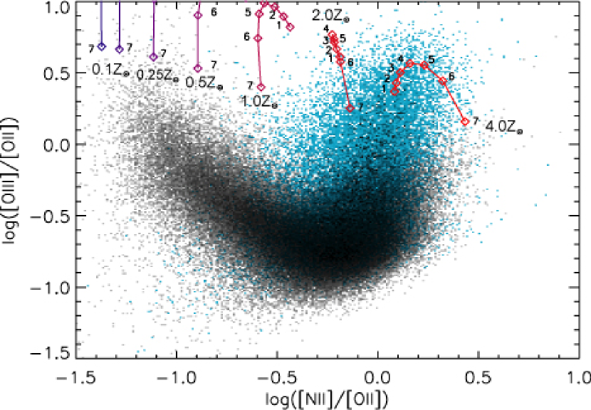
Another possible diagram for metallicity diagnosis is the [N ii]$\lambda 6584$Å/[O ii]$\lambda 3727$Å versus [O iii]$\lambda 5007$Å/ [O ii]$\lambda 3727$Å diagram, shown in figure 3. This again relies upon nitrogen to separate the different metallicities, but also uses the temperature sensitive ratio [O iii]/[O ii] as a secondary diagnostic. The [N ii]/[O ii] ratio will separate AGN with lower N ii relative to O ii. As N ii and O ii are both low ionization species , the ratio will only be weakly affected by the ionization or density conditions. In addition, star bursts and AGN have similar [N ii]/[O ii] ratios for similar metallicities, so the abundance determination of an active galaxy is only slightly perturbed by any contribution from star formation. The main disadvantage of this ratio is that [N ii] and [O ii] are widely separated in wavelength and the ratio is hence much more sensitive to the effects of reddening. The [O iii]/[O ii] ratio is similar to [O iii]/$\mbox{H}\beta$ as a temperature sensitive diagnostic in that is good in separating the Seyferts from the star-forming galaxies. It also has the additional benefit of not being strongly sensitive to metallicity.

Figure 3: Metallicity diagnostic diagram of [N ii]$\lambda 6584$Å/[O ii]$\lambda 3727$Å versus [O iii]$\lambda 5007$Å/ [O ii]$\lambda 3727$Å with models increasing in metallicity from left to right (as labelled). The background image shows the distribution of the SDSS emission line galaxies, with Seyfert galaxies, colored blue, lying in the vertical branch and starbursts in the horizontal branch. Each branch has been scaled separately to emphasize the position of the Seyfert galaxies. The contribution by star formation to the AGN decreases the [O iii]/[O ii] ratio.

Both these diagnostic diagrams rely heavily on the [N ii] line to estimate the metallicity. This means that the diagnostic is sensitive to abundance variations relative to solar within the NLR due to differing star formation histories.

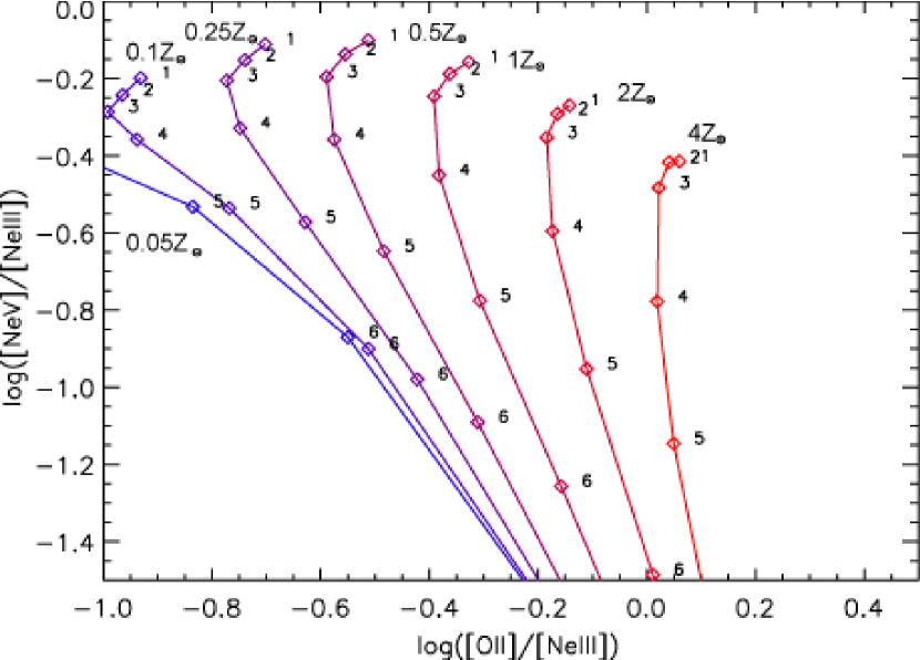
At higher redshift, the [N ii] line is no longer observable, but UV diagnostics become useful (Nagao et al., 2006; Groves et al., 2004b). One possible diagram is shown in figure 4, which plots the Near–UV line ratios of [O ii]$\lambda 3727,9$Å /[Ne iii]$\lambda 3869$Å versus [Ne v]$\lambda 3426$Å/[Ne iii]$\lambda 3869$Å. This diagram relies upon the temperature sensitivity of the [Ne iii] line to distinguish different metallicities in the [O ii]/[Ne iii] ratio. The [Ne v]/[Ne iii] ratio, while weakly dependent upon metallicity, is very sensitive to the ionizing spectrum and ionization state of the gas. Thus this ratio provides a way of distinguishing star-forming galaxies, which have very little [Ne v] emission, from AGN. As in figure 3, the strength of figure 4 lies in its use of strong lines and its ability to distinguish star forming galaxies from AGN.

Figure 4: Near–UV metallicity diagnostic diagram of [O ii]$\lambda 3727,9$Å/[Ne iii]$\lambda 3869$Å versus [Ne v]$\lambda 3426$Å/[Ne iii]$\lambda 3869$Å. Pure star forming galaxies would lie below these curves at low [Ne v]/[Ne iii] values.

6 AGN Selection within SDSS

Within this work we use the SDSS Data Release 4 (DR4) spectroscopic galaxy sample (Adelman-McCarthy et al., 2006), which includes $u$-, $g$-, $r$-, $i$- and $z$-band photometry and spectroscopy of over 500,000 objects. The spectra are taken using 3-arcsec diameter fibres, positioned as close as possible to the centres of the target galaxies. The flux- and wavelength-calibrated spectra cover the range from 3800 to 9200Å, with a resolution of $R\sim$1800.

At the median redshift of the sample ($z\sim 0.1$) the spectroscopic fibre typically contains 20 to 40 percent of the total galaxy light, thus contain a component due to the host galaxy as well as the AGN. As described in Tremonti et al. (2004), we subtract the contribution of the stellar continuum from each spectrum, using the best fitting combination of template spectra from the population synthesis code of Bruzual & Charlot (2003). The best-fitting model also places constraints on the star formation history and metallicity of the galaxy(Gallazzi et al., 2005), and can be used to estimate stellar masses and star-formation histories (Kauffmann et al., 2003a).

We have used the same sample criteria as in Kewley et al. (2006) to extract our narrow-line AGN subsample. The sample is limited to redshifts above 0.02. We also apply a signal-to-noise cut ($S/N>3$) on the six dominant emission lines; $\mbox{H}\beta$ $\lambda 4861$Å, [O iii] $\lambda 5007$Å, [O i] $\lambda 6300$Å, $\mbox{H}\alpha$ $\lambda 6563$Å, [N ii] $\lambda 6584$Å, and the doublet [S ii] $\lambda 6716,31$Å. This gives a sample of $\sim 170,000$ emission line galaxies. The Kauffmann et al. (2003c) N ii empirical relation is then used to define our AGN sample,

$$\log([\mathrm{OIII}]/\mathrm{H}\beta)>0.61/(\mathrm{NII}]/\mathrm{H}\alpha-0.05))+1.3.$$ (4)

This results in a sub-sample of $\sim 50000$ galaxies classified as AGN. The N ii dividing line of Kewley & Dopita (2002),

$$\log([\mathrm{OIII}]/\mathrm{H}\beta)>0.61/(\mathrm{NII}]/\mathrm{H}\alpha-0.47))+1.19,$$ (5)

is used to select a subsample of 20,000 “pure” AGN where the ionization is dominated by the active nucleus rather than H ii regions.

The AGN sample includes two classes of emission line objects; Seyfert 2s and Low Ionization Nuclear Emission-line Regions (LINERs). In this work we consider only Seyfert galaxies, as our diagnostic models for the NLR only apply to these objects. To distinguish LINERs from Seyferts, we use the recent empirical dividing lines from Kewley et al. (2006)

$$\log([\mathrm{OIII}]/\mathrm{H}\beta)>1.36\log([\mathrm{OI}]/\mathrm{H}\alpha)+1.4,$$ (6)

Our final sample consists of 8800 pure Seyfert galaxies ranging in redshift from $z\sim 0.02$ to $\sim 0.36$, with a median of $z\sim 0.1$.

6.1 Accounting for Reddening in the SDSS Sample

Line ratios such as [N ii]/[O ii] have a large separation in wavelength and thus need to be corrected for reddening. We use the $\mbox{H}\alpha$/$\mbox{H}\beta$ ratio and we assume dust-free values of 2.86 for star-forming galaxies and 3.1 for Seyferts. The majority of AGN in our sample will have ongoing starformation and their dust-free values of this ratio should lie between these values. We then assume the power-law slope of $\lambda^{-0.7}$ from Charlot & Fall (2000) to correct for the attenuation in each galaxy.

7 Low Metallicity AGN in SDSS

Measurements of the average gas metallicities in starforming galaxies (fig. 6, Tremonti et al., 2004) show that there is a strong trend of increasing metallicity with increasing stellar mass. This trend is also seen in the average stellar metallicities in normal galaxies (fig. 8, Gallazzi et al., 2005).

Figure 5: The Stellar Mass distribution of the full emission line galaxy sample (solid line) and the AGN (including LINER) dominated galaxies (dashed line) in Solar masses. The peaks have been scaled by 11013 and 2286 for the full and AGN sample respectively.

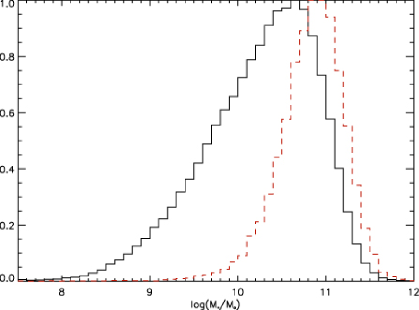
Figure 5 shows the mass distribution of the full emission-line galaxy sample and the AGN sample. AGN are clearly biased towards higher masses (Kauffmann et al., 2003c) and they range from $\sim 10^{10}$ to $\sim 10^{11.5}$M_⊙. If AGN have similar metallicities to star-forming galaxies, they should have abundances in the range $12+\log({\rm O/H})\sim 8.95$ to $\sim 9.13$ (Tremonti et al., 2004, eqn. 3), or metallicities of 2-3$Z_{\odot}$. As shown in figure 2 this is also the metallicity range for which our AGN photoionization models best reproduce the emission line ratios of the typical Seyfert galaxies within our sample.

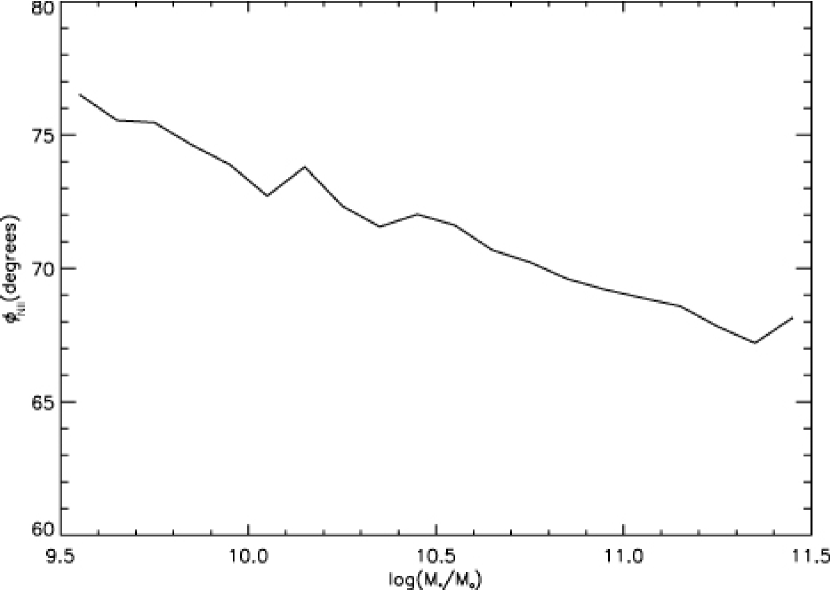
Figure 2 shows that as the metallicity decreases, AGN are expected to migrate to the left on the [O iii]/$\mbox{H}\beta$ versus [N ii]/$\mbox{H}\alpha$ BPT diagram. Following Kewley et al. (2006), we choose an empirical base point on the [N ii] BPT diagram ([-0.5,-0.6], as marked on figure 7) and use this as the vertex to determine the angle each AGN in our sample makes with the $x$-axis. We label this angle $\phi_{\mathrm{NII}}$. Figure 6 shows the variation of the median value of this angle as a function of the stellar mass of the host. This figure clearly reveals a correlation between the host stellar mass and metallicity. The change in $\phi_{NII}$ from $\log M_{*}\sim 9.5$ to $\log M_{*}\sim 11.5$ corresponds to a change of about 0.2 – 0.3 dex in log(O/H) in the AGN models.

Figure 6: Variation of the median angle of the Seyfert branch, $\phi_{NII}$, with the host stellar mass, $M_{*}$ in solar masses. $\phi_{\mathrm{NII}}$ is the angle relative to the $x$-axis on the BPT [N ii] diagram using the empirical point $[-0.5,-0.6]$ as the vertex (see figure 7). Only AGN-dominated Seyfert classified galaxies are considered.

We then use a cut in stellar mass to separate out a sample of low metallicity AGN for closer inspection. We select AGN hosts with log(M${}_{*}/\mathrm{M}_{\odot})<10.0$. This limit selects the tail end of the AGN mass distribution, while maintaining sufficient numbers for analysis. This yields 1800 low-mass AGN, of which 650 lie above the Kewley line. Figure 7 shows the distribution of the low-mass AGN (both Seyferts and LINERs) on the standard BPT [N ii] diagram. As can be seen, the low mass objects, while scattered, tend to lie towards the left of the AGN branch. Many of them are strongly clustered close to the Kauffmann dividing line. To reduce the effects of confusion and contamination by star-formation, we concentrate on the Seyfert galaxies that lie above the Kewley line. This reduces the sample to $\sim 350$ galaxies,

Figure 7: The BPT [N ii]/$\mbox{H}\alpha$ versus [O iii]/$\mbox{H}\beta$ diagram showing the distribution of the low mass AGN (crosses). The background image shows the log scale density distribution of the full SDSS emission line sample as in figure 2. The solid and dashed curves show the Kauffmann and Kewley classification lines respectively. The boxed crosses highlight the lowest metallicity low mass Seyfert galaxies (see figure 8). The solid squares and circles represent the Shapley et al. (2005) and Erb et al. (2006) high redshift star-forming galaxies respectively, and show their position relative to the low metallicity AGN. (see §8).

To estimate the metallicity of the low mass AGN we plot these objects in the [N ii]$\lambda 6584$Å/[O ii]$\lambda 3727$Å versus [O iii]$\lambda 5007$Å/[O ii]$\lambda 3727$Å diagram described in the previous section. This is shown in figure 8. The use of the Kewley cut means that the majority of starburst dominated AGN have been removed from the sample as can be seen from the scarcity of objects in the heavily shaded greyscale region. However there are still some objects which appear to lie in the starburst branch. These galaxies may either have incorrectly measured line fluxes or incorrect reddening corrections (as is certainly the case for the lowest [O iii]/[O ii] object). Once again the low mass Seyferts tend to lie to the left, low metallicity side of the main Seyfert branch.

Figure 8: The metallicity sensitive [N ii]$\lambda 6584$Å/[O ii]$\lambda 3727$Å versus [O iii]$\lambda 5007$Å/[O ii]$\lambda 3727$Å diagram showing the distribution of the low mass Kewley-selected AGN galaxies (crosses). The background image shows the logscale density distribution of the full SDSS emission line sample. The Seyfert galaxies, marked as blue on the image, lie on the vertical branch at high [N ii]/[O ii], while the star-forming galaxies lie on the mainly horizontal curve. LINERs exist at the dark clump on the star-forming branch at high [N ii]/[O ii]. The dotted lines indicate our arbitrary metal & AGN cuts, with our final low mass, low metallicity AGN highlighted by squares.

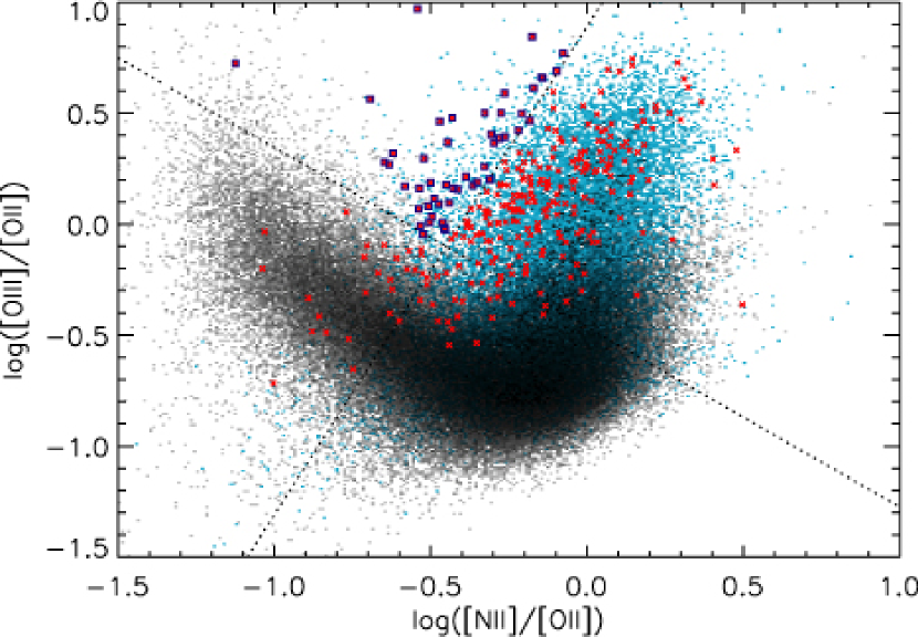
Figure 8 demonstrates is that even at the low mass end of the AGN distribution, the AGN gas metallicity is still around solar (accounting for dust depletion). We note that this is similar to the gas-phase metallicities of star-forming galaxies of the same mass (equation 3 in Tremonti et al., 2004).

To select the most extreme low metallicity AGN in our sample, we apply two cuts to exclude those objects that lie within the main AGN or starforming branches. These cuts are shown by the dotted lines in figure 8 and are:

$$\begin{array}[]{rcl}\log([\mathrm{OIII}]/[\mathrm{OII}])&\geq&2.1\log([\mathrm{NII}]/[\mathrm{OII}])+0.85\\ \log([\mathrm{OIII}]/[\mathrm{OII}])&\geq&-1.2\log([\mathrm{NII}]/[\mathrm{OII}])-0.7.\end{array}$$ (7)

These cuts select 50 of the 559 low mass AGN as our lowest metallicity candidates, and they are plotted as boxed crosses on figures 7 and 8. Note that one object has multiple spectra, which leaves 47 unique candidates. Six of these objects lie at redshifts greater than 0.1, with at least one being a strongly starbursting galaxy. These low “metallicity” AGN lie clearly to the left of the AGN branch in the BPT [N ii] diagram (see figure 7), and similarly lie on the left part of the AGN branch in both the BPT [S ii] and [O i] diagrams. The few low mass AGN that lie to the left of the AGN branch on figure 7 and are not selected by our cuts are actually at too low a redshift ($z\mathrel{\mathchoice{\lower 2.45pt\vbox{\halign{$\m@th\displaystyle\hfil#\hfil$\cr<\crcr\sim\crcr}}}{\lower 2.45pt\vbox{\halign{$\m@th\textstyle\hfil#\hfil$\cr<\crcr\sim\crcr}}}{\lower 2.45pt\vbox{\halign{$\m@th\scriptstyle\hfil#\hfil$\cr<\crcr\sim\crcr}}}{\lower 2.45pt\vbox{\halign{$\m@th\scriptscriptstyle\hfil#\hfil$\cr<\crcr\sim\crcr}}}}0.03$) for accurate measurement of the [O ii] line flux.

Figure 9: SDSS fibre spectra of six of the low mass, low metallicity selected AGN. a) shows the spectrum of a starburst galaxy that falls in our selection criteria while b) – f) shows five representative low metallicity AGN. The difference between the starburst and AGN can be seen, as well as other AGN signatures, such as the strong [He ii]$\lambda 4686$Å line (unmarked line to the left of $\mbox{H}\beta$), or old stellar continuum.

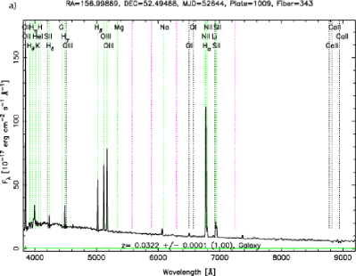
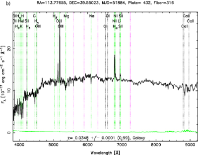
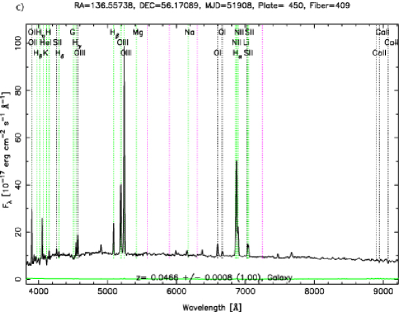
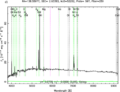
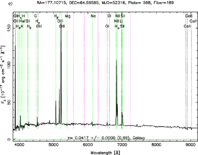
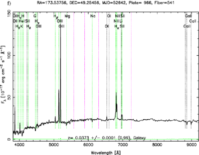
As a final check we examined the spectra of these objects and a representative selection of these is shown in figure 9. One of these objects (figure 9a), the galaxy with the lowest [N ii]/[O ii] ratio, is a clear starforming galaxy with an apparent incorrectly estimated [O iii]5007 strength. However this is the only clear pure starburst galaxy among the 41 objects. Some of the spectra of the other 40 AGN candidates exhibit clear signatures of young stars as well as He ii $\lambda 4686$Å emission. Others are dominated by older stars, and there are also a number of AGN with strong Balmer absorption lines. All objects have very weak [N ii]6584 and [O i]6300 (expected because of their low metallicities), but the strong [O iii]5007 emission line and relatively strong [S ii] 6716,31 doublet classify these objects as AGN. One other point to note is the presence of the [O iii]$\lambda 4363$Å line in many of the spectra, indicative of the high gas temperatures in these objects, and also suggestive of low metallicities.

Figure 10: SDSS images of the six sample galaxies from figure 9 with a) an example starburst galaxy and b) – f) low mass AGN. Each image shows the same area, with the bar in each frame indicating 5″. The image centre, as marked by the lines, is the position of the 3″ SDSS fibre centre. Note that for most AGN the 3″ fibre encompasses a significant fraction of the host galaxy.

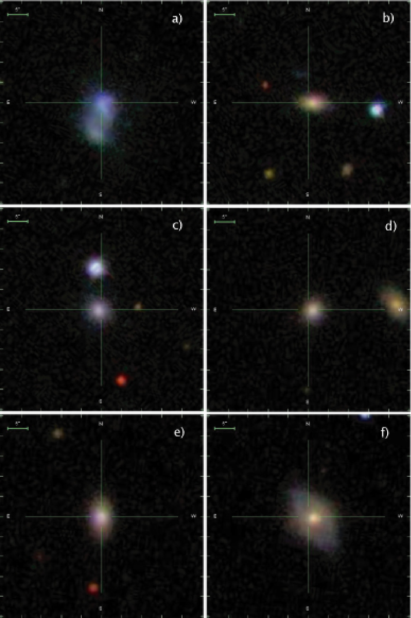
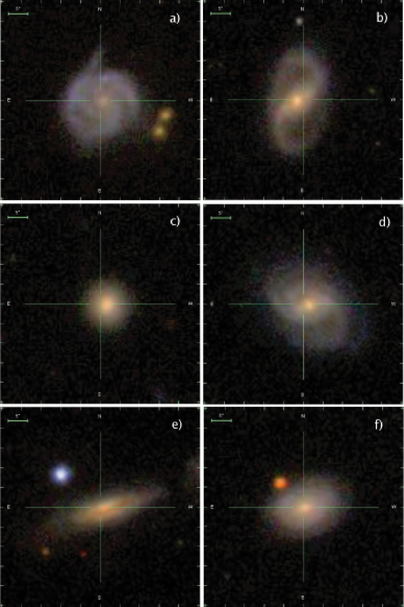
As a complement to the SDSS fibre spectra, we also show images of the same sample in figure 10. The starforming galaxy has a distinctly different morphology compared to the AGN, appearing diffuse and blue in color. The images of the low mass AGN indicate that their host galaxies are faint and relatively compact. They tend to be red, with a disky or lenticular structure surrounding a relatively bright nucleus. For comparison, in figure 11 we show Seyfert galaxies that fall in the main branch on line diagnostic diagrams and have a median redshift similar to the low mass sample of $z\sim 0.05$. The most obvious difference is their size. The spiral structure in the host galaxy is also much more evident. However in some respects the low mass and high mass AGN are similar; both have a bright red nucleus/bulge, and diffuse, blue outer disk.

Figure 11: SDSS images of six random NLR dominated Seyfert galaxies. These galaxies have redshifts $z=0.05\pm 0.01$, and all fall within the main Seyfert branch on line diagnostic diagrams. Markings the same as in figure 10.

7.1 The Lowest Metallicity AGN

In the previous section, we searched for low metallicity AGN by looking for objects offset from the main AGN branch. However the diagnostic diagrams of section 5 indicate that the lowest metallicity objects could actually lie within or even below the star-forming branch.

To explore this possibility, we selected from the SDSS sample all objects with a signal-to-noise greater than 3 in $\mbox{H}\alpha$, $\mbox{H}\beta$ and [O iii]$\lambda 5007$Å, and looked at the metallicity sensitive line ratios such as [S ii]/$\mbox{H}\alpha$  [Ne iii]/$\mbox{H}\beta$ or [N ii]/[O ii]. The spectra, images and galaxy parameters of all objects with extremely low values of these ratios were examined.

All of these objects appeared to be indistinguishable from low mass, low metallicity starburst galaxies. They all had blue colours and high equivalent width emission lines. None showed obvious signs of AGN activity, such as the He ii $\lambda 4686$Å emission line or [Ne v]$\lambda 3426$Å emission in the higher redshift objects. We found no clear evidence for extremely low metallicity AGN. If such objects exist, they are either very rare they are indistinguishable from a low metallicity starburst galaxy.

8 Discussion

Low metallicity AGN appear to be very rare objects, at least locally. The SDSS emission line galaxy sample only gives approximately 40 AGN with a mass below $10^{10}\mathrm{M}_{\odot}$ and a significant detectable difference in their abundances relative to typical Seyfert galaxies.

The use of a low mass selection criterion is supported by the observations which reveal a correlation between mass and metal sensitive line ratios such as [N ii]/$\mbox{H}\alpha$. An exact determination of a mass–metallicity relationship in AGN is hindered by the difficulty of measuring with any accuracy the metallicity in the AGN hosts.

The 40 low metallicity AGN selected out of the 23000 Seyfert 2s in our original SDSS sample appear to have metallicities around half that of typical AGN. This leads to two questions: where are the low metallicity AGN and why are there no AGN with even lower metallicities?

We do lose some objects because we use the [O ii]$\lambda 3626$Å line as a diagnostic, which means we miss low metallicity objects below $z\sim 0.03$. Approximately 50 low mass AGN lie below this redshift, but we estimate that only 10 would fall into the low metallicity category. Another possibility is that low metallicity AGN are “hidden” by strong star formation. As discussed in Kauffmann et al. (2003b), a large fraction of low mass galaxies are experiencing bursts of starformation and show strong line emission. However figure 6 in Kauffmann et al. (2003c) demonstrates that it is not easy to hide a typical AGN of high metallicity. These authors added AGN of different [O iii] luminosities to low mass starburst galaxies and showed that at [O iii] luminosities above $10^{6}L_{\odot}$, all of them would have been detected. We have repeated the same analysis for low metallicity AGN and we find very similar results.

It is thus clear that low metallicity AGN are rare in the local Universe, What about at high redshift? Our emission-line diagnostics involve the rest-frame optical band, and the required spectroscopy is challenging at high redshift. Nevertheless, Shapley et al. (2005) and Erb et al. (2006) have recently measured the $\mbox{H}\beta$, [O iii]$\lambda$5007, $\mbox{H}\alpha$, and [N ii]$\lambda$6584 emission line fluxes in two small samples of galaxies at $z\sim$ 1.4 and $z\sim 2.3$ respectively. We have plotted the locations of these galaxies in Figure 7. Nearly all the objects lie between the Kauffmann and Kewley classification lines. This region is dominated by composite objects, where both an AGN and star formation contribute significantly to the emission-lines. However, the high redshift galaxies are displaced to significantly lower [N ii]/$\mbox{H}\alpha$ratios than typical SDSS composite galaxies.

The most natural interpretation of this is that these high redshift galaxies are indeed composite galaxies, but of lower metallicity than the typical SDSS galaxies. Similar objects comprise only a small fraction of the SDSS sample, but in the region where most of the high redshift galaxies are located, bounded by the two classification curves and the main Seyfert branch ($\log([$O iii$]/$$\mbox{H}\beta$$)\mathrel{\mathchoice{\lower 2.45pt\vbox{\halign{$\m@th\displaystyle\hfil#\hfil$\cr>\crcr\sim\crcr}}}{\lower 2.45pt\vbox{\halign{$\m@th\textstyle\hfil#\hfil$\cr>\crcr\sim\crcr}}}{\lower 2.45pt\vbox{\halign{$\m@th\scriptstyle\hfil#\hfil$\cr>\crcr\sim\crcr}}}{\lower 2.45pt\vbox{\halign{$\m@th\scriptscriptstyle\hfil#\hfil$\cr>\crcr\sim\crcr}}}}3\log([$N ii$]/$$\mbox{H}\alpha$$)$), we still find about 500 SDSS galaxies. Modelling these as composites implies that the AGN would produce 50 to 70% of the [O iii]5007 flux, but only about 20% of the $\mbox{H}\alpha$ and $\mbox{H}\beta$ flux. A definitive test of the presence of an AGN would require the detection of the He ii$\lambda$4686 or [Ne v]$\lambda$3426 lines. Unfortunately, the former line is expected to be weak (a 20% AGN contribution to H$\beta$ implies He ii/$\mbox{H}\beta$= 0.05), while the latter line is not redshifted into the SDSS spectral band for the great majority of objects.

While we can not definitively say that typical SDSS galaxies with spectra similar to the high redshift galaxies have AGN, there are indirect pieces of evidence that strongly suggest that this is the case. When compared with a sample of nearby pure star-forming galaxies (all galaxies within $\pm 0.05$ dex of [-0.55,0.10] on the N ii BPT diagram), we find that the host galaxies of these candidate low-metallicity composites differ in a way that is similar to what is found for the host galaxies of AGN (Kauffmann et al., 2003c; Heckman et al., 2004). They have on average significantly higher stellar masses ($\sim 0.3$ dex), older stellar populations (D4000 of 1.29 compared to 1.16), redder colors ($\sim 0.2$ greater in $g-r$) and weaker $\mbox{H}\alpha$ equivalent widths than the pure star forming galaxies. Similar differences are found in their surface mass density, $\sigma_{*}$, Concentration index and other galactic parameters. A comparison of the composites with objects just below the Kauffmann classification curve shows similar, albeit weaker, differences. However within the composite region there are some galaxies that are likely to be pure starforming galaxies as they have strong $\mbox{H}\alpha$ equivalent widths and host properties that are similar to ordinary star-forming galaxies.

The Erb et al. (2006) object at $\log($[N ii]/$\mbox{H}\alpha$$)\approx-1.0$ is the clear exception to the previous objects. Lying above both the Kauffmann and Kewley classification curves, it requires a much greater contribution by an AGN to be offset from the star-forming branch due to its low metallicity.In our SDSS AGN selected sample, we have no low metallicity AGN or composites with which to compare this object. If we select the few SDSS objects that lie within the errors of the Erb object, all are clear starbursting galaxies with indicators such as the neon emission lines and He ii$\lambda 4686$Å are so weak, if present at all, as to indicate that the contribution of an AGN to the spectrum is negligible. Thus this object is most likely to be a low metallicity starburst.

We conclude that most of the high redshift galaxies in Figure 7 are most likely to be composite objects with an AGN. Fortunately, the AGN will have only a modest effect on the [N ii]/$\mbox{H}\alpha$ ratio used by Shapley et al. (2005) and Erb et al. (2006) to measure the metallicity. We estimate that the AGN contribution will increase [N ii]/$\mbox{H}\alpha$ by only about 0.1 to 0.2 dex, and hence cause the metallicity to be overestimated by less than 0.1 dex (Pettini & Pagel, 2004).

If the Shapley et al. (2005) and Erb et al. (2006) galaxies are composite AGN/starforming galaxies, this may imply that low metallicity AGN are more common at high redshifts. We note, however, that investigations of the metallicities of QSOs at redshifts greater than 1 using both broad and narrow emission lines all appear to show solar to supersolar metallicities (e.g. Dietrich et al., 2003; Nagao et al., 2006).

The scarcity of low metallicity AGN locally is very suggestive. The results indicate that it is unlikely for a strong AGN to be found in a galaxy whose mass is less than $\sim 10^{10}\mathrm{M}_{\odot}$, or whose metallicity is less than solar. It is not clear whether this indicates that black holes only form in galaxies above some mass threshhold. There is considerable evidence that high luminosity AGN are hosted by galaxies with young stellar populations and strong post-burst features (Kauffmann et al., 2003c). This suggests that the AGN must be preceded by strong star formation and this may also explain the high metallicities in the NLR gas. Further studies of AGN in low mass hosts (see e.g. Greene & Ho, 2004), and at early cosmological epochs when the mean star formation rate and gas densities were much higher will shed more light on these questions.

References

- Adelman-McCarthy et al. (2006) Adelman-McCarthy, J. K., et al. 2006, ApJS, 162, 38
- Aller (1942) Aller, L. H. 1942, ApJ, 95, 52
- Asplund et al. (2005) Asplund, M., Grevesse, N., & Sauval, A. J. 2005, ASP Conf. Ser. 336: Cosmic Abundances as Records of Stellar Evolution and Nucleosynthesis, 336, 25
- Baldwin, Phillips, & Terlevich (1981) Baldwin, J. A., Phillips, M. M., & Terlevich, R. 1981, PASP, 93, 5 (BPT)
- Baldwin et al. (1995) Baldwin, J., Ferland, G., Korista, K., & Verner, D. 1995, ApJ, 455, L119
- Barth et al. (2005) Barth, A. J., Greene, J. E., & Ho, L. C. 2005, ApJ, 619, L151
- Bertoldi et al. (2003) Bertoldi, F., Carilli, C. L., Cox, P., Fan, X., Strauss, M. A., Beelen, A., Omont, A., & Zylka, R. 2003, A&A, 406, L55
- Bruzual & Charlot (2003) Bruzual, G., & Charlot, S. 2003, MNRAS, 344, 1000
- Charlot & Longhetti (2001) Charlot, S., & Longhetti, M. 2001, MNRAS, 323, 887
- Charlot & Fall (2000) Charlot, S., & Fall, S. M. 2000, ApJ, 539, 718
- Cid Fernandes et al. (2001) Cid Fernandes, R., Heckman, T., Schmitt, H., Delgado, R. M. G., & Storchi-Bergmann, T. 2001, ApJ, 558, 81
- Cid Fernandes et al. (2004) Cid Fernandes, R., Gu, Q., Melnick, J., Terlevich, E., Terlevich, R., Kunth, D., Rodrigues Lacerda, R., & Joguet, B. 2004, MNRAS, 355, 273
- Crenshaw et al. (2003) Crenshaw, D. M., Kraemer, S. B., & George, I. M. 2003, ARA&A, 41, 117
- Davidson & Netzer (1979) Davidson, K., & Netzer, H. 1979, Reviews of Modern Physics, 51, 715
- Dietrich et al. (2003) Dietrich, M., Hamann, F., Shields, J. C., Constantin, A., Heidt, J., Jäger, K., Vestergaard, M., & Wagner, S. J. 2003, ApJ, 589, 722
- Dopita et al. (2000) Dopita, M. A., Kewley, L. J., Heisler, C. A., & Sutherland, R. S. 2000, ApJ, 542, 224
- Dopita & Sutherland (2003) Dopita, M. A., & Sutherland, R. S. 2003, Astrophysics of the diffuse universe, Berlin, New York: Springer, 2003. Astronomy and astrophysics library, ISBN 3540433627,
- Elvis et al. (1994) Elvis, M., et al. 1994, ApJS, 95, 1
- Erb et al. (2006) Erb, D. K., Shapley, A. E., Pettini, M., Steidel, C., Reddy, N., & Adelberger, K. 2006, ApJ, accepted (astro-ph/0602473)
- Ferrarese & Merritt (2000) Ferrarese, L., & Merritt, D. 2000, ApJ, 539, L9
- Gallazzi et al. (2005) Gallazzi, A., Charlot, S., Brinchmann, J., White, S. D. M., & Tremonti, C. A. 2005, MNRAS, 362, 41
- Gebhardt et al. (2000) Gebhardt, K., et al. 2000, ApJ, 539, L13
- Greene & Ho (2004) Greene, J. E., & Ho, L. C. 2004, ApJ, 610, 722
- Grevesse & Sauval (1998) Grevesse, N. & Sauval, A. J. 1998, Space Science Reviews, 85, 161
- Groves et al. (2004a) Groves, B. A., Dopita, M. A., & Sutherland, R. S. 2004, ApJS, 153, 9
- Groves et al. (2004b) Groves, B. A., Dopita, M. A., & Sutherland, R. S. 2004, ApJS, 153, 75
- Groves et al. (2006) Groves, B. A., Dopita, M. A., & Sutherland, R. S. 2006, in prep.
- Haehnelt et al. (1998) Haehnelt, M. G., Natarajan, P., & Rees, M. J. 1998, MNRAS, 300, 817
- Hamann & Ferland (1993) Hamann, F., & Ferland, G. 1993, ApJ, 418, 11
- Hamann & Ferland (1999) Hamann, F., & Ferland, G. 1999, ARA&A, 37, 487
- Hamann et al. (2002) Hamann, F., Korista, K. T., Ferland, G. J., Warner, C., & Baldwin, J. 2002, ApJ, 564, 592
- Heckman et al. (2004) Heckman, T. M., Kauffmann, G., Brinchmann, J., Charlot, S., Tremonti, C., & White, S. D. M. 2004, ApJ, 613, 109
- Kauffmann & Haehnelt (2000) Kauffmann, G., & Haehnelt, M. 2000, MNRAS, 311, 576
- Kauffmann et al. (2003a) Kauffmann, G., et al. 2003, MNRAS, 341, 33
- Kauffmann et al. (2003b) Kauffmann, G., et al. 2003, MNRAS, 341, 54
- Kauffmann et al. (2003c) Kauffmann, G., et al. 2003, MNRAS, 346, 1055
- Kewley & Dopita (2002) Kewley, L. J., & Dopita, M. A. 2002, ApJS, 142, 35
- Kewley et al. (2006) Kewley, L., et al. 2006, in prep.
- Kimura et al. (2003) Kimura, H., Mann, I., & Jessberger, E. K. 2003, ApJ, 582, 846
- Kennicutt, Bresolin, & Garnett (2003) Kennicutt, R. C., Bresolin, F., & Garnett, D. R. 2003, ApJ, 591, 801
- Komossa & Schulz (1997) Komossa, S., & Schulz, H. 1997, A&A, 323, 31
- Kormendy & Richstone (1995) Kormendy, J., & Richstone, D. 1995, ARA&A, 33, 581
- Magorrian et al. (1998) Magorrian, J., et al. 1998, AJ, 115, 2285
- Matteucci & Padovani (1993) Matteucci, F., & Padovani, P. 1993, ApJ, 419, 485
- Merloni et al. (2003) Merloni, A., Heinz, S., & di Matteo, T. 2003, MNRAS, 345, 1057
- Mouhcine & Contini (2002) Mouhcine, M. & Contini, T. 2002, A&A, 389, 106
- Nagao et al. (2006) Nagao, T., Maiolino, R., & Marconi, A. 2006, A&A, 447, 863
- Nagao et al. (2002) Nagao, T., Murayama, T., Shioya, Y., & Taniguchi, Y. 2002, ApJ, 575, 721
- Oliva et al. (1999) Oliva, E., Marconi, A., & Moorwood, A. F. M. 1999, A&A, 342, 87
- Osterbrock (1989) Osterbrock, D. E., 1989, Astrophysics of Gaseous Nebulae and Active Galactic Nuclei, (University Science Books)
- Pagel et al. (1992) Pagel, B. E. J., Simonson, E. A., Terlevich, R. J., & Edmunds, M. G. 1992, MNRAS, 255, 325
- Pettini & Pagel (2004) Pettini, M., & Pagel, B. E. J. 2004, MNRAS, 348, L59
- Richstone et al. (1998) Richstone, D., et al. 1998, Nature, 395, A14
- Savage & Sembach (1996) Savage, B. D. & Sembach, K. R. 1996, ARA&A, 34, 279
- Schmitt et al. (1999) Schmitt, H. R., Storchi-Bergmann, T., & Fernandes, R. C. 1999, MNRAS, 303, 173
- Shapley et al. (2005) Shapley, A. E., Coil, A. L., Ma, C.-P., & Bundy, K. 2005, ApJ, 635, 1006
- Storchi Bergmann & Pastoriza (1989) Storchi Bergmann, T., & Pastoriza, M. G. 1989, ApJ, 347, 195
- Storchi-Bergmann et al. (1998) Storchi-Bergmann, T., Schmitt, H. R., Calzetti, D., & Kinney, A. L. 1998, AJ, 115, 909
- Sutherland & Dopita (1993) Sutherland, R. S., & Dopita, M. A. 1993, ApJS, 88, 253
- Tremonti et al. (2004) Tremonti, C. A., et al. 2004, ApJ, 613, 898
- Vladilo (2002) Vladilo, G. 2002, ApJ, 569, 295