Bayesian Photometric Redshifts for Weak Lensing Applications

Abstract

The next generation of weak gravitational lensing surveys is capable of generating good measurements of cosmological parameters, provided that, amongst other requirements, adequate redshift information is available for the background galaxies that are measured. It is frequently assumed that photometric redshift techniques provide the means to achieve this. Here we compare Bayesian and frequentist approaches to photometric redshift estimation, particularly at faint magnitudes. We identify and discuss the biases that are inherent in the various methods, and describe an optimum Bayesian method for extracting redshift distributions from photometric data.

1 Introduction

Photometric redshifts have been used since the 1960s (Baum, 1962) as a means of estimating redshifts in surveys where it would be impractical to obtain spectroscopic redshifts for all the objects observed, or where objects are too faint for spectroscopic techniques to be applied. Since then multicolour surveys have commonly used some form of redshift estimation with varying degrees of success depending on the selection of filters used and the method of relating particular sets of colours to a redshift estimate.

The importance of the technique is growing not only with the desire to gain a greater understanding of galaxy evolution (through, for example, the determination of luminosity functions) but also in weak gravitational lensing, where redshift estimates can reduce contamination from intrinsic alignments (Heymans & Heavens, 2002; King & Schneider, 2003), and allow the possibility of 3D lensing studies. Hu (1999) and Heavens (2003) proposed 3D lensing analyses that provide better constraints on the mass power spectrum and vacuum energy equation of state than traditional ‘2D’ analyses. Taylor (2002) discussed a method of using redshift information to reconstruct the 3D lensing potential, and this has been applied to simulations (Bacon & Taylor, 2003) and the COMBO-17 multi-waveband survey (Taylor et al., 2004).

In all these applications the aim is to estimate redshifts photometrically at magnitudes fainter than may readily be achieved by multi-object spectroscopy. In the case of weak lensing studies in particular, there is a strong motivation to measure the lensing signal at the faintest possible magnitudes. But of course at faint magnitudes the photometric measurement errors become significant and cause increased redshift errors. We shall show below that this leads to a bias in the estimated redshift distribution obtained which for 3D weak lensing and galaxy evolution studies could seriously affect the results. In recognition of the difficulty of obtaining reliable photometric redshifts at faint magnitudes, it is common instead to assume a statistical distribution for redshifts which may be calculated given knowledge of the evolving galaxy luminosity function.

In this paper we discuss a Bayesian approach to redshift estimation, examining specifically the case of a survey utilising $UBVRI$ imaging since large area weak lensing surveys will be expected to use such broad-band datasets. We show that, by adopting a prior calculated from galaxy luminosity functions, it is possible both to correct for the bias in the sample distribution and to obtain redshift distributions that smoothly converge to the prior distribution at the limit of faint magnitudes. We show however that there is a price that must be paid: for each galaxy it becomes necessary not to assign a single definite redshift, but rather to consider its entire posterior probability distribution in redshift, in order to avoid bias.

The idea of applying a prior to improve photometric redshift estimates is not new. Benítez (2000) has discussed adopting a Bayesian analysis in photometric redshift analysis and tested this using a parameterised form for the prior on a spectroscopic sample in the Hubble Deep Field North. Some improvement in redshift error was obtained, and by inspecting the values of the posterior probability distribution, outliers in the distribution of sample redshifts could be removed.

Brodwin et al. (2003) used an iterative method to estimate a prior that improved the estimate of the overall redshift distribution, but this did not follow a strictly Bayesian approach and the method was shown to break down at very low signal-to-noise.

In fact, consideration of Bayes’ theorem leads us to expect that it should be possible to calculate a prior which is indeed based on our prior knowledge, and that the application of this to the redshift estimation problem should not require iteration or training. Furthermore, a full Bayesian approach requires us to consider the complete posterior probability distribution, and we discuss in the next section why this is necessary to avoid biased distributions at faint magnitudes.

2 The Bayesian method

2.1 Introduction to the Bayesian method

There are two classes of approach to the problem of photometric redshift estimation. One is to fit colours by a range of templates (as employed by Hyperz and CFDF-PRS - see Bolzonella, Miralles & Pelló 2000 and Brodwin et al. 2003 respectively) and the second is to utilise some method of machine learning such as the artificial neural networks of ANNz (Collister & Lahav, 2004), support vector machines (a type of learning algorithm for general classification problems) as used by Wadadekar (2005), or polynomial fits to a spectroscopic sample (Connolly, Csabai & Szalay 1995, and later  Hsieh et al. 2005). Whilst the second approach as demonstrated by ANNz is highly effective for reasonably bright objects where it is practical to obtain a large training set of spectroscopically identified objects, we use methods based on the former approach as they are more readily used when such training sets are not available, as is the case for samples of faint objects.

Suppose we have some measured colour information, denoted by $C$, for a galaxy. Traditional template-based photo-z methods work with the likelihood $\mathcal{L}(C|z)$. A Bayesian approach is to consider instead the posterior probability $p(z|C,\mathcal{P})\propto\mathcal{L}(C|z)p(z|\mathcal{P})$ where $\mathcal{P}$ denotes our prior knowledge and $p(z|\mathcal{P})$ is the corresponding prior probability distribution for $z$. The source of prior information we wish to use here is the galaxy luminosity function, $\phi$, determined from spectroscopic redshift surveys. In order to use this information we need to determine the redshift distribution that results from a known luminosity function as a function of galaxy magnitude $m$ and spectral type $S$: $p(z|\mathcal{P})=p(z|m,S,\phi(m,S,z))$. This prior distribution is a more general form of the redshift distribution that has previously been used in the limiting case of assuming no colour information (e.g. Brown et al. 2003 who assume a distribution based on extrapolating the median redshift from magnitude ranges where photometric redshifts are available out to fainter magnitudes where they are not), and hence the Bayesian approach can be seen to fully encapsulate the transition between the high signal-to-noise regime, where $\mathcal{L}(C|z)$ is sharply defined and the prior has no effect, and the low signal-to-noise regime where the prior information dominates.

2.2 Noise bias and choice of prior

Before discussing the application of such a prior, we first need to highlight the bias that is introduced by using only a likelihood-based estimator in the presence of noise, and also to discuss the extent to which applying a Bayesian prior may alleviate that bias.

Consider a sample of galaxies with a true redshift distribution $n(z)$ and suppose those redshifts are measured by any technique which has some error distribution $\varepsilon(z_{o}|z)$ where $z_{o}$ and $z$ are the measured and true redshifts respectively. Then the observed sample distribution of redshifts is the convolution $n(z)\ast\varepsilon(z_{o}|z)$ which is different from, and typically broader than, the true redshift distribution. The difference between true and measured distributions is small at high signal-to-noise where $\varepsilon(z_{o}|z)$ tends to a delta function, but becomes significant when the width of the $\varepsilon(z_{o}|z)$ distribution is comparable to the width of the true distribution.

A Bayesian approach circumvents this problem. In practice we measure a set of photometric data $C$, with probability of obtaining that data $\varepsilon(C|z)$. We assume a likelihood function $\mathcal{L}(C|z)$, where $\mathcal{L}(C|z)\equiv\varepsilon(C|z)$ if the likelihood function is a good representation of the true process by which the observed galaxy data is created. We can calculate a normalised Bayesian posterior probability distribution

$$p(z|C,\mathcal{P})=\frac{\mathcal{P}(z)\mathcal{L}(C|z)}{\int dz\mathcal{P}(z)\mathcal{L}(C|z)}.$$ (1)

But the photometric distribution of galaxies at this measured redshift is the convolution of the true distribution with the error distribution as discussed above, and hence the sum of the normalised posterior probability distribution for the sample is

$$\int dCn(C)p(z|C,\mathcal{P})=$$ (2)

$$\int dC\frac{\mathcal{P}(z)\mathcal{L}(C|z)}{\int dz\mathcal{P}(z)\mathcal{L}(C|z)}\int dz^{\prime}n(z^{\prime})\varepsilon(C|z^{\prime})$$

$$= n(z)$$

if $\mathcal{L}(C|z)=\varepsilon(C|z)$ and we choose $\mathcal{P}(z)=n(z)$. Hence the posterior probability distribution may be used to create sample redshift distributions which are unbiased provided

1. the likelihood function is an accurate reflection of the true statistical process (this requirement also applies to likelihood-based methods of course)

2. the prior is sufficiently well-known.

2.3 Choice of estimator

From the above, we can see that a likelihood-based estimator (either maximum likelihood or minimum variance) should give adequate results in the limit of high signal-to-noise where the effect of ignoring the prior is unimportant. We shall argue below that at faint magnitudes, however, the Bayesian posterior probability distribution should be used. This makes the process of utilising photometric redshifts at faint magnitudes more problematic, as we now no longer have a single estimated value, perhaps with some quoted uncertainty, but instead have a continuous probability distribution.

One approach would be to replace, say, a maximum likelihood estimator by a maximum posterior probability (MPP) estimator or similar, as advocated by Benítez (2000). Such an estimator, which would simply return $\max p(z)$ rather than $\max\mathcal{L}(z)$ would still be biased, however, albeit differently from the ML estimator. In the limit where the prior dominates over the likelihood function, the MPP estimator would place all galaxies at the same redshift, at the peak of the prior distribution. So we can see that the ML estimator tends to produce a sample distribution which is too broad, an MPP estimator a sample distribution that is too narrow, with only the full posterior probability distribution encapsulating the information in an unbiased way.

These considerations lead to the supposition that there might exist an estimator which would create an unbiased sample distribution, which would be obtained by applying a prior somewhere between the uniform case assumed in the ML estimator and the full Bayesian prior. In the case of a simple distribution, such as the normal distribution, it is straightforward to calculate such a prior. For more complex distributions it may only be evaluated numerically. We refer to this as a “sample prior”, but in light of the evalutation of the alternative technique presented in this paper we do not believe that this is a useful approach due to the difficulties involved in correctly calculating such a prior from Monte Carlo simulations. This technique is discussed in more detail in Section 5.

3 Application to a test dataset

3.1 The COMBO-17 survey

To test whether the ideas discussed above are applicable to real datasets, and to measure the difference in results that may be obtained, we test the method on photometric data from COMBO-17 survey (Wolf et al., 2004) and spectroscopic redshifts obtained from VVDS (Le Fèvre et al., 2004), with the two datasets overlapping on the Chandra Deep Field South (CDFS). COMBO-17 has imaging in 17 optical filters from the Wide Field Imager on the MPG/ESO 2.2m telescope sited at the La Silla observatory in Chile, and reaches depths of $R<25.4$ ($10\sigma$ limit for the CDFS, Vega magnitude). The full 17-band COMBO-17 photometric redshifts have accuracies of $\delta z/(1+z)\approx 0.025$ for $R<23$ (approximately 2000 objects) rising to $0.06$ for $R<24$ (10,000 objects). VVDS is a spectroscopic survey of 11,564 objects over 0.6 square degrees using VIMOS on ESO-VLT UT3. The sample is selected purely by $17.5\leq I_{AB}\leq 24$.

We use here a sample of 671 galaxies, selected to have photometry from the CDFS field of COMBO-17 and spectroscopic redshifts from VVDS. We select only VVDS galaxies with redshifts assigned such that more than 95 per cent are correct (corresponding to VVDS redshift flags of 3, 4, 23 or 24). Whilst lower-confidence VVDS redshifts would be acceptable in many other applications where redshift errors might average out, we choose to be highly conservative in order to ensure that our assessment of photometric redshift errors are not distorted by errors in our spectroscopic sample. The distribution of these galaxies in $R$ and $z$ is shown in Fig. 1. The median $R$ of the sample is 22.6, with 25th and 75th percentiles at $R=21.8$ and $R=23.3$ (Fig. 2).

Of the 671 VVDS galaxies 21 do not have colours close to those of a template and produce problematic redshift estimates as a result, and are therefore excluded. Two of the remaining objects have a true redshift beyond $z=1.5$, and are also excluded from the set, bringing the total removed to 3.4 per cent. Three further objects are at $1.4<z<1.5$, and whilst strictly beyond the limit of the estimation templates are quite close and are still included.

Figure 1: VVDS galaxy spectroscopic redshifts and magnitudes, limited to $z<1.5$ (excluding 0.3 per cent of the sample)

Figure 2: VVDS magnitude distribution, $R$-band aperture magnitudes. 25th, 50th and 75th percentiles marked.

In addition, COMBO-17 provides a set of galaxy luminosity functions for three broad galaxy types, derived from all three fields. These types are separated by rest-frame $U-V$ colour-cuts evolving with redshift, with a cut between blue and red populations and a further cut between two subsets of the blue population (Table  2). An earlier variant of the calculation of these luminosity functions is described in Wolf et al. (2003) and a more recent calculation in Faber et al. (2005), which describes functions much like those outlined here but where the two Blue types are combined into a single set. The three types used here are separated by rest-frame $U-V$ colour-cuts evolving with redshift, with a cut between blue and red populations and a further cut between two subsets of the blue population (Table  2). This data is used in the construction of the prior itself (see Section 3.2.3).

Type	$z$	$\phi^{*}/10^{4}\textrm{(Mpc h}^{-1})^{3}$	$M^{*}$
Blue 1	0.3	$44.09\pm 14.18$	$-20.00\pm 0.23$
	0.5	$36.79\pm 6.97$	$-20.45\pm 0.18$
	0.7	$42.05\pm 1.86$	$-20.67\pm 0.23$
	0.9	$58.81\pm 20.74$	$-20.48\pm 0.17$
	1.1	$49.60\pm 4.13$	$-20.56\pm 0.17$
Blue 2	0.3	$42.76\pm 19.92$	$-19.53\pm 0.23$
	0.5	$37.30\pm 9.98$	$-20.00\pm 0.18$
	0.7	$61.84\pm 13.69$	$-19.88\pm 0.14$
	0.9	$74.51\pm 25.50$	$-19.87\pm 0.14$
	1.1	$49.05\pm 14.55$	$-20.20\pm 0.14$
Red	0.3	$63.87\pm 24.71$	$-19.86\pm 0.16$
	0.5	$58.21\pm 9.35$	$-20.00\pm 0.11$
	0.7	$51.76\pm 2.05$	$-20.33\pm 0.12$
	0.9	$34.67\pm 15.16$	$-20.41\pm 0.14$
	1.1	$15.52\pm 3.48$	$-20.81\pm 0.16$

Type	$\alpha$
Blue 1	$-1.3\pm 0.1$
Blue 2	$-1.3\pm 0.1$
Red	$-0.5\pm 0.1$

Table 1: Galaxy luminosity function parameters. $M^{*}$ is given in rest-frame Johnson B.

$z$	Blue 1 / Blue 2 cut	Blue 2 / Red cut
0	0.760	1.81
0.25	0.592	1.66
0.35	0.525	1.60
0.45	0.416	1.55
0.55	0.391	1.49
0.65	0.239	1.41
0.75	0.238	1.39
0.85	0.149	1.40
0.95	0.082	1.35
1.05	-0.045	1.34
1.15	0.104	1.34
1.25	0.045	1.30
1.35	-0.177	1.26

Table 2: Colour cuts between galaxy populations expressed in terms of $(U-V)_{\mathrm{rest}}+0.08\times(M_{V}+20)$.

3.2 Estimation technique and construction of the Bayesian prior

3.2.1 Spectral models

Galaxy spectral models are taken from PEGASE stellar population synthesis models (Fioc & Rocca-Volmerange, 1997) as detailed in the COMBO-17 CDFS reference paper (Wolf et al., 2004). By shifting the template wavelengths and passing through the appropriate filter models colour templates are obtained. In all 360 different spectral energy distribution templates (SEDs) are shifted over 177 intervals equidistant in $\log(1+z)$ running from $z=0$ to $z=1.4$.

The redshift range is restricted to $z<1.4$ owing to a lack of high contrast spectral features in the bands used (a problem that could be alleviated by observing in the near infra-red), exacerbated by noisy photometry in the typically faint $z>1.4$ objects, both of which severely limit the ability to make accurate estimates.

Spectral models for stars and quasars (based on templates from Pickles 1998 and vanden Berk et al. 2001 respectively) are also used. A decision is made into which of these three classes an object should fall by normalising the total likelihoods for each by the number of templates available in each class, multiplying by an overall class prior based on $I$-band magnitudes and choosing the class with the highest normalised likelihood.

3.2.2 Template fitting

In order to best allow for the effect of errors in the measurement it is preferable to perform a fit in terms of flux, rather than magnitude, as the error is symmetric in the former but not in the latter (for the case where background noise dominates - the low signal regime at which the error becomes most significant for photometric redshift estimation), and this asymmetry becomes important as the size of the error term rises. A natural way to express the fit to a set of observed fluxes $\mathbf{f}$ to a set of template fluxes $\mathbf{\hat{f}}$ would be

$$p(z,S|F,\mathcal{P})=p(z,S|\mathcal{P})\exp\left[-\frac{1}{2}\left(\frac{\mathbf{f-\hat{f}}}{\boldsymbol{\sigma_{f}}}\right)^{2}\right].$$ (3)

However we do not have a set of template fluxes $\mathbf{\hat{f}}$ - we only have a set of colours, which are equivalent to template flux ratios. We can convert the above to an expression involving these flux ratios if we arrange the ratios in terms of $\hat{f}_{R}$ as $\hat{\lambda}_{i}=\hat{f}_{i}/\hat{f}_{R}$, and using $\mathbf{\hat{f}}=\hat{f}_{R}\boldsymbol{\hat{\lambda}}$ and marginalising over all $\hat{f}_{R}$ from $0$ to $\infty$ giving

$$p(z,S|f,\mathcal{P})\propto\int^{\infty}_{0}p(z,S|\mathcal{P})\exp\left[-\frac{1}{2}\left(\frac{\mathbf{f}-\hat{f}_{R}\boldsymbol{\hat{\lambda}}}{\boldsymbol{\sigma_{f}}}\right)^{2}\right]d\hat{f}_{R}.$$ (4)

It is this equation that is evaluated to obtain our photometric redshifts (although the integration can in practice be reduced to the range where $\hat{f}_{R}$ is within a few $\sigma_{f}$ of $f_{R}$ since $\hat{\lambda}_{R}=1$ and the value of the integrand approaches zero outside this region).

The resulting $p(z,S|f,\mathcal{P})$ can be marginalised over the SED range $S$ to obtain a redshift estimate (e.g. by selecting the maximum likelihood (ML) or minimum error variance (MEV) estimate). The standard deviation of the posterior probability function can also be used to give an idea of the error in redshift resulting from the photometric error (the $\sigma_{f}$ term in equation 4 at low signal to noise).

In likelihood-based methods, it is common to use a minimum error variance (MEV) estimator (the mean redshift from the likelihood function) rather than a maximum likelihood (ML) estimator. This estimator minimises the average deviation of photo-z values from the true redshifts (Wolf et al., 2001). We argue here that in low signal-to-noise situations it is best to avoid this step and adjust one’s analysis to work with $p(z)$ rather than any single estimation for an object. In the high signal-to-noise situation the resulting $p(z)$ can still be used to obtain such estimates if desired.

3.2.3 Constructing a prior probability distribution

To make use of the Bayesian approach we need a method of calculating a prior probability distribution $\mathcal{P}$ which incorporates our knowledge of the expected redshift distribution at a given apparent magnitude.

Our prior probability is precalculated for each combination of a range of apparent magnitudes (tailored to fully cover the range expected for galaxies in a survey), for each SED and for each redshift. At every $(z,S,R)$ location (of 177 points in $z$, 360 in $S$ and 50 in $R$) the absolute magnitude $M$ necessary to result in an observation at $R$ given a $\Lambda$CDM cosmology ($\Omega_{M}=0.3$, $\Omega_{\Lambda}=0.7$) is calculated, using K-corrections derived from the same galaxy templates used to determine photo-z colours. The three variables $M$, $z$ and $S$ are used to derive the value of the galaxy luminosity function (GLF) and this is converted to a density per unit solid angle on the sky and per redshift interval (given the $\log(1+z)$ spacing of the redshift points), again for a $\Lambda$CDM cosmology. Allowing for the fact that $R$ is the corresponding magnitude for the model flux $\hat{f}_{R}$, the resulting prior function $\mathcal{P}(z|S,R)$ found from this table can be directly used in equation 4 .

The COMBO-17 GLFs are calculated at redshift bins centred on $z=0.3,0.5,0.7,0.9$ and $1.1$. Photometric redshifts (utilising all 17 bands) and derived K-corrections are used to determine these GLFs. The functions used in the prior are calculated for arbitrary redshift by taking parameters $(M^{*},\phi^{*},\alpha)$ fitted by simple functions to the five COMBO-17 values, accounting for their respective error bounds (except in the case of $\alpha$ which was held constant in redshift but not colour type when the luminosity functions were originally fitted to the COMBO-17 data). These functions are a second order polynomial in $\log\phi^{*}$ and a linear fit in $M^{*}$, chosen for a low-order but good fit through the points. In the case of $\phi^{*}$ the fit to the logarithm was chosen to prevent the galaxy number density from taking on non-physical negative values. Furthermore the evolution of $M^{*}$ is halted at redshifts greater than 1.0. This constraint on the evolution is consistent with Cohen (2002) who gives $\log L^{*}(R)=37.37\pm 0.25$ at $0.8<z<1.05$ and $\log L^{*}(R)=37.30\pm 0.40$ at $1.05<z<1.50$. Ilbert et al. (2004) also find no evidence of $M_{R}^{*}$ evolving beyond $z=1$, except for some slight brightening in the case when $\alpha$ is fixed, with most evolution occurring in bluer bands.

The galaxies in each type are assumed to be spread evenly within the SED range covered by the original colour cuts separating each population when converting between the individual 360-point SED classification scheme of the templates and the summed 3-population classification of the GLFs.

Whilst a prior constructed in this manner is technically cosmology-dependent, being founded on a $\Lambda$CDM luminosity distance, this is the same cosmology originally used to determine the GLFs from COMBO-17, and therefore much of the dependence on the cosmological model cancels out. This leaves only the potential for small differences due to fits to the parameter evolution and is not a concern compared to the uncertainty already present in the GLFs.

3.3 Comparison of likelihood and Bayesian methods

3.3.1 Statistical tests

We examine the effectiveness of the photometric redshift estimation in three ways. We define sensitivity as the fraction of galaxies in some spectroscopically-measured redshift range that that have photometric redshift correct within some tolerance. However, we are also interested in the fraction of galaxies at some estimated redshift that are correct within a specified tolerance. Following the terminology used in clinical trials, we call this statistic the specificity.

Finally, we have already discussed the possibility that estimations may be biased, and we examine this possibility by considering the mean expected photometric redshift for samples binned by spectroscopic redshift and how the posterior probabilities vary with spectroscopic redshift. We also compare redshift distributions for samples of galaxies in various magnitude ranges in Section 4.

3.3.2 Comparison at bright magnitudes: MEV estimation

At sufficiently bright magnitudes, $R\la 23$, we may compare directly photometric redshift estimates with spectroscopically measured redshifts from VVDS. This comparison has the great strength of being based on a known “ground truth”, but unfortunately does not probe to the faintest magnitudes that are of interest in weak lensing studies.

Fig. 3 shows MEV photometric redshift estimates based on $UBVRI$ data where $R<23$ for both a standard template technique and with a Bayesian prior applied. The standard template technique used is an MEV estimate equivalent to using an uninformative flat prior so that

$$\mathcal{L}\propto\int^{\infty}_{0}\exp\left[-\frac{1}{2}\left(\frac{\mathbf{f}-\hat{f}_{R}\boldsymbol{\hat{\lambda}}}{\boldsymbol{\sigma_{f}}}\right)^{2}\right]d\hat{f}_{R}$$ (5)

where we again marginalise over the model flux $\hat{f}_{R}$.

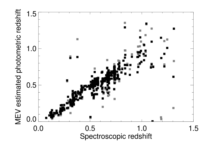
Figure 3: Minimum error variance (MEV) photometric redshift plotted against VVDS spectroscopic redshifts. Grey points represent those estimated with no magnitude prior, black points those estimated with the application of a magnitude prior. Limited to $R<23$.

For this set of brighter objects (60 per cent of the sample), redshift estimates are largely unchanged. Some outlier objects are have improved redshifts, but equally some are scattered further from the true value. The overall standard deviation of $z_{\mathrm{photo}}-z_{\mathrm{spec}}$ for each technique is not substantially changed, being $27$ per cent worse for the non-Bayesian case, but this is predominantly due to changes in outlier estimations.

As signal-to-noise decreases there is a substantial increase in the advantage gained by applying a prior, as the width of the $p(z)$ function decreases (Fig. 4). This is more substantial at high redshift since under the standard likelihood approach fainter objects (which dominate at high redshift) will produce a broader $\mathcal{L}(z)$, and it is in this region where the Bayesian approach provides the majority of the information. This effect is seen more clearly when data are binned by $R$ magnitude in Fig. 5 where we also see the actual $\delta z/(1+z)$ of MEV estimates. The relatively low $\delta z/(1+z)$ errors at the faintest magnitudes may be due to the high-confidence spectra from VVDS at such faint magnitudes being dominated by objects with particularly high-contrast spectral features suitable for making unusually good photometric redshift estimates, and should not necessarily be relied upon as being representative of the errors for faint objects in general.

For these MEV estimates we have removed redshift offsets of $0.028\times(1+z)$ and $0.023\times(1+z)$ for the non-Bayesian and Bayesian sets respectively. Such offsets are a result of the systematic effects described below and are dependent on various aspects of the photometry calibration. They can not be relied upon to be field independent and would in practice require some spectroscopic calibration to correctly remove.

In addition, we have eliminated outliers where $z/(1+z)$ has been misestimated by more than 3 standard deviations, calculated iteratively in unit magnitude bins from 18.5 to 24.5 (eliminating also two objects beyond 24.5). 51 outliers are eliminated in the non-Bayesian approach and 37 in the Bayesian approach. The error estimated from the width of the $p(z)$ distribution underestimates the true redshift error at high signal to noise, where the largest sources of errors are systematic effects such as relative calibrations of the passbands and variations in object spectra that are not represented in the templates. At lower signal to noise the range of possible colours covers the templates well enough that template incompleteness and passband uncertainties are less significant and allow for more accurate estimations of error based on the $p(z)$ width alone (see also Wolf et al. 2004 for a more detailed discussion of the properties of such estimation errors). In the case of the sample used here this transition to noise-dominated errors occurs at $R\lesssim 23$ and is the reason the $R<23$ cut was chosen in the examination of MEV estimates earlier.

Figure 4: Mean $\sigma_{z}/(1+z)$ (standard deviation of $p(z)$) in the case of no prior (upper line) and in the case of a magnitude prior (lower bold line). Results are binned in redshift intervals of 0.1 from z=0 to z=1.4 for objects where $R<24.5$

Figure 5: RMS redshift error as $\delta z/(1+z)$ as a function of R magnitude without prior (thin) and with (thick) along with width of probability functions scaled by $1/(1+z)$ (dashed lines), binned in 0.5 magnitude intervals from $R=18.5$ to $R=24.5$, $0<z<1.4$. Outliers, defined as objects more than 3s.d. (calculated iteratively) from the mean $\delta z/(1+z)$, are excluded (6 and 8 per cent for the Bayesian sample and non-Bayesian sample respectively).

Sensitivity and specificity for $UBVRI$ MEV estimates with and without a prior is given in Fig. 6 for the 400 objects with $R<23$. Outliers are included again, and we use a varying tolerance proportional to $1+z$ (as a fixed resolution $\delta\lambda/\lambda$ translates to fixed $\delta z/(1+z)$). Overall 73 per cent of objects have redshifts correct to $0.05\times(1+z)$ in the non-Bayesian case and 78 per cent in the Bayesian case. 92 per cent have redshifts correct to $0.1\times(1+z)$ in the non-Bayesian case, and 94 per cent in the Bayesian case, showing that single-valued estimates of redshifts are largely unchanged at brighter magnitudes. Error bars are estimates based on the assumption that objects fall in or out of the tolerance range according to the binomial distribution and are shown in order to give a better idea on the constraint of the true tolerance and can not indicate whether the techniques are significantly different. Performance by magnitude is also shown in Fig. 6 again showing broadly similar performances between the two methods for MEV estimates at brighter magnitudes, showing that gains are starting to be made as we approach the point at which these estimates will start to break down.

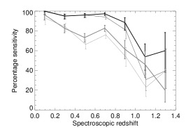
(a)

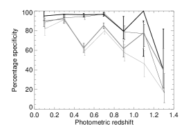
(b)

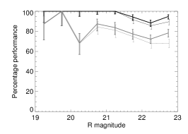
(c)

Figure 6: (a) Sensitivity, (b) specificity and (c) performance by magnitude of MEV photometric redshifts for $R<23$. Upper black lines show tolerance of $0.1\times(1+z)$ and lower grey lines show tolerance of $0.05\times(1+z)$. In each case the thin line represents results before a prior is applied and the thick line those afterwards. Error bars are estimates under the assumption that objects fall in or out of the tolerance according to the binomial distribution. In the case of performance by magnitude the concept of sensitivity and specificity do not apply as they are a result of binning by either photometric or spectroscopic redshift.

3.3.3 Using the full posterior probability distribution

At low signal-to-noise it becomes appropriate to avoid single-valued estimations (see Section 4). To compare sensitivity and specificity in the case where we aim to use summed normalised posterior distributions we define each as the percentage of the distribution within the given range, so sensitivity is defined as

$$\frac{\sum_{i}\int P_{i}(z)W_{i}(z)dz}{N_{i}}$$ (6)

where $i$ is the set of objects in a given bin of spectroscopic redshift, and specificity is defined as

$$\frac{\sum_{i}\int_{z_{A}}^{z_{B}}P_{i}(z)W_{i}(z)dz}{\sum_{i}\int_{z_{A}}^{z_{B}}P_{i}(z)dz}$$ (7)

where $i$ is the set of all objects, $z_{A}$ and $z_{B}$ denote the limits of the bin in consideration and we use a window function $W_{i}(z)$ as an additional constraint on the limits of the integrals so that

$$W_{i}(z) =1\text{ where }|z-z_{\mathrm{spec}_{i}}|<T(1+z_{\mathrm{spec}_{i}})$$

$$=0\text{ at all other points}$$

for a given tolerance $T$. With these definitions sensitivity and specificity are sums over equivalent regions in $z_{\mathrm{spec}}$ and $z$ to our earlier definitions.

Furthermore we define a performance binned by magnitude as

$$\frac{\sum_{i}\int P_{i}(z)W_{i}(z)dz}{N_{i}}$$ (8)

where $i$ is the set of objects in a given magnitude bin.

Sensitivity, specificity and performance plots in this case are given in Fig. 7. Sensitivity shows a small gain at almost all redshifts, and differences in specificity are also generally small. Overall performance is 49 per cent within a $0.05\times(1+z)$ tolerance without a prior and 53 per cent with, and 76 per cent within a $0.1\times(1+z)$ tolerance without a prior and 81 per cent with.

(a)

(b)

(c)

Figure 7: (a) Sensitivity, (b) specificity and (c) performance of photometric redshifts, full posterior definition, $R<24.5$. Upper solid lines show the percentage of the $L(z)$ or $p(z)$ function within a tolerance of $0.1\times(1+z)$ and lower dashed lines show tolerance of $0.05\times(1+z)$. In each case the thin line represents results before a prior is applied and the thick line those afterwards.

Fig. 8 show the 25th, 50th and 75th percentiles of summed $p(z)$ distributions in the cases without a prior and with a Bayesian prior over a range of spectroscopic redshifts and gives a clearer indication of regions where the prior has most effect. At low redshifts where objects tend to be brighter there is little difference but at higher redshifts and for fainter objects the estimates become much broader and generally occupy a range from about $z\approx 0.7$ upwards. The Bayesian estimates help resolve a bimodality with much lower redshifts around this region (which is the cause of the 25th percentile of the non-Bayesian distribution lying at such low redshift) and give a higher proportion of the estimation to the higher redshifts, although neither approach gives a particularly good match between the median distribution redshift and the spectroscopic redshifts.

Figure 8: Plots of the 25th, 50th and 75th percentile positions of summed posterior probabilities in redshift bins of 0.1 for $R<24.5$ in the case of no prior (thin lines) and a Bayesian prior (thick lines). Dashed lines indicate a line of $z_{\mathrm{photo}}=z_{\mathrm{spec}}$ and a region $\pm 0.1\times(1+z)$ tolerance.

As well as reproducing the distribution as accurately as possible, we must also examine whether selections from this distribution are unbiased representations of the true underlying redshifts. Clearly from examining Fig. 8 there is some degree of bias present. To check the severity of the bias, we also examine the mean photometric redshift in the two MEV cases and the mean of the summed posterior probabilities and the width of this distribution in the Bayesian case also in spectroscopic redshift bins of width 0.1 (Fig. 9). We perform a least-squares fit to determine a bias $b$ where $\langle 1+z_{\mathrm{photo}}\rangle=b(1+z_{\mathrm{spec}})$, weighting by the number of objects in each bin and inversely to the variance of MEV estimates or the width of the mean $p(z)$ estimate squared. Since the ability to make a reasonably unbiased estimate appears to break down above $z\approx 1$ as noise increases and the $z<0.1$ contains too few objects to rely upon we consider $0.1<z<1.0$ only. Non-Bayesian MEV estimates give a fit of $b=0.976\pm 0.003$, Bayesian MEV estimates give $b=0.977\pm 0.003$ and summed posterior probabilities give $b=0.978\pm 0.003$, indicating that there is no significant change in bias between the three approaches in that redshift range.

(a)

(b)

(c)

Figure 9: Mean estimated redshift for $R<24.5$ binned by spectroscopic redshift (a) without prior, (b) and (c) with prior. Error bars represent the $1\sigma$ spread in MEV estimates for (a) and (b) and the mean width of the summed $p(z)$ for (c). Lines indicate $z=z_{\mathrm{spec}}$ where there would be no bias.

As well as the bias in each bin, the spread in redshift estimates is also a concern. In Fig. 8 in the Bayesian case, half the probability distribution is contained within a region of $\delta z\approx 0.05$ at $0.1<z<0.2$ rising to $0.21$ at $0.9<z<1.0$. At higher redshifts the width is less stable, ranging from 0.28 to 0.45 at $z>1.0$. In comparison, the non-Bayesian case has $\delta z\approx 0.04$ at $0.1<z<0.2$ rising to $0.35$ at $0.9<z<1.0$, and from there as high as $1.03$ at higher redshifts.

A uniform distribution of redshifts in these bins would have half the distribution in $\delta z=0.05$, so there is a spread as would be expected due to the errors arising from estimating photometric redshifts, which presents a concern. In addition, there are significant outlier peaks in the probability distribution (some of which are picked up in Fig. 8 by the 25th percentile of the non-Bayesian distribution) which could disrupt an analysis, but the impact these regions have is reduced in the Bayesian approach, and this advantage is strongest for the faint galaxies where traditional methods break down.

Fig. 9 shows this also for MEV estimates, although the error bars here are influenced by the outlier regions mentioned above. In particular, the low redshift end shows larger error bars than might be expected from Fig. 8 as the second moment of the distribution is more sensitive to these outliers than the percentile positions. The MEV estimates also show less spread than the full posterior approach due to undersampling of the tails, and whilst this might appear initially a useful property we show in Section 4 that this can be highly problematic as signal-to-noise deteriorates. We return to this issue, and that of bias and higher order issues of the distribution in weak lensing analyses in Section 6.

3.4 Effects on redshift estimates from errors in the prior

There is a concern that the prior may not be the correct choice due to both measurement errors in the luminosity functions used in its calculation, and also due to systematic effects that might arise from the choice of fitted models to the luminosity functions and the treatment of the three types of galaxies used in the luminosity function calculation (such as the choice of spreading the luminosity function density evenly across the SED ranges).

A full analysis of the effect of measurement errors on the prior is computationally infeasible, and similarly attempting to make a full assessment of the impact of any effects of modelling choices and systematic effects arising from the method used to assign the luminosity function across SED types would be similarly infeasible. However, some assessment of the errors that would arise can be made by investigating a few special cases.

We have reanalysed the above sections with four further priors. Two of these have a faint end slope $\alpha$ of the red galaxies adjusted by $\pm 1\sigma$, and two have the $z=1.1$ value of $\phi^{\star}$ of the red galaxies adjusted by $\pm 1\sigma$. We adjust these parameters in preference to any others as the parameters most likely to make large changes to the prior.

High redshift values are chosen since adjustments to the low redshift parameters will have less effect, since most objects will be expected at higher redshift except for brighter objects which will already have well-constrained estimates and which will therefore be insensitive to the form of the prior.

Also, an overall shift in $\phi^{\star}$ affects the normalisation of the prior only, so we vary the value of this parameter for one class of galaxies rather than for all.

We ignore the variation in $M^{\star}$ typically has a lower impact on the resulting $\phi$ than the value of $\phi^{\star}$ does, and also since evolution of this parameter is halted at $z=1.0$ the models are more limited in the effect that variations in the $z=1.1$ point may have.

These four priors produce very little difference in the overall performance of the redshift estimates, with changes on the order of tenths of a percent corresponding to just a few objects falling in or out of the $0.05\times(1+z)$ and $0.1\times(1+z)$ tolerance bounds. For MEV estimates all priors have $78\%$ within $0.05\times(1+z)$ and $94\%$ within $0.1\times(1+z)$ for all but the prior with $\alpha$ raised, which performs marginally better at $95\%$ ($R<23$).With the full priors the figures are $53\%$ for all priors at $0.05\times(1+z)$ tolerances and $81\%$ for the original and $\alpha-1\sigma$ priors and marginally better with $82\%$ for the $\alpha+1\sigma$ and $\phi^{\star}(z=1.1)\pm 1\sigma$ priors ($R<24.5$).

This lack of significant difference can be partly ascribed to the fact that these are all brighter objects, and we examine this issue again in section 6 when we use simulations as deep as $R<25.5$ when this issue can be expected to have a greater impact. These results also of course only vary one parameter by $1\sigma$, and in reality some noise will apply to every parameter, but the small changes from varying these parameters which were chosen for maximum effect would not be expected to rise to problematic levels, and future constraints on luminosity function parameters can be incorporated to reduce the impact of the lack of knowledge we have of the form of the true underlying distribution of galaxies.

4 Photometric redshifts with high noise photometry

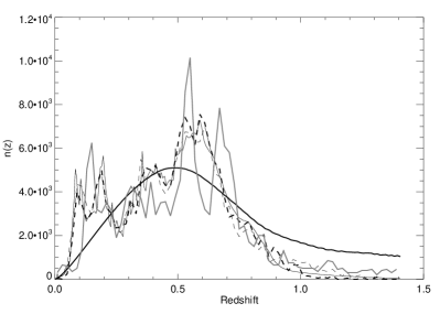
(a)

(b)

(c)

Figure 10: Estimated $n(z)$ distributions from a non-Bayesian MEV estimation (dashed line), Bayesian MEV (thick dashed line), summed posterior probability approach (thin continuous line) and a pure prior based solely on knowledge of the magnitude selection (thick continuous line). The distributions are for (a) $17<R<23$ (3,390 objects), (b) $23<R<24$ (5,285 objects) and (c) $24<R<25.5$ (18,885 objects). The fluctuations in the prior and summed posterior probability are slight artifacts from the process of calculating the prior distribution. For the $17<R<23$ set COMBO-17 MEV estimates are also included, shown as a solid grey line. 3 per cent of the sample do not receive a COMBO-17 estimate, and for the fainter samples this proportion rises considerably, so we do not show the distributions in these cases. All three sets of MEV estimates are binned in redshift intervals of $0.02$.

Perhaps the most significant benefit of a full posterior approach is in the case where redshift estimates traditionally break down owing to photometric noise and $L(z)$ becoming increasingly flat. In this situation one might conventionally set aside all objects with such poor photometry and in a weak lensing analysis simply estimate a single redshift distribution for all such objects. As faint objects are both more numerous and are generally at higher redshifts than more luminous ones the need to deal with them in an optimal manner is of greater concern than attempting to improve the already reasonably well-constrained redshifts of brighter objects.

The VVDS sample does not provide enough objects at a faint enough magnitude to study this effect so instead we consider a sample of 28,597 objects from the CDFS field of COMBO-17 with $17\leq R<25.5$ and is classed by COMBO-17 as a galaxy based on photometry (Wolf et al. 2004 describes this in more detail). Some objects have photometry that does not fit the templates sufficiently well and have extremely low likelihoods that produce a $p(z)$ distribution that due to computer rounding is zero at all redshifts, and these are excluded. There are not in general spectroscopic redshifts available for this sample, and for fainter objects reliable photometric redshifts are not available either (even when using all 17 bands). However, we can consider the distribution of photometric redshifts and compare them to expectations. Plots of the distributions of $UBVRI$-based MEV estimates along with the summed posterior probabilities and an expected distribution derived from the prior in three magnitude ranges are shown in Fig. 10, along with 17-band MEV estimates from COMBO-17 for the brightest set.

For brighter objects the estimates all converge on a result that includes more details of the large-scale structure in the field (Gilli et al. 2003, Le Fèvre et al. 2004 and Wolf et al. 2004 describe the CDFS as having rather pronounced large-scale structure). The peaks at $z\approx 0.15$ and $z\approx 0.6$ are both seen in the distribution of COMBO-17 photometric redshifts for example, although they are not so well resolved in the broad-band only estimations. The adjustments made by the prior are either small or, in the case of outlier correction, too rare to have a large effect on the overall distribution.

In the faint regime of $R>24$ the MEV estimates are clearly distorted by the inability to estimate a high redshift from a very broad $L(z)$ function (since $L(z)=0$ at $z>1.4$) and to a lesser extent the same effect at low redshift, and as a result the estimates cluster at the centre of the range of allowed estimates giving a distribution that is too sharply peaked. In the non-Bayesian case the relative coincidence of the peak of the distribution with that of the expected distribution is not due to any fundamental link between the two but that the expected distribution’s peak happens to fall near the centre of the estimation range. Even in the case of Bayesian MEV estimates the $p(z)$ distribution is still broad enough that the estimates cluster strongly in the central region of the estimation. These failures to make a good estimate of the distribution make MEV estimations unusable for faint objects. Maximum-likelihood (or maximum-posterior-probability) estimators would suffer a similar problem (although in the non-Bayesian case we would not expect the distribution to be so sharply peaked, it would still have little, if any, connection to the true distribution). Having a distribution that is affected by this issue, whether as extremely as demonstrated in Fig. 10 or to a lesser degree, would cause a bias in estimates of cosmological parameters from weak lensing measurements.

In contrast, the summed posterior distribution does not lose the contributions at the extremes and follows the expected distribution but with some modulation from any information that can be obtained from the photometry. Most importantly the severe bias in the distribution is eliminated and whilst there may be some present from the prior itself being generally biased compared to the true distribution, this could be reduced by constructing new priors as information on luminosity functions improves. We have therefore in the summed posterior probability approach moved smoothly from a well-constrained photometric redshift distribution towards a broadly estimated distribution providing a unified approach without having to decide upon a limiting accuracy of photometric redshifts beyond which we deal separately with any objects with poor photometry.

5 Sample priors

An alternative approach to dealing with this problem of bias is the “sample prior” described in Section 2.3 - a choice of prior that does accurately produce a set of estimates that reproduces $n(z)$ accurately, albeit at the cost of individual redshift estimates. This sample prior would have to be constructed through Monte Carlo simulations. By using the Bayesian prior to produce a sample set of simulated objects with a suitable overall distribution with colours and magnitudes based on the photometric redshift templates, and scattering these colours by an amount that might be expected from typical photometric errors we can construct a large simulation of a multicolour survey. These can be fed through a standard non-Bayesian redshift estimation algorithm which will scatter the original distribution to some estimated distribution and a suitable prior can be constructed that would convert the resulting estimated distribution back to the original.

This presents a practical problem in that the space to be sampled is very large, but since we expect $n$ to vary smoothly with both $z$ and $R$, and to a lesser extent SED we can still produce an attempt at a sample prior through fitting polynomial functions to the distributions to smooth over undersampled regions. An attempt at constructing a sample prior in this way succeeds in producing a distribution estimate approximately equivalent to a non-Bayesian approach but not as good as the summed posterior approach. Whilst this might be improved upon by constructing an improved prior the computational difficulty involved would outweigh the marginal gains that might be expected over the summed posterior estimation.

6 Effect on lensing calculations

To illustrate the effect of distortions in redshift distribution estimations on weak lensing studies we consider the predicted value of the critical surface mass density $\Sigma_{\mathrm{crit}}$ for lensing, which provides a scale by which the dimensionless mass surface density $\kappa$ can be converted to an estimated surface density. For a particular combination of lens and source redshifts, this critical density is given by

$$\Sigma_{\mathrm{crit}}=\frac{c^{2}}{4\pi GD_{d}}\beta$$ (9)

where

$$\beta=\langle D_{s}/D_{ds}\rangle$$ (10)

with $D_{d}$, $D_{ds}$ and $D_{s}$ being the angular diameter distances between observer and lens, lens and source and observer and source respectively.

The CDFS galaxy sample selected here has a distribution of redshifts, and hence for a given lens redshift, the value of $\Sigma_{\mathrm{crit}}$ is a weighted average over the distribution. At faint magnitudes the actual distribution is unknown, but we can illustrate the effect of the differences between the redshift estimators discussed above by calculating $\Sigma_{\mathrm{crit}}$ for each of the estimated distributions. We choose as test cases three lens redshifts ($z=0.3$, 0.5 and 0.7) and use the redshift distributions obtained from: (i) MEV estimates using a non-Bayesian approach; (ii) MEV with Bayesian prior; (iii) full posterior distributions; (iv) the prior distribution alone (based only on the magnitude limits with no colour information).

$17<R<25.5$

$z$	MEV	MEV	Full	Prior
	non-Bayesian	Bayesian	posterior	alone
0.3	9.96	11.87	10.78	9.56
0.5	4.02	5.04	4.96	4.67
0.7	2.01	2.48	2.71	3.05

$17<R<23$

$z$	MEV	MEV	Full	Prior
	non-Bayesian	Bayesian	posterior	alone
0.3	7.83	7.51	7.79	7.49
0.5	3.39	3.30	3.60	4.21
0.7	5.03	4.57	4.11	3.74

Table 3: Critical surface mass densities in two magnitude ranges for varying lens redshifts and distribution estimates, $10^{8}M_{\odot}h\mathrm{kpc}^{-2}$

For the CDFS sample with $17<R<25.5$ we find values of critical density shown in Table 3. At low lens redshifts the differences between the densities are not dramatic (as is expected as $\beta$ changes most near the lens where the estimates all largely agree), but at higher lens redshifts the differences can be larger, most notably between the non-Bayesian estimates and the three other estimates at a lens redshift of $0.7$, where the non-Bayesian estimate differs from the others by between $20\%$ and $50\%$. In addition, although the Bayesian MEV estimates look generally reasonable, the fact that a large number of objects that other estimates place in front of the lens are classified instead as background objects could lead to these “misclassified” objects diluting the shear signal and causing the lens mass to be underestimated, despite getting an apparently reasonable estimate of $\Sigma_{\mathrm{crit}}$ in the above calculation (such effects are investigated below with a Monte-Carlo simulation).

The majority of the disagreement in the above test arises from the $R>23$ objects, as can be seen when the critical densities for brighter objects alone ($17<R<23$) are considered. In this case, where the colours of the objects are the primary source of information rather than the prior, the first three distributions all provide very similar results, but the prior alone generally disagrees slightly. The exception is the $z=0.7$ lens, where the background sources are all in the tail of the redshift distribution and are close to the lens, so that slight changes in the estimation of $n(z)$ have a dramatic effect owing to the steep variation in $\beta$ near the lens redshift.

We can use a Monte-Carlo simulation to test the effects of poor redshift estimation and the resulting change in mass estimates owing to errors in individual values of $\beta$ and to foreground/background errors. We produce a Monte Carlo simulation of COMBO-17 5-band data in which 10,000 objects are drawn randomly from the template set and assigned an $R$-band magnitude according to the prior distribution. Each object has its $UBVRI$ fluxes calculated from the template colours and the assigned $R$-band magnitude, and each of the five fluxes is scattered assuming a Gaussian error typical for a background-limited signal in COMBO-17.

After estimating redshifts for this simulated dataset, we have a set of simulated objects with a ‘true’ redshift $z_{i}$ for even the faintest objects, along with an estimated photometric redshift $z_{\mathrm{est}_{i}}$. We then assign each object a convergence

$$\kappa_{i}=\frac{\Sigma}{\Sigma_{\mathrm{crit}}(z_{i})}$$ (11)

for a fixed surface mass density $\Sigma$, and where foreground objects are given a convergence of zero.

Next, we calculate an estimate of the surface mass density that would be inferred from its convergence and estimated redshift value,

$$\Sigma_{i}=\Sigma_{\mathrm{crit}}(z_{\mathrm{est}_{i}})\kappa_{i}$$ (12)

$D_{s_{\mathrm{est}_{i}}}>D_{d}$, and with a final overall estimate of the surface mass density $\hat{\Sigma}$ being determined as

$$\hat{\Sigma}=\langle\Sigma_{i}w_{i}\rangle/\langle w_{i}\rangle.$$ (13)

The weighting $w_{i}$ is a foreground/background parameter and is 1 in the case of MEV estimates where $D_{s}>D_{d}$ and 0 elsewhere, and in the case of a posterior distribution or a prior is given by

$$w_{i}=\int_{z_{d}}^{z_{\mathrm{max}}}p(z)dz.$$ (14)

Resulting mass estimates in each case are given in Table 4 for lenses at $z=0.3$, 0.5, 0.7 and 0.9. The prior alone performs much better in this case as the ‘true’ redshift distribution is drawn directly from it. The unusually good result for the non-Bayesian MEV estimates at $z=0.5$ may be due to various effects of misestimations cancelling out by chance. The dramatically poor result for the $z=0.9$ lens for these estimates suggest that this choice would be a poor one in general. Even the Bayesian MEV estimates show significant misestimations of the surface mass density and can’t therefore be recommended as an approach unless the problematic fainter objects are excluded (at $R<23$ the Bayesian MEV estimated densities are all within $2\%$ of the true value except for a lens redshift of $0.9$, whereas the non-Bayesian MEV estimated densities deviate by more than $2\%$ for all the lens redshifts).

$z$	MEV	MEV	Full	Prior
	non-Bayesian	Bayesian	posterior	alone
0.3	1.05	1.02	1.03	1.01
0.5	1.01	1.12	1.01	0.99
0.7	1.17	1.22	1.03	0.99
0.9	1.61	1.23	1.01	1.04

Table 4: Surface mass densities (ratio to true value) for four distribution estimates and four lens redshifts from simulated data, $17<R<25.5$.

When the reconstructed mass densities are dramatically incorrect they overestimate. This is understandable if the numbers at the highest redshift are underestimated, as is seen in the MEV estimations at low signal-to-noise in Fig. 10. Galaxies in this region have their redshifts underestimated, and as a result the calculated lensing mass must be higher to produce the same lensing effect at a lower distance from the lens.

For the faintest galaxies in a real survey however, the shape measurements will also be noisy, and will be downweighted, which will generally reduce the effect of photometric redshift errors. This reduction in the likely errors compared to the Monte Carlo simulations given here will not be of as much benefit for those lensing systems at high redshift, since the background sources in this case will all tend to be fainter and have largely comparable weightings.

We return briefly to the issue raised in Section 3.4, where the effect of noise on the measurements of the GLFs was considered. Using the same priors as used in that section ($\alpha$ varied by $\pm 1\sigma$ and $\phi^{\star}(z=1.1)$ for red galaxies varied by $\pm 1\sigma$) we recalculate the surface mass densities of Table 4. The results are given in Table 5. The differences are still small (a few tenths of a percent difference in surface mass densities between the various priors) and whilst the error on the prior may be larger and the inaccuracy in the prior may be large enough to have appreciable effects, they are still likely to be much smaller than those effects that arise from a non-Bayesian or MEV estimation approach.

$z$	Unaltered	$\alpha+1\sigma$	$\alpha-1\sigma$	$\phi^{\star}+1\sigma$	$\phi^{\star}-1\sigma$
0.3	1.028	1.029	1.028	1.029	1.029
0.5	1.014	1.015	1.014	1.015	1.014
0.7	1.026	1.030	1.028	1.031	1.027
0.9	1.008	1.009	1.011	1.011	1.009

Table 5: Surface mass densities (ratio to true value) for full posterior distribution estimates and four lens redshifts from simulated data, $17<R<25.5$, using priors calculated from altered GLF parameters.

We also return to the issue of biases in redshift estimates and issues of higher order moments of the posterior probability distribution. Section 3.3.3 gave estimates of the bias of photometric redshifts, expressed as $\langle 1+z_{\mathrm{photo}}\rangle=b(1+z_{\mathrm{spec}})$. Fitting to the VVDS sample at $0.1<z<1.0$ gave $b=0.978$, which would lead to estimated redshifts generally falling slightly below the true redshift, and therefore lead to a slight overestimation in lensing masses. In the case of a single source at $z=1$, for lens redshifts of 0.3, 0.5 and 0.7 the misestimations are $1.2\%$, $2.8\%$ and $6.7\%$ respectively, much lower than those arising from choosing an alternative estimation technique (although this bias was measured only for the restricted range of objects described earlier, and will be more of a problem at $z>1$).

Higher order moments of the posterior probability are also a concern, since the critical densities we estimate are based on $\beta=\langle D_{s}/D_{ds}\rangle$, and $\langle\beta\rangle$ is not proportional to $\langle z\rangle$.

However, since $\beta$ approaches a constant as $D_{s}$ increases, variations in the distribution at high redshift do not impact the estimated lensing mass as much as estimates at low redshift. As a result, for low lens redshifts the shape and width of the distributions are not a major concern, since close to the lens where $\beta$ is varying most rapidly the sources are also at low redshift and, being generally brighter, have tightly constrained distributions. At high lens redshifts the distribution widths and shapes are much more of a concern as they will be broader and cover regions of significant variation in $\beta$. In these cases estimates of the bias alone may prove insufficient and the best approach to estimating resulting errors would likely be further simulations.

The conclusion from these tests is that the full posterior approach is capable of providing lensing estimates that agree with previously used photometric techniques in the $R<23$ regime, and yet also agrees for fainter samples with the modelled redshift distributions, providing consistent estimated lens masses over a broad range of lens redshifts. In these tests Bayesian MEV estimates perform better than pure likelihood estimates, but are likely to be less good in 3-D lensing analyses. In such analyses, the distribution of mass is estimated as a function of redshift using the photometric redshifts of the observed galaxies. Hence we expect the estimated mass distribution will be even more sensitive to any systematic poor estimation of redshifts than the tests that we have described above.

7 Conclusions

Extraction of the full information content of future generations of weak lensing surveys will require extensive use of photometric redshifts, applied to both 2D and 3D analyses. Weak lensing signals are concentrated towards the magnitude limits of surveys, and yet it is here that photometric measurement errors make photometric redshift estimation the most unreliable. These errors lead not only to a broad distribution of redshift uncertainty, but also to increasing severity of the degeneracy between galaxy type and redshift that frequently leads to multiple solutions for an estimated redshift. Furthermore, the effect of measurement errors is to make the sample distribution of estimated redshifts different from the true distribution of redshifts, which inevitably leads to bias in the values of cosmological parameters estimated from the overall sample.

In this paper we have considered the Bayesian solution to this problem, and have shown that using the full Bayesian posterior probability distribution for estimated redshifts allows such biases to be eliminated, provided a prior distribution, here based on knowledge of the galaxy luminosity function and its evolution, is known. Using photometric and redshift data from the COMBO-17 sample, we have compared the full Bayesian approach with pure likelihood estimation and minimum error variance (MEV) methods and show that, although there is little to choose between methods at bright magnitudes, the full Bayesian method is significantly less biased at faint magnitudes. Furthermore, the Bayesian method allows the sample distribution of estimated redshifts to tend smoothly towards the prior distribution at the faintest limits of a survey.

Applying the method to simulated weak lensing signals, we show that reconstruction of lensing mass density in the presence of photometric redshift errors can lead to biases in excess of 20 percent in 2D lensing analyses unless the Bayesian method is adopted. We anticipate that 3D lensing analyses will be even more susceptible to this effect, but we postpone to a future paper a full incorporation of the Bayesian probability approach into 3D lensing analysis.

ACKNOWLEDGEMENTS
EME acknowledges the support of a PPARC Graduate Studentship. CW acknowledges the support of a PPARC Advanced Fellowship. We also thank David Bacon and Devinder Sivia for many helpful comments.

References

- Bacon & Taylor (2003) Bacon D.J., Taylor A.N., 2003, MNRAS, 344, 1307
- Baum (1962) Baum W.A., 1962, in IAU Symposium No. 15, p390
- Bolzonella, Miralles & Pelló (2000) Bolzonella M., Miralles J.-M., Pelló R., 2000, A&A, 363, 476-492
- Brown et al. (2003) Brown M.L., Taylor A.N., Bacon D.J., Gray M.E., Dye S., Meisenheimer K., Wolf C., 2003, MNRAS, 341, 100
- Benítez (2000) Benítez N., 2000, ApJ, 536, 571-583
- Brodwin et al. (2003) Brodwin M., Lilly S.J., Porciani C., McCracken H.J., Le Fevre O., Foucaud S., Crampton D., Mellier Y., 2003, ApJ. submitted, preprint (astro-ph/0310038)
- Csabai et al. (2003) Csabai I. et al., 2003, AJ, 125, 580
- Cohen (2002) Cohen J.G., 2002, ApJ, 567, 672-701
- Collister & Lahav (2004) Collister A.A. & Lahav O., 2004, PASP, 116, 345-351
- Connolly, Csabai & Szalay (1995) Connolly A.J., Csabai I., Szalay A.S., 1995, AJ, 110, 2655-2664
- Faber et al. (2005) Faber S.M. et al., 2005, ApJ submitted, preprint (astro-ph/0506044)
- Le Fèvre et al. (2004) Le Fèvre O. et al., 2004, A&A, 417, 839-846
- Fioc & Rocca-Volmerange (1997) Fioc M., Rocca-Volmerange B., 1997, A&A, 326, 950
- Gilli et al. (2003) Gilli R. et al., 2003, ApJ, 592, 721-727
- Heavens (2003) Heavens A., 2003, MNRAS, 343, 1327
- Heymans & Heavens (2002) Heymans C., Heavens A., 2003, MNRAS, 339, 711
- Hsieh et al. (2005) Hsieh B.C., Yee H.K.C., Lin H., Gladders M.D., 2005, ApJS, 158, 161
- Hu (1999) Hu W., 1999, ApJ, 522, 21
- Ilbert et al. (2004) Ilbert O. et al., 2004, A&A submitted, preprint (astro-ph/0409134)
- King & Schneider (2003) King L., Schneider P., 2003, A&A, 398, 23-30
- Pickles (1998) Pickles A.J., 1998, PASP, 110, 863
- Taylor (2002) Taylor A.N., 2002, Phys. Rev. Lett. submitted, preprint (astro-ph/0111605)
- Taylor et al. (2004) Taylor A.N. et al., 2004, MNRAS, 353, 1176
- vanden Berk et al. (2001) Vanden Berk D.E. et al., 2001, AJ, 122, 549
- Wadadekar (2005) Wadadekar Y., 2005, PASP, 827, 79-85.
- Wolf et al. (2001) Wolf C., Meisenheimer K., Röser H.-J., 2001, A&A, 365, 660-680
- Wolf et al. (2003) Wolf C., Meisenheimer K., Rix H.-W, Borch A., Dye S., Kleinheinrich M., 2003, A&A, 401, 73-98
- Wolf et al. (2004) Wolf C. et al., 2004, A&A, 421, 913-936