[astro-ph/0607299] 1 INTRODUCTION

Photometry of the Magnetic White Dwarf
SDSS 121209.31+013627.7

C. Koen¹ and P.F.L. Maxted²
1 Department of Statistics, University of the Western Cape, Private Bag X17, Bellville, 7535 Cape, South Africa
2 Astrophysics Group, Keele University, Keele, Staffordshire ST5 5BG, United Kingdom

ABSTRACT. The results of 27 hours of time series photometry of SDSS 121209.31+013627.7 are presented. The binary period established from spectroscopy is confirmed and refined to 0.061412 d (88.43 minutes). The photometric variations are dominated by a brightening of about 16 mmag, lasting a little less than half a binary cycle. The amplitude is approximately the same in $V$ , $R$ and white light. A secondary small brightness increase during each cycle may also be present. We speculate that SDSS 121209.31+013627.7 may be a polar in a low state.

Key words: stars: low mass, brown dwarfs - stars: individual: SDSS 121209.31+013627.7 - stars: variables: other - binaries: close

1 INTRODUCTION

The white dwarf star SDSS 121209.31+013627.7 (abbreviated “SDSS 1212+0136” below) has a mean surface magnetic field $\sim 7$ MG, derived from Zeeman splitting of its Hydrogen absorption lines (Schmidt et al. 2005a). Spectra also show weak H $\alpha$ emission, implying a composite system. Despite the relatively low temperature of the white dwarf ( $\sim 10000$ K) there are no overt signs of the presence of the companion in photometry blueward of the $J$ band. This suggests that the companion is very cool – probably a brown dwarf (Schmidt et al. 2005a). Radial velocity changes and modulation of the H $\alpha$ equivalent width allow a binary period of about 90 minutes to be deduced. The orbital inclination appears to be high.

Given the close proximity of the two components (implied by the short binary period), the cool companion is strongly irradiated by the white dwarf. The H $\alpha$ emission may then be ascribed to re-radiation from the facing hemisphere of the cool object.

Since radiation from the white dwarf is dominant even at $J$ , Schmidt et al. (2005a) suggested follow-up photometry and spectroscopy further into the infrared, at $K$ . The authors also speculated that optical photometry may be useful to test for pulsation in the white dwarf, and to search for possible eclipses of the white dwarf by the unseen companion. The latter two aims motivated the observations reported here.

The experimental work is described in section 2, and the analysis of the data in section 3. Section 4 deals with the modelling of the photometry, and conclusions are presented in section 5.

2 THE OBSERVATIONS

All measurements were made with the SAAO (South African Astronomical Observatory) CCD camera mounted on the SAAO 1.9-m telescope at Sutherland, South Africa. The camera, which has a field of view of about 2.5 arcmin $\times$ 2.5 arcmin, was operated in $2\times 2$ prebinning mode, which gave a reasonable readout time of 20 seconds. A log of the observations is given in Table 1. Measurements comprising the last three runs were made in white light, i.e. no filter was placed in the light beam; this allowed shorter exposure times to be used, and hence better time resolution to be obtained. The effective wavelength of these white-light observations is between $B$ and $V$ , but with a very wide bandpass. Photometric reductions were performed using an automated version of DOPHOT (Schechter, Mateo & Saha 1993).

Typically only four measurable stars were visible in the field of view. The brightest two stars were used to differentially correct the photometry for atmospheric effects. The remaining two stars were of comparable brightness, and the non-programme star is therefore a useful “check” star for the photometry of SDSS 1212+0136. The nightly mean differences [in the sense (check star)-(programme star)] are shown in Table 1. There is some evidence for changes in the mean light level of SDSS 1212+0136 from night to night. The last column of the Table gives the standard deviations of the photometry of the check star: since its mean magnitude is quite similar to that of the programme star, these values probably constitute reasonable estimates of the photometric accuracies of the measurements of SDSS 1212+0136. Standard deviations for the two local comparison star measurements were typically half (filter-less observations) or one third ( $V$ -band) of those in the Table.

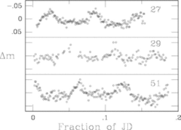
The results of the three white-light runs are plotted in Fig. 1. The data have been adjusted to have the same nightly mean values. Bumps in the light curves, roughly 0.05 d apart, are clearly visible. It is noteworthy that the scatter in the three lightcurves is not correlated with the quality of the nights, as measured by the $\sigma$ -values in Table 1, but rather with the mean light level of the observations ( $\Delta z$ -column in Table 1). The correlation is in the sense that the brighter SDSS 1212+0136, the more noisy its white light lightcurve.

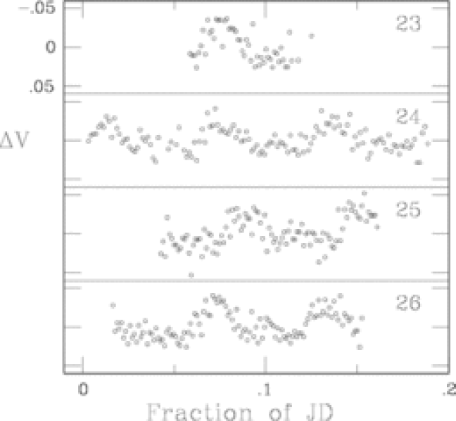
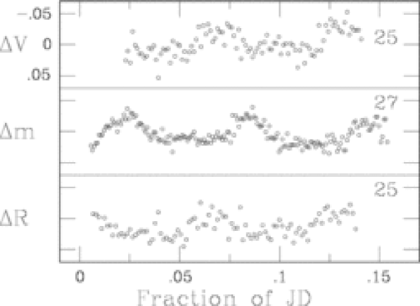
The $V$ -band lightcurves (Fig. 2) are generally more noisy than those obtained without any filter: this is probably mainly due to the fact that the brightness in $V$ is substantially ( $\sim 1.5$ mag) fainter than in white light. The reader’s attention is drawn to the small brightness increases about midway between the bumps in the light curves: see particularly the lightcurves for HJD 2453824 and 2452826. Fig. 3 compares results in $R$ , $V$ and white light: it is interesting that the sizes of the bumps in the light curves are comparable despite being observed through different filters.

3 DATA ANALYSIS

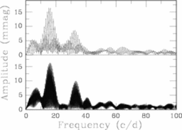
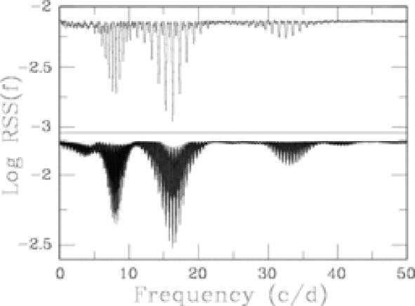
Fig. 4 shows the amplitude spectra of all the $V$ data (top panel) and all the data acquired without any filter (bottom panel). (In order to avoid confusion we mention that the term “amplitude” should be understood to mean “semi-amplitude”; we will refer explicitly to “peak-to-peak amplitude” when that meaning is intended). A telling feature of the two spectra is excesses of power around frequencies 8, 16 and 32 d^-1. Schmidt et al. (2005a) determined a period of 0.065 d (frequency $f=15.4$ d^-1) for the star: this evidently corresponds to the main peak at about 16 d^-1, with the other two frequencies being respectively the first harmonic and a sub-harmonic. The sub-harmonics are evidently induced by cycle-to-cycle variations in the observed lightcurves, and will be ignored in what follows: the statistical model

	$\displaystyle m(t)$	$\displaystyle=$	$\displaystyle\sum_{j=1}^{2}C_{j}\cos(2\pi jft+\phi_{j})+e_{t}$		(1)
		$\displaystyle=$	$\displaystyle\sum_{j=1}^{2}[A_{j}\cos(2\pi jft)+B_{j}\sin(2\pi jft)]+e_{t}$		(1)

is fitted to the data $m(t)$ . In (1); $C_{1}$ , $C_{2}$ and $\phi_{1}$ , $\phi_{2}$ are the amplitudes and phases associated with the fundamental frequency $f$ and its first harmonic $2f$ ; and $e_{t}$ is an error term. Expansion of the cosine form into the sum of a cosine and a sine [the second form in (1)] leaves the frequency $f$ as the only nonlinear parameter in a regression of the observations $m_{t}$ on time $t$ .

The results of fitting the model (1) to the $V$ -data and filter-less observations can be seen in Fig. 5, for a range of trial frequencies $f$ . Note that for a given value of $f$ , the parameters $\mu$ , $A_{1}$ , $A_{2}$ $B_{1}$ and $B_{2}$ all follow from minimisation of the sum of squares

SS(f)=\sum_{t}\left\{m(t)-\sum_{j=1}^{2}[A_{j}\cos(2\pi jft)+B_{j}\sin(2\pi jft)]\right\}^{2}\;.

(2)

The logarithm of the minimised $SS(f)$ , denoted $RSS(f)$ (“residual sum of squares”) is plotted in the figure.

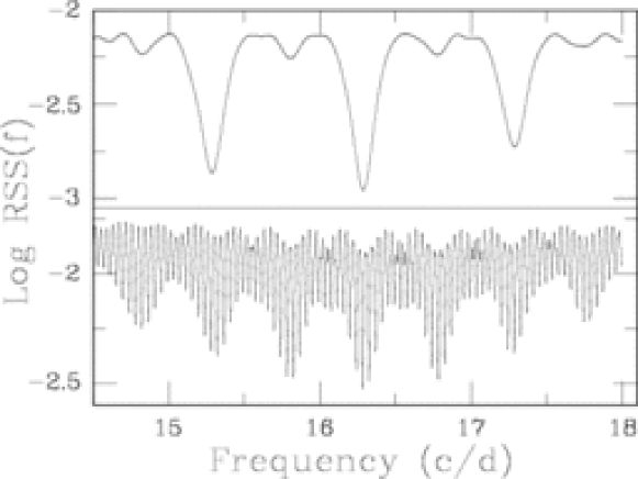
Fig. 6, which is a more detailed view of the frequency interval of principal interest, shows very good agreement between the $V$ and white light results. Of course, the frequency resolution in the latter is considerably better, since the observations cover a longer time baseline (24 versus 3 days). It is particularly useful that the alias peaks near 15.8 and 17.8 d^-1 in the bottom panel of the diagram can be discounted since there are no substantial counterparts in the top panel.

The best-fitting frequencies $f_{*}$ are 16.288 d^-1 ( $V$ data) and 16.2836 d^-1 (white light). The interpretation of Fig. 6 is aided by noting that the quantity

\Lambda=(N-p)\left[\frac{\sum_{t}RSS(f)}{\sum_{t}RSS(f_{*})}-1\right],

(3)

which is the approximate Gaussian likelihood ratio, has an approximate $\chi^{2}_{1}$ distribution (i.e. chi-squared with one degree of freedom – see Gallant 1987 for the theory, and Koen 2004 for an application very similar to the present one). In (3), $N$ is the number of observations, and $p$ is the number of estimated parameters. In Eqn. (2), the parameters $A_{1}$ , $A_{2}$ , $B_{1}$ , $B_{2}$ and $f$ are estimated; in addition, the nightly offsets from a common mean value were calculated. It follows that $p=9$ for the $V$ data, $p=8$ for the white light observations.

Koen (2004) showed that for large $N$ (a few hundred or more), (3) implies that $\alpha$ -level confidence intervals for $f$ are given by

\Delta\log RSS=\log RSS(f)-\log RSS(f_{*})\stackrel{{\scriptstyle<}}{{~{}}}\frac{\chi^{2}_{1}(\alpha)}{N-p}\;.

(4)

In the present case the number of observations is 394 ( $V$ ) or 526 (white light), hence $\Delta\log RSS\approx 0.0100,0.0074$ respectively, for 95% confidence intervals [ $\chi^{2}_{1}(0.95)=3.84$ ]. The implication is that the aliases are comfortably outside the 95% confidence interval for the best frequency.

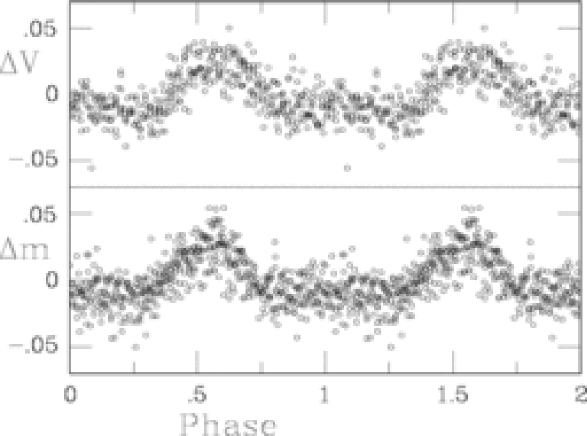
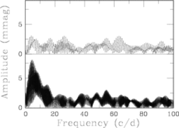
Details of the best fitting solutions for the two datasets appear in Table 2. Also shown are the results of fitting the model in (1) to the $R$ -band data using $f=16.2836$ d^-1. Fig. 7 shows the data folded with respect to the best-fitting period, and amplitude spectra of the residuals are plotted in Fig. 8. It is interesting that the model has accounted for most of the $V$ -band power at the sub-harmonic, but little of the power in the sub-harmonic of white light observations. We ascribe this to greater variability in the shape and/or mean level of the filter-less measurements.

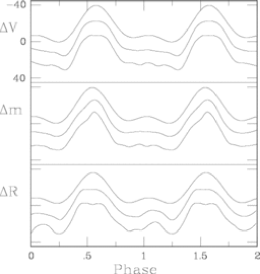
Since the folded lightcurves are noisy their shapes are extracted by statistical means. First, the fits of Eqn. (1) provide the top curves in each of the three panels in Fig. 9. The small bumps near phase 0.5 referred to at the end of section 2 clearly form part of that simple parametric model. The remaining two curves in each panel were obtained by a non-parametric smoothing method known as “loess” (Cleveland & Devlin 1988; Cleveland, Devlin & Grosse 1988). The technique is akin to a weighted moving average, but can be applied to irregularly spaced data. In our implementation, we used local quadratic fits to the phased data in Fig. 7, and to the similarly phased $R$ -band data. Window widths of 0.4 (middle curves) and 0.3 (bottom curves) of a cycle were used for the abundant $V$ and white-light data; for the sparser $R$ data the window widths were 0.5 and 0.4 of a cycle.

The smaller the window width used the more detail emerges, at the risk of extracting spurious feature due to noise in the data. The following generalities nonetheless seem plausible:

(1)

The lesser bump in the light curve seems to be a real feature, and may increase in amplitude towards longer wavelengths.
(2)

Small bumps aside, there appears to be a systematic decrease in brightness between the end of one large bump and the onset of the next.
(3)

There is an impression that the large bumps may be flat-topped in $V$ and $R$ , but not in white light.
(4)

The large bumps appear symmetrical in $V$ and $R$ , but not in white light.

The next section of the paper deals with attempts to explain the light curve shapes.

4 PHYSICAL MODELS

We assume that the main periodicity in our lightcurves is the same as the orbital period of SDSS 1212+0136, given that it is very similar to the period seen in the radial velocity of the weak H $\alpha$ emission line by Schmidt et al (2005a). We used the four radial velocities presented in their fig. 3 for the dates listed in their fig. 2 to re-calculate the semi-amplitude of the orbit, $K$ , using a least-squares fit of a cosine with the data equally weighted and with the orbital period fixed at the value derived above. Other free parameters in the fit were the time of maximum positive radial velocity, $T_{0}$ and the systemic velocity, $\gamma$ . We account for the finite exposure time of about 500s in our fitting procedure and find that this increases the value of $K$ by about 8 km s^-1. We find $K=355\pm 6$ km s^-1, $\gamma=33\pm 4$ km s^-1 and $T_{0}=0.2801\pm 0.0003$ days, where $T_{0}=0$ corresponds to 0000UT 2005 May 14. With this value of $K$ we find that the companion is close to filling its Roche lobe. For example, for a companion with a mass of $0.05~{}M_{\odot}$ the radius of the Roche lobe is 0.11 $R_{\odot}$ , which is comparable to the radius expected for a typical brown dwarf (Baraffe et al. 2003).

It is reasonable to assume that the variability in the lightcurves is the reflection effect caused by the irradiation of one side of the companion by the white dwarf. We can estimate the amplitude of the reflection effect in magnitudes, $\Delta m_{\rm ref}$ , using

\Delta m_{\rm ref}\approx-2.5\log\left(\frac{f_{\rm opt,wd}+f_{\rm int}f_{\rm opt,ref}}{f_{\rm opt,wd}}\right),

where $f_{\rm int}\approx 0.01$ is the fraction of the white dwarf’s light intercepted by the companion, $f_{\rm opt,wd}$ is the fraction of the white dwarf’s light emitted at wavelengths covered by our white light, V-band and R-band photometry and $f_{\rm opt,ref}$ is the fraction of the intercepted flux re-emitted over the same wavelength region. We used the pure hydrogen model atmosphere spectra for a 10,000 K white dwarf by Rohrmann (2001) to estimate $f_{\rm opt,wd}\approx 0.36$ . If the irradiated hemisphere of the companion re-emits all the intercepted flux and we assume an effective temperature for the companion of about 1600 K, then the net flux from this irradiated hemisphere is equivalent to an effective temperature of 1900 K. For blackbody radiation, this gives $f_{\rm opt,ref}<0.01$ , which would imply that the reflection effect would be undetectable at optical wavelengths. More realistically, the re-emitted spectrum is likely to be dominated by radiation from the point on the companion closest to the white dwarf, which will be hotter than the average temperature on the irradiated hemisphere. Even so, the maximum value of $f_{\rm opt,ref}$ for blackbody radiation, which occurs for temperatures of about 8500 K, is $f_{\rm opt,ref}\approx 0.45$ . For this extreme value we obtain a peak-to-peak amplitude $\Delta m_{\rm ref}=0.014$ , less than half the observed amplitude. We conclude that the main cause of the photometric variability in SDSS 1212+0136 is not the reflection effect, but that the reflection effect may be a small contribution to the variability, .e.g., it may be the cause of the small bump seen in the lightcurve.

Similar arguments can be applied to the H $\alpha$ emission line, as has been done by Schmidt et al. (1995) for the white dwarf – M-dwarf binary star GD 245. In the case of this emission line we use the flux of ionizing photons incident on the brown dwarf surface to calculate an upper limit to the apparent flux in the H $\alpha$ emission line by assuming that one H $\alpha$ photon is emitted for every incident photon below the Lyman limit and that there are no other sources of H $\alpha$ emission. The equivalent width of the H $\alpha$ line is then given by

{\rm EW}(\rm H\alpha)\approx f_{\rm int}\cdot Q=f_{\rm int}\frac{\int_{0}^{912{\rm\AA}}S_{\lambda}d\lambda}{S_{\lambda}(H\alpha)},

where $S_{\lambda}$ is the photon flux from the white dwarf. This can be compared directly to the value of EW(H $\alpha$ ) $\approx 10$ Å presented by Schmidt et al (1995). We used the pure hydrogen model atmosphere of Rohrmann (2001) for $T_{\rm eff}=$ 10,000 K, $\log g=8$ to find $Q=0.33$ . For this value of $Q$ the equivalent width of the H $\alpha$ is expected to be $<0.01$ Å.

Given the large observed amplitude and the strength of the H $\alpha$ emission line, it appears that there is an additional source of radiation in the system. Accretion onto the white dwarf is a likely candidate. We can estimate the accretion rate by assuming that all of the energy due to accretion intercepted by the companion is emitted in the H $\alpha$ line. Using the distance of 145 pc estimated by Schmidt et al. (2005a), we find the accretion rate onto the white dwarf is about $10^{-13}M_{\odot}/y$ . This is in good agreement with the mass transfer rates onto white dwarfs from the solar-type wind of the low mass companion in other pre-polar binary systems (Schmidt et al. 2005b). Assuming that there is accretion onto the magnetic white dwarf in this binary, it is likely that cyclotron emission contributes to the optical variability we have observed. We do not consider it worthwhile to discuss a model for cyclotron emission in detail here given the large number of parameters required for such a model and the small number of constraints that can be imposed on these parameters given the existing observations.

If there is an accretion hot spot on the white dwarf where material from the companion is channelled onto one of its magnetic poles, then the change in brightness could be due to the change in visibility of the spot as the white dwarf rotates. Occultation as the spot disappears over the limb of the white dwarf, or non-isotropic emission from the spot, could explain the variability. A very approximate estimate of the characteristic temperature of such a hot spot can be made by assuming that the increase of about 5 percent in brightness at the maximum of the lightcurve is due to optically thick radiation from a spot with a radius of 5 – 10 percent of the white dwarf radius powered by accretion at a rate equivalent to 5 percent of the luminosity of the white dwarf. In this case the temperature is 15 000 – 20 000 K. These high temperatures are consistent with the observation that the increase in brightness is similar in the $V$ and $R$ bands, and the white-light photometry.

5 CONCLUSIONS

We confirm and refine the orbital period of about 90 minutes for SDSS 1212+0136 seen by Schmidt et al. (2005a) using lightcurves in various optical bands. There are no obvious eclipses in our lightcurves of SDSS 1212+0136, neither is there any sign of pulsation.

The lightcurves all show a brightness enhancement at optical wavelengths of about 5 percent lasting about 0.4 of an orbital cycle. The effect shows little change in amplitude with colour. The amplitude of the effect, the strength of the H $\alpha$ emission line and the variability of the photometry of SDSS 1212+0136 all point to ongoing accretion in this binary at a rate of at least $10^{-13}M_{\odot}/y$ . The companion to the white dwarf is close to filling its Roche lobe, which suggests that SDSS 1212+0136 may be a normal polar in a low state. However, there are no recorded high-states for this star. The five epochs of photographic photometry in the USNO B-1 catalog all show SDSS 1212+0136 at about 18th magnitude (Monet et al. 2003). Schmidt et al. (2005a) have also discussed the possibility that SDSS 1212+0136 is a polar in a low state but conclude that it is unlikely. A better estimate of the mass transfer rate can be made using observations at X-ray wavelengths, since the X-ray flux will be due entirely to accretion.

There is reasonable evidence for a smaller brightness increase during the orbital cycle, approximately midway between large brightness enhancements. Given its orbital phasing, amplitude, and possible increase with increasing wavelength, we speculate that these smaller lightcurve bumps may be due to a reflection off the companion.

A better estimate of the mass of the companion will require a radial velocity curve for the white dwarf. This will be difficult if the Balmer lines are variable in profile since the semi-amplitude of the white dwarf’s spectroscopic orbit is expected to be only K ${}_{\rm WD}\approx 55$ km/s.

ACKNOWLEDGMENTS

Exchange of ideas with Dr. Dave Kilkenny (SAAO) was helpful. PM thanks Dr Coel Hellier and Dr Boris Gänsicke for discussing their opinions of the lightcurves. Telescope time allocation by SAAO is gratefully acknowledged.

REFERENCES

Baraffe I., Chabrier G., Barman T. S., Allard F., Hauschildt P. H., 2003, A&A, 402, 701

Cleveland W.S., Devlin S.J., 1988, J. Amer. Stat. Assoc., 83, 596

Cleveland W.S., Devlin S.J., Grosse E., 1988, J. Econometrics, 37, 87

Koen C., 2004, MNRAS, 354, 378

Monet D.G., et al., 2003, AJ, 125, 984

Rohrmann R. D., 2001, MNRAS, 323, 699

Schechter P.L., Mateo M., Saha A., 1993, PASP, 105, 1342

Schmidt G. D., Smith P. S., Harvey D. A., Grauer A. D., 1995, AJ 110, 398

Schmidt G.D., Szkody P., Silvestri N.M., Cushing M.C., Liebert J., Smith P.S., 2005a, ApJ, 630, L173

Schmidt G.D., et al., 2005b, ApJ, 630, 1037

Table 1. The observing log: $T_{int}$ is the exposure time and $N$ the number of useful measurements obtained during the run. The last two columns give the nightly zeropoint offset from a “check” star of comparable brightness, and the standard deviation of the measurements of the check star (see text for more details).

Starting time	Filter	$T_{int}$	Run length	$N$	$\Delta z$	$\sigma$
(HJD 2453800+)		(s)	(hours)		(mag)	(mmag)
23.51882	$V$	80	1.6	50	0.435	15
24.38333	$V$	100	4.4	127	0.435	12
25.45291	$V$	80	2.8	101	0.447	14
26.42660	$V$	80	2.7	116	0.445	14
25.31673	$R$	100	3.2	94	-0.086	10
27.38555	$-$	50	3.6	178	0.025	8
29.38165	$-$	50	4.4	127	0.016	11
51.29252	$-$	50	4.4	221	-0.003	9

Table 2. Results of fitting the model of Eqn. (1) to the various datasets. In the case of the $R$ band, $f_{*}$ from the white light dataset was used.

Filter	$f_{*}$	95% conf. interval	$C_{1}$	$C_{2}$
	(d^-1)	(d^-1)	(mmag)	(mmag)
$V$	16.288	(16.278, 16.298)	17	9
$-$	16.2836	(16.2827, 16.2844)	16	9
$R$			14	8

Refer to caption — Figure 1: Light curves obtained without any filter in the light beam. Panels are labelled with the last two digits of the Julian Day of observation.