Radiative diffusion in stellar atmospheres: diffusion velocities

Abstract

Aims. The present paper addresses some of the problems in the buildup of element stratification in stellar magnetic atmospheres due to microscopic diffusion, in particular the redistribution of momentum among the various ionisation stages of a given element and the calculation of diffusion velocities in the presence of inclined magnetic fields.

Methods. We have considerably modified and extended our CARAT code to provide radiative accelerations, not only from bound-bound but also from bound-free transitions. In addition, our code now computes ionisation and recombination rates, both radiative and collisional. These rates are used in calculating the redistribution of momentum among the various ionisation stages of the chemical elements. A careful comparison shows that the two different theoretical approaches to redistribution that are presently available lead to widely discrepant results for some chemical elements, especially in the magnetic case. In the absence of a fully satisfactory theory of redistribution, we propose to use the geometrical mean of the radiative accelerations from both methods.

Results. Diffusion velocities have been calculated for 28 chemical elements in a $T_{\rm eff}=12000\,K$, $\log g=4.00$ stellar magnetic atmosphere with solar abundances. Velocities and resulting element fluxes in magnetic fields are discussed; rates of abundance changes are analysed for systematic trends with field strength and field direction. Special consideration is given to the Si case and our results are confronted in detail with well-known results derived more than two decades ago.

1 Introduction

Having been proposed more than 3 decades ago by Michaud (mic70 (1970)), the diffusion theory still constitutes the only viable scenario for the buildup of abundance inhomogeneities in chemically peculiar (CP) early type main-sequence stars. Early calculations by Michaud et al. (mic76 (1976)) have shown that diffusion in the envelope of main-sequence stars can lead to overabundances of a number of chemical elements by up to 7 dex, which would be sufficient to explain even the largest overabundances found in CP stars.

Magnetic fields can be expected to modify diffusion, and indeed Vauclair et al. (vhp79 (1979)) outlined a particular mechanism involving upward diffusion of Si i that produces overabundances in magnetic stars at places where the magnetic field is horizontal. Whether vertical or horizontal magnetic fields could lead to the development of spots or rings with enhanced elemental abundances depends on the element in question; silicon appears to concentrate in horizontal field regions (Alecian & Vauclair alv81 (1981)), whereas gallium is thought to accumulate near vertical field regions (Alecian & Artru ala87 (1987)).

The detailed modelling of 53 Cam by Babel & Michaud (1991b ) has shown that a simple diffusion model is not always sufficient and that other processes should be considered, like inhomogeneous mass-loss. Whenever one invokes diffusion of chemical elements as the mechanism responsible for abundance anomalies in a star, this implies that a stratification process has been at work somewhere in the star or is still at work, depending on the stellar age and its fundamental parameters. Observational evidence for such vertical abundance stratification of chemical elements has accumulated over recent years (see Ryabchikova et al. rya02 (2002)). Zeeman-Doppler-Imaging in all 4 Stokes parameters (Kochukhov et al. koc04 (2004)) is beginning to provide simultaneous magnetic and abundance maps for several elements, making it possible to assess whether there is a correlation between the respective topologies of the surface magnetic field and of the chemical abundances, as predicted by diffusion theory.

As far as stellar interiors are concerned, the last decade has seen radiative acceleration calculations based on large opacity and atomic databases, resulting in increasingly realistic modelling of the diffusion of chemical elements. In the outer layers of the stars, the treatment of radiative transfer proves far more difficult and time-consuming; likewise, large-scale calculations for a fair number of chemical elements, involving reasonably realistic spectra, the correct treatment of blends, and accurate formal solvers require very fast, preferably parallel computers, especially if Zeeman splitting and magnetic polarisation is to be taken into account (Alecian & Stift ale02 (2002), ale04 (2004)). Previously, Zeeman splitting was estimated to be of merely secondary importance in the case of Si (Alecian & Vauclair alv81 (1981)), so only the effects of the magnetic field on the movements of the ions across magnetic lines were being considered (see Vauclair et al. vhp79 (1979)). Later Babel & Michaud (1991a ) found moderate amplifications of the radiative accelerations (due to Zeeman splitting) over the zero field value. Alecian & Stift (ale04 (2004)) investigated the magnetic amplifications of a large number of chemical elements as a function of field strength and of field direction in detail. Radiative accelerations were shown to be quite sensitive to blending, magneto-optical effects, and the Zeeman patterns of the lines involved.

Since our previous study of radiative accelerations in magnetic fields (Alecian & Stift ale04 (2004)) was mainly concerned with the amplification effect due to Zeeman splitting, we only considered the radiative acceleration due to bound-bound transitions. In the present paper, we want to address the problem of element stratification in stellar magnetic atmospheres due to microscopic diffusion. Therefore, we have to compute as accurately as possible all the physical ingredients that determine the fluxes of the various particles and that eventually lead to abundance inhomogeneities. In the following section we present detailed computations of radiative accelerations, including the contributions of bound-free transitions and the redistribution of momentum among the various states of ionisation of a given element. In the subsequent section, we consider the diffusion velocity in the presence of inclined magnetic fields and discuss the basic mechanism for the build-up of abundance stratification. Finally, we outline the trends of abundance stratification in the magnetic atmosphere of a main-sequence star with effective temperature $T_{\rm eff}=12000$ K.

2 Radiative accelerations

In Alecian & Stift (ale04 (2004)), we only considered the average acceleration of each element due to bound-bound transitions of ions. Actually, to compute the diffusion velocity, one also has to consider the acceleration due to bound-free interactions and correct the average acceleration for the redistribution of momentum among the various ionisation states.

2.1 Accelerations due to b-b and b-f transitions

An ion $A^{+i}$ can be radiatively accelerated both through bound-bound transitions – discussed in detail in Alecian & Stift (ale02 (2002), ale04 (2004)) – and through bound-free transitions (photoionisations) of the ion $A^{+(i-1)}$ (see Alecian ale94 (1994))

$$g_{bb,i} = a_{i}\sum_{k,m>k}N_{i,k}\int_{0}^{\infty}\!\sigma_{i,km}\,\Phi_{\nu}\,{\rm d}\nu$$ (1)

$$g_{bf,i} = a_{i}\,\sum_{k}\,N_{i-1,k}\int_{\nu_{i-1,k}}^{\infty}\!(1-y_{i-1,k})\,\sigma_{i-1,k}\,\Phi_{\nu}\,{\rm d}{\nu}$$ (2)

where $a_{i}=1/(N_{i}\,m_{A}\,c)$. The mass of the atom is $m_{A}$, the respective total and k-level number densities of ion $A^{+i}$ are denoted by $N_{i}$ and $N_{i,k}$, and $c$ is the velocity of light. $\Phi_{\nu}$ is the radiative flux (in erg cm^-2 s^-1 Hz^-1), $\sigma_{i,km}$ the cross-section of transition $k\rightarrow m$, and $\sigma_{i,k}$ the photoionisation cross-section with threshold frequency $\nu_{i,k}$. The correcting factor $y_{i,k}$ has been introduced by Michaud (mic70 (1970)) and gives the fraction of momentum imparted to the electron. Usually it is approximated by $1.6\,(1-\chi_{i,k}/h{\nu})$ with $\chi_{i,k}$ the ionisation energy (Sommerfeld & Schur, som30 (1930)). Although recent analytical studies by Massacrier (mas96 (1996)) have improved the knowledge of $y_{i,k}$ for H-like ions, it is poorly known for the rest, and we kept the usual approximation. The fraction of momentum transferred to the ion is thus 1 at threshold, goes to zero at $h{\nu}=\frac{8}{3}\,\chi_{i,k}$, and becomes negative at higher frequencies. There is no special treatment for autoionisation transitions in our approach; some of them are included in the photoionisation cross-sections provided by TOPbase (see Sect. 3).

The CARAT code (for a description see Alecian & Stift ale02 (2002), ale04 (2004)) carries out full opacity sampling of Zeeman split spectral lines and determines the radiative flux by solving the polarised radiative transfer equation. The model atmospheres used in our study have been calculated with the Atlas9 model atmosphere code (Kurucz kur93 (1993)), so the continuous opacities are based on the Atlas9 opacity routines. The photoionisation cross-sections $\sigma_{i,k}$, however, are taken mainly from TOPbase as discussed below in Sect. 3. This introduces a slight inconsistency: in contrast to the bound-bound case (Eq. (1)) where cross-sections, fluxes, and resulting accelerations are based on the same set of atomic data – in our study we used data from VALD (Piskunov et al. pkr95 (1995)) – photoionisation cross-sections $\sigma_{i,k}$ and flux $\Phi_{\nu}$ respectively in Eq. (2) involve different atomic data sets. Still, we consider that such an inconsistency has no significant consequences on the diffusion velocities in the present work, since Atlas9 models have proven to yield fairly realistic stellar fluxes. Random errors may, however, stem from uncertainties in the computed wavelengths of photoionisation thresholds, which can be much larger than the typical Doppler widths of spectral lines. Pending the completion of a new stellar atmosphere code currently being undertaken by Stift and collaborators, we are convinced that at present there is no viable alternative to our approach.

2.2 Redistribution of momentum among ions

In Alecian & Stift (ale04 (2004)), we were mainly interested in Zeeman amplification and we approximated the acceleration of a given element by the simple average value of the accelerations of its various ions, i.e. by the sum of the individual accelerations $g_{i}^{rad}$ of the ions, weighted by their respective relative populations. This was justified in that particular context, since we only wanted to estimate the effect of magnetic fields on the accelerations. However, this kind of simple average is based on an implicit hypothesis, viz. it supposes that from the point of view of the transport process, the ions of a given element behave like particles that are completely independent of each other. In other words, it is assumed that they interact only by means of elastic collisions. Ionisation/recombination processes, however, are not elastic interactions, in particular because particles are not of the same type before and after the interaction. What is called population $A^{+i}$ actually designates (in the statistical sense) the average fraction of atoms $A$ that are, at a given time, in the $i$th state of ionisation. From the microscopic point of view, in a stellar layer where ion $A^{+i}$ is dominant, the atoms $A$ spend most of their life in state $i$, but also to a lesser degree in the adjacent ionisation states $i-1$ and $i+1$. If momentum is gained by an ion in state $i$ through absorption of a photon, and if the time required to lose this momentum (i.e. transfer it to the medium by means of collisions) is larger than the mean time for ionisation or recombination, a non-negligible part of this momentum will be shared with states $i-1$ or $i+1$. This is approximately equivalent to the assumption that the corresponding atomic radiative force will be exerted mainly on state $i$ but also to a lesser degree on the ionisation states $i-1$ or $i+1$, which result from recombination and ionisation respectively.

This picture applies to the momentum gained through bound-bound transitions. In a bound-free transition, one assumes that the ionisation time is zero, so most of the momentum is acquired by ion $A^{i+1}$ but for the momentum carried away by the ejected electron. That immediate momentum redistribution for bound-free photoabsorption is implicit in Eq.(2).

The redistribution effect was first introduced by Montmerle & Michaud (mom76 (1976), hereafter referred to as MM). It must be taken into account in the diffusion process, especially when the neutral state of an element is involved, because the diffusion coefficient for neutrals is several orders of magnitude larger than for ions (in layers where hydrogen is strongly ionised). Actually, redistribution of momentum raises complex physical questions that have not yet been completely solved. One of the main difficulties lies in the fact that the redistribution of momentum must depend on the energy levels, since the probability of ionisation is higher from higher levels than from lower ones. In the original work of MM, this was not considered. Gonzalez et al. (gon95 (1995), hereafter referred to as GLAM) studied this problem by means of a detailed study of carbon interaction rates (in the optically thick case) as a function of the energy levels. These authors also proposed an approximate method of estimating the redistribution of momentum. They found that the momentum of Cii is mainly redistributed to Ciii when the absorption of photons leads to final energy levels with principal quantum numbers greater than or equal to 3, which corresponds to levels with an energy that is higher than $2/3$ of the ionisation potential, and proposed to generalise these findings to all elements. Hereafter, we shall call this method the light-GLAM method. Proffitt et al. (pro99 (1999)) applied the detailed GLAM method to the study of Hg throughout the atmosphere. This is certainly the most accurate calculation of the radiative acceleration ever done for stellar atmospheres since the detailed interaction rates have been calculated for each energy level of Hg. In the present work and according to the present status of our CARAT code, we cannot apply such a sophisticated method. We therefore computed the radiative accelerations using both the MM and the light-GLAM method (see the discussion in Sect. 5.1).

Details of the formulae, and equations used for estimating the respective interaction rates (or time scales) – collision, ionisation, and recombination – and for computing the radiative accelerations with both the MM and the light-GLAM approach are presented in Appendixes A, B, and C.

3 CARAT : added input physics

The CARAT code developed by Stift (Alecian & Stift ale02 (2002), ale04 (2004)) and based on the COSSAM code of Stift (sti00 (2000)), also discussed in Wade et al. (wbk01 (2001)), has in the past only been capable of calculating accelerations due to bound-bound transitions. Since bound-free processes had not been included, actual diffusion velocities could not be determined. For the present study, we have therefore modified and extended CARAT to include routines that calculate photoionisation and collisional ionisation rates (see Appendix C) using several different sources. Tables of photoionisation cross sections as a function of energy come from TOPbase (Cunto & Mendoza cum92 (1992), Cunto et al. cum93 (1993)); sufficient resolution of the resonances can lead to large sets of data points for many levels. Energy level data that can be used in conjunction with hydrogenic formulae (see also Alecian ale94 (1994)) are extracted from TOPbase, from the NIST Atomic Spectra Database (http://physics.nist.gov/PhysRefData/ASD/index.html) and from Kurucz (kur93 (1993)).

As pointed out above, TOPbase data for ions $A^{+i}$ with charge $i$ (http://vizier.u-strasbg.fr/TOPbase) consist of either detailed photoionisation cross section tables with

• $kSLP$ the quantum numbers of the spectroscopic series containing the level $k$, coded as $(2S+1)*100+L*10+P$ ($P=1$ corresponds to odd parity),

• $kLV$ the energy position of level $k$ within its spectroscopic series,

• $E_{R}$ the level energy in Rydbergs (relative to the ionisation limit),

• $NP$ the number of subsequently listed energy – cross-section pairs,

or of level listings which, in addition to $kSLP,kLV$ and $E_{R}$, include

• $g_{i,k}$ the statistical weight of level $k$,

• $n_{i,k}$ the effective quantum number.

In contrast, level data from NIST or Kurucz give

• $J$ the total quantum number of level $k$,

• $E_{g}$ the level energy (in cm^-1), measured from the ground state.

CARAT does not require any of the further atomic level data that are provided by TOPbase, NIST or Kurucz, such as nuclear charge, number of electrons, electron configuration, spectroscopic term, quantum defect, Landé factors, and radiative lifetimes of the levels. Statistical weights of the levels, when not listed, are either calculated from $kSLP$ or from $J$.

When only energy level data are available, we resort to a hydrogenic approximation of the photoionisation cross section (in cm^-2) from level $k$

$$\sigma_{i,k}=7.9\,10^{-18}\frac{n_{i,k}}{(i+1)^{2}}\left(\frac{\chi_{i,k}}{h\nu}\right)^{3}$$ (3)

where $i$ is the charge (the degree of ionisation) of the atom with $i=0$ for neutrals, $\chi_{i,k}$ the ionisation potential measured from level $k$, and $h\nu$ the energy of the photon.

CARAT offers several options for the inclusion of photoionisation cross section data from the various sources. Presently we always use the complete set of TOPbase level data. Whenever detailed cross section data are available, they replace the level data – for the purpose of identifying the levels to be replaced we need the quantities $kSLP$ and $kLV$. The elements covered by TOPbase are Li, Be, B, C, N, O, Ne, Na, Mg, Al, Si, S, Ar, Ca, and Fe. The NIST data are taken solely for those remaining elements where data are available for at least the first 3 ionisation stages, viz. F, P, Cl, K, Sc, Ti, V, Cr, Mn, Co, Ni, Cu, Zn, and Ga. Fe constitutes a special case in that TOPbase does not list the first 2 ionisation stages; they are taken from NIST. We have omitted the rare earths.

4 Diffusion velocity and element stratification

The diffusion velocity $V_{D_{i}}$ of an ion in a binary mixture (protons, electrons, and trace ions), without magnetic field (Aller & Chapman all60 (1960), Michaud mic70 (1970)), can be approximated by:

$$V_{D_{i}}\approx D_{i}\left[{-{{\partial\,\rm{ln}\,c_{i}}\over{\partial r}}+{{A\,m_{p}}\over{kT}}\left({g{{}_{i}}^{\!rad}-g}\right)+{{\left({Z_{i}+1}\right)m_{p}}\over{2kT}}\,g}\right],$$ (4)

where

• $D_{i}$ is the diffusion coefficient of the ion $i$,

• $A\,m_{\rm p}$ the mass $({\rm cgs})$ of the atom,

• $r,T,k$ are the geometrical depth, the temperature, and the Boltzmann constant, respectively,

• $c_{i}$ is the ion concentration (the ratio of the ion partial pressure over the total gas pressure),

• $Z_{i}$ the charge ($Z_{i}=0$ for the neutral state)

• $g{{}_{i}}^{rad}$ the redistributed radiative acceleration of the ion,

• $g$ the gravity.

The third term in the brackets, introduced by Aller & Chapman (all60 (1960)), constitutes a minor correction due to the effect of the electric field. In this work, we have neglected thermal diffusion; the first term in brackets – ordinary diffusion due to a gradient in the concentration of ions – is small (due to the ionisation gradient only) since in the present study we are considering homogeneous abundances. A more sophisticated method of computing microscopic diffusion for a multi-component gas has been used in stellar evolution codes (Richer et al. ric98 (1998)). The approximate Eq. (4) assumes that ions are trace particles and is accurate enough for our purposes. The diffusion coefficients have been discussed in detail by Paquette et al. (Paq86 (1986)) and Michaud & Proffitt (MichaudPr93 (1993)); here we use the same approximations as Landstreet et al. (lan98 (1998)) and Budaj & Dworetsky (bud02 (2002)), corresponding to the adoption of the coefficient for binary ion-proton collisions, corrected for collisions with neutral hydrogen. The latter correction could prove significant in atmospheres with effective temperatures lower than 10000 K.

In Eq. (4), we have also neglected ambipolar diffusion (Babel & Michaud, 1991a ). This effect might be important in places where $N$(Hi)/$N$(Hii) $\approx 1$; however, this does not occur in the model we will consider.

4.1 Diffusion velocity in magnetic fields

The approximate theory of diffusion in magnetic fields can be found in Chapman & Cowling (cha70 (1970)). The diffusion velocity (4) of charged particles, orthogonal to magnetic lines, is reduced by the factor:

$$f_{slow,i}={\left({1+\omega_{i}^{2}t_{i}^{2}}\right)}^{-1},$$ (5)

where $t_{i}$ is the collision time (the time taken by a particle $i$ with mass $m_{i}$ and charge $Z_{i}e$, to deviate by ${\pi}\over{2}$ through collisions from its initial motion), ${\omega_{i}}/{2\pi}$ the cyclotron frequency in a field with strength $H$:

$$\omega_{i}={{Z_{i}eH}\over{m_{i}c}}.$$ (6)

The collision times $t_{i}$ can be estimated easily from the diffusion coefficients (see Appendix A).

The average vertical diffusion velocity (in the presence of horizontal magnetic fields) of an element can be approximated by the following expression (the sums are over the ionisation states $i$):

$$V_{D}\approx{{\sum{\;N_{i}\;f_{slow,i}\;V_{Di}}}\over{\sum{N_{i}}}}$$ (7)

where the $N_{i}$ are the number densities of the respective ions.

This formula is the one used by Vauclair et al. (vhp79 (1979)) to study the Si accumulation in magnetic Ap stars. It is worthwhile to recall here how these authors have analysed the behaviour of the diffusion velocity as a function of magnetic field direction, since it is very instructive. Silicon is found to be overabundant in magnetic Ap stars but more or less normal in non-magnetic peculiar stars. Vauclair et al. (vhp79 (1979)) have shown that the radiative acceleration on ionised Si is not very strong (due to saturation of lines) and cannot therefore lead to high overabundances, even though the acceleration on the neutral state is strong. This explains the quasi-normal abundance of Si in the non-magnetic stars. But in magnetic Ap stars, the downward diffusion flux due to the settling of Si ions (mainly Siii) is slowed down by the magnetic field (small $f_{slow,i}$ in Eq. (5)), while for the neutral state, $f_{slow,0}=1$ ensures a positive velocity $V_{D}$ and leads to Si overabundances. The authors concluded that the diffusion model is compatible with the Si abundances observed in peculiar stars. Their study has been extended to the oblique rotator model by Michaud et al. (mic81 (1981)), assuming a dipole plus quadrupole magnetic structure. These authors showed how elements can accumulate, depending on the orientation of the magnetic field (at the magnetic poles and/or equator).

So far, our considerations have essentially been restricted to the average diffusion velocity across horizontal magnetic lines. However, at the surface of magnetic stars, the direction of the magnetic field lines varies from 0 to ${\pi}\over{2}$ between magnetic pole(s) and equator(s). This angular dependence can explain inhomogeneous abundance distributions over the stellar surface: the sensitivity of the diffusion velocity to the inclination of the magnetic field lines determines the size of the abundance structures (see Michaud et al. mic81 (1981), and Alecian & Vauclair alv81 (1981)). In magnetic fields that are neither strictly horizontal nor strictly vertical, the diffusion velocity vector is now inclined with respect to the vertical ($z$-axis). The inclination is given by the expressions derived by Alecian & Vauclair (alv81 (1981)) (please note that their $\theta$ angle was defined with respect to the horizontal and not to the vertical as in the present work). The vertical ($z$-axis) component is:

$$V_{Hz,i}\approx V_{D_{i}}\left[{f_{slow,i}+\left(1-f_{slow,i}\right)\cos^{2}\theta}\right],$$ (8)

and the horizontal one ($x$-axis) is:

$$V_{Hx,i}\approx{{1\over{2}}\,{\left(1-f_{slow,i}\right)V_{D_{i}}}}\sin 2\theta.$$ (9)

The diffusion velocity in a magnetic field is given by the vector ${\bf V}_{Hi}=\left({V_{Hx,i},V_{Hz,i}}\right)$. For vertical magnetic lines ($\theta=0$), one verifies that ${\bf V}_{Hi}=\left({0,V_{D_{i}}}\right)$ according to Eqs. (8) and (9). In this case, the only effect of the magnetic field comes from the amplification of the vertical component of radiative acceleration due to Zeeman splitting (Alecian & Stift ale04 (2004)). For horizontal magnetic field lines ($\theta={{\pi}\over{2}}$), one finds ${\bf V}_{Hi}=\left({0,f_{slow,i}V_{D_{i}}}\right)$ as in Eq. (7). For inclined magnetic lines, the horizontal component given by expression (9) represents only a horizontal diffusion of ions (keep in mind that the horizontal component of the radiative acceleration is generally negligible, see Alecian & Stift ale04 (2004)). However, this horizontal component of the diffusion velocity, which could be of the same order of magnitude as the vertical one, has a very small effect on the horizontal distribution of elements. This results from a combination of time scales and of spatial scales. Indeed, in the case of silicon, for instance, Megessier (meg84 (1984)) has estimated that Si migration from the pole to the equator would take some $10^{7}$ years! Only if the life time of the magnetic structures is of this order of magnitude, can an observable effect of horizontal diffusion be produced. Because of the much smaller vertical height scales, vertical diffusion leads to observable effects much earlier (by 4 to 5 orders of magnitude). One can thus conclude that it appears rather unlikely that horizontal diffusion will have a significant effect. This means that the abundance inhomogeneities on magnetic Ap stars (patches or rings) are mainly due to the angular dependence of the vertical component of the velocity vector as given by Eq. (8), combined with some local mass-loss velocity. Therefore we shall stick hereafter to the one-dimensional scalar form of Eq. (7) and just use $V_{H,zi}$ instead of $f_{slow,i}\,V_{Di}$. All the computations assume zero mass-loss velocity.

4.2 Abundance stratification

One of the main goals of Ap star modelling is the simulation of the development in time of abundance stratifications. Unfortunately, this is still beyond our possibilities, the stratification process being non-linear and requiring both further theoretical (and software) developments and huge computing power. Still, a first guess of the kind of stratifications to be expected can be obtained by considering the flux of the various diffusing elements at the beginning of the process ($t=0$), when elements still have their normal abundances and with no competing processes considered. We discuss this point in more detail in Sect. 5. Such a study was first carried out by Alecian & Vauclair (alv81 (1981)) who neglected the Zeeman effect. In the present work, by neglecting the horizontal flux as discussed in the previous subsection, we compute the vertical diffusion flux $F_{D}$, at depth $z$ (increasing towards the centre of the star) by

$$F_{D}(z)=\sum{N_{i}\,V_{Hz,i}},$$ (10)

from which we determine, for each element considered, the local rate of abundance change per unit time, at time $t=0$. This rate is $a_{0}={{\partial_{t}N}\mathord{\left/{\vphantom{{\partial_{t}N}N}}\right.\kern-1.2pt}N}$, where $N$ is the number density of element $A$, i.e. $\sum N_{i}$. Let $N_{\rm slab}$ be the total number of particles $A$ in a cylinder of height $\Delta z$ and section unity. One has:

$$\frac{{\partial_{t}N}}{N}\approx\frac{{\Delta_{t}N_{slab}}}{{N_{slab}}}=\frac{{F_{D}\left({z+\Delta z}\right)-F_{D}\left(z\right)}}{{N\Delta z}},$$ (11)

which leads to

$$a_{0}=N^{-1}\,\partial_{z}\,F_{D}(z).$$ (12)

5 Results and discussion

We have computed the radiative accelerations and diffusion velocities of 28 elements (Be to Ga) that are generally observed in Ap stars, and we have enough atomic data at our disposal for most of these to obtain reasonably accurate results. The main-sequence stellar model we adopted comes from Kurucz (kur93 (1993)) with $T_{\rm eff}=12000\,K$, $\log g=4.00$, and solar abundances.

5.1 Computation of the radiative accelerations

Hereafter, we consider the total radiative acceleration on each element, computed by both the MM and the light-GLAM methods, with

$$g_{\rm tot}^{rad}=\frac{{\sum{N_{i}\,D_{Hz,i}\,g_{i}^{rad}}}}{{\sum{N_{i}\,D_{Hz,i}}}}$$ (13)

where

$$D_{Hz,i}=D_{i}\left[{f_{slow,i}+\left({1-f_{slow,i}}\right)\cos^{2}\theta}\right].$$ (14)

When the total radiative acceleration (vertical component) equals gravity and if concentration gradients are neglected, the diffusion velocity of the element should become zero (according to Eqs. (4) and (10)). This leads quite naturally to the definition of an effective total acceleration $g_{\rm tot}^{eff}$ (taking into account the correction due to the electric field):

$$g_{\rm tot}^{eff}=\frac{{\sum{N_{i}\,D_{Hz,i}\left[{g_{i}^{rad}-\left({1-\frac{{Z_{i}+1}}{{2A}}}\right)g}\right]}}}{{\sum{N_{i}\,D_{Hz,i}}}}.$$ (15)

Note that the $g_{i}^{rad}$ are the respective redistributed accelerations. The total diffusion flux (10) can be expressed directly as a function of $g_{\rm tot}^{eff}$:

$$F_{D}\left(z\right)\approx N\left\langle D\right\rangle\frac{{A\,m_{p}}}{{kT}}\,{g_{\rm tot}^{eff}},$$ (16)

where we have defined the average diffusion coefficient as:

$$\left\langle D\right\rangle=\sum{N_{i}\,D_{Hz,i}\,/\,N}.$$ (17)

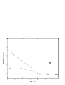
Figure 1: Comparison of the Si accelerations obtained by the light-GLAM method and the MM method (Eq. (13)). The logarithm of $g_{GLAM}^{rad}/{g_{MM}^{rad}}$ is shown vs. the logarithm of optical depth for a model with $T_{\rm eff}=12000\,K$, $\log g=4.00$. The dashed line pertains to 0 Gauss, the solid line to 10000 Gauss.

According to the study by GLAM, one expects to have large discrepancies between the MM and the light-GLAM methods, and we confirm this trend. In Fig. 1 we present the logarithm of the ratio of the accelerations light-GLAM vs. MM for silicon (to be discussed in some detail in Sect. 5.3). The discrepancy is especially strong in the magnetic case and for layers with optical depth smaller than unity. We carried out such a comparison for all the 28 elements investigated, and found that the discrepancy is much smaller for some of them, but larger for some others. The elements for which the discrepancies are smaller than 0.3 dex in the non-magnetic case are: Be, B, Ca, Sc, Ti, V, Cr, Mn, Fe, Co, Ni, Cu. The discrepancies are generally larger in the magnetic case. We do not notice obvious systematic trends except that MM is larger than light-GLAM for noble gases (Ne, Ar) and that MM is smaller than light-GLAM for the alkali elements (Na, K), i.e. elements with a noble gas configuration in their first ionisation stage. This reveals the role of the distribution of energy levels, since levels are not considered in the same way in light-GLAM and in MM. Silicon appears to be a rather typical case concerning the discrepancy between the MM and the light-GLAM methods; we discuss it in more detail. Figure 1 shows that in the non-magnetic case, the MM acceleration of Si is smaller by 0.66 dex, which is the same order of magnitude as the discrepancy found by GLAM for carbon – their discrepancy, however, goes in the opposite direction, their MM acceleration being stronger. Notice that we cannot compare our results concerning carbon with those of GLAM since their computations apply to a star with $T_{\rm eff}=8000\,K$ and to deep layers (outside the validity domain of CARAT). To better understand the reasons for such large differences, we examined the contributions of the various terms entering both methods in detail, especially for the neutral state since it plays a major role in momentum redistribution as already mentioned in Sect. 2.2. The light-GLAM method assumes that ionisation is dominated by transitions to the continuum from high energy levels, because after absorption of a photon leading to a sufficiently high-lying energy level, collisional excitations prevent de-excitation. For the MM method, we have considered the total direct ionisation rate from any level (see Eq.(28)), without taking the added path of excitation collisions before ionisation into account. The MM method thus gives too much weight to low energy levels. If one considers that the MM method underestimates the redistribution of momentum from the neutral to the first ionisation state, one is led to conclude that it gives an upper limit of the radiative acceleration. On the other hand, the light-GLAM method is certainly less justified in the upper atmosphere, where collisional excitations decrease with density, while photoionisation remains efficient. We checked this last argument by comparing the average ionisation rates from low levels (below $2/3$ of the ionisation potential) with those from higher levels, but the final word will come from the detailed analysis of ionisation times, level by level, and using a detailed method like the one of Proffitt et al. (pro99 (1999)), which will be done in future work.

Clearly, we are confronted with a serious dilemma: which method to choose when they yield such different results without a definitive argument in favour of one or the other? It seems reasonable to consider that the MM method gives an upper limit of the radiative acceleration; however, when it becomes larger than the acceleration given by the light-GLAM method, the correct acceleration should lie somewhere in between. To compute the diffusion velocities used in the next subsections, we thus decided to use $g_{i}^{rad}$ values given by the minimum of the respective MM acceleration and of the geometrical mean of the acceleration obtained by both methods:

$$g_{i}^{rad}={\rm{Min}}\left({g_{MM,i}^{rad},\sqrt{g_{MM,i}^{rad}\cdot g_{GLAM,i}^{rad}}\;}\right)$$ (18)

where $g_{MM,i}^{rad}$ and $g_{GLAM,i}^{rad}$ stand for the radiative accelerations obtained by the respective methods.

Figure 2: Logarithm of the rates of abundance increase (per year) vs. logarithm of the optical depth (at 5000 Å) for a horizontal magnetic field ($90\,\degr$). All plots have the same scale as the one in the bottom left corner. Solid lines pertain to $20000\,G$, dashed lines to $10000\,G$, and dotted lines to $0\,G$.

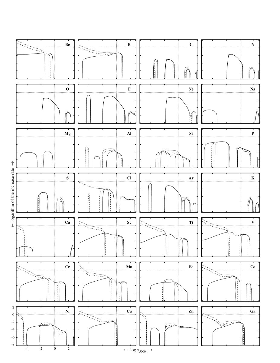
Figure 3: Same as Fig. 2 but for a magnetic field of $20000\,G$ with various inclinations, viz. $90\,\degr$ (solid lines), $60\,\degr$ (dashed lines), and $0\,\degr$ (dotted lines).

5.2 Estimates of stratification trends

The respective rates of abundance increase for each element are presented in Figs. 2 and 3. The curves show the logarithm of $a_{0}(cgs)\times 3.1556\cdot 10^{7}$ (secs) which is the abundance change in one year ($a_{0}$ is given by Eq. (12)). We have plotted this quantity only for positive values of $a_{0}$. Interpreting the curves physically, one could say that they give the amount by which the abundance of the element considered is increased in one year of continuous diffusion. Implicitly we assume that the accelerations remain constant during this time since we use $a_{0}$ for a linear extrapolation of the abundance changes by simply multiplying with $\Delta t$. This is of course a rough approximation; it is known that the accelerations decrease non-linearly with increasing abundances when lines are saturated. Furthermore, we have not considered any boundary conditions here as has to be done when solving the continuity equation. Therefore the curves presented here merely display initial trends in abundance increases. In other words, when the plotted rate is equal to unity at a given depth, this means that the abundance of element $A$ is doubled at that depth in one year of diffusion. One could also consider Figs. 2 and 3 as giving an approximate picture of the accumulation of the various elements in the atmosphere after one year of diffusion.

Note that if the flux derivative is positive, the trend in abundance changes can be positive even in places where elements are not supported. This corresponds to the accumulation of falling particles. Possibly, that kind of accumulation will not survive in any fully time-dependent calculation.

The holes correspond to places where the abundance decreases. Assuming that the abundance stratification process tends to a stationary solution ($a_{\infty}\to 0$), which still has to be demonstrated, a much better prediction of element accumulations can be obtained through an iterative procedure where the accelerations are recomputed after each iteration with updated abundance values (see Hui Bon Hoa et al. hbh02 (2002)); this is, however, outside the scope of the present work.

Figure 2 shows the rates of abundance changes for 2 different values of a horizontal magnetic field (10000 G and 20000 G), as well as the zero field case (angle-independent). For some elements, the rates of abundance changes seem to be completely insensitive to the magnetic field. This is due to the fact that these elements, according to our atomic data, experience radiative accelerations mainly through b-b absorptions in the neutral state. Therefore the diffusion velocity is dominated by the neutral term in Eq. 7 for which $f_{slow,0}=1$ holds exactly. This is, so far, the only systematic behaviour we have been able to clearly identify. For other elements, trends in accumulations are highly sensitive to magnetic field strength and orientation through $f_{slow,i}$ and $\theta$ in Eqs. (7) and (8). As shown in Fig. 3, for a given magnetic field of 20000 G, many elements exhibit significantly different accumulations at the magnetic poles and equators: the thickness of the respective accumulation zones (or element clouds) often appears to be more uniform and larger near the equators than near the poles. Keep in mind that the differences between the dotted lines of Fig. 2 and Fig. 3 can only be due to Zeeman amplification. We note that $a_{0}$, which depends on the derivative of the diffusion fluxes, is not very sensitive to the effect of Zeeman amplification on the accelerations. This is because Zeeman amplifications are more efficient in changing the maximum overabundance of those elements that can be supported by the radiation field than in changing the spatial derivatives of the accelerations (in Eq.(12)). Although we expect the final amount of accumulations for each element to depend much more significantly on Zeeman amplifications, we cannot demonstrate this effect at present since, as mentioned above, we extrapolate the $a_{0}$ in a linear way.

5.3 The silicon case

At this point it is tempting to examine what happens to silicon and to compare these first results to the peculiar behaviour of Si discussed in Sect. 4.1. According to Figs. 2 and 3, a cloud of Si starts to form above $\tau\approx 10^{-2}$ in the magnetic case; in the non-magnetic case, Si starts to accumulate between $\tau\approx 10^{-2}$ and $\tau\approx 10$. This is apparently at variance with Vauclair et al. (vhp79 (1979)), who predict that Si does not accumulate in the zero field case (or in a vertical magnetic field) but will accumulate only when a horizontal magnetic field is present.

To understand this unexpected result we carried out some additional computations assuming 10 times more silicon than in the solar case (adopting 7.55 for the logarithmic Si solar abundance on a scale where the hydrogen abundance is 12). Figure 4 displays the relevant data for the analysis of the behaviour of Si. Panel (a) shows the radiative accelerations, according to Eqs. (13) and (18). Our radiative accelerations are slightly stronger around $\tau=1$ than those of Vauclair et al. (vhp79 (1979) (their Fig.2c) for 0 G, and closer to those of Alecian & Vauclair alv81 (1981) (their Fig.1a). These differences are not surprising since our atomic data and our radiative transfer calculations are much more accurate. As predicted, due to the presence of a horizontal magnetic field, more Si can be supported than without a magnetic field for $\tau\approx 10^{-2}$, but the radiative accelerations remain smaller than gravity for $\tau<1$. Silicon enhanced 10 times is not at all supported by the radiation field throughout the atmosphere at 0 G; despite somewhat higher acceleration values above $\tau\approx 10^{-1}$, this also remains true for the 10 kG case. Considering the diffusion flux (according to Eq. (10)) of silicon in panel (b), one can readily verify that the fluxes are positive in places where the radiative accelerations exceed gravity ($\log g=4.0$). For the magnetic case, diffusion fluxes go to zero at small optical depths. This can be explained by the strong decrease, above $\tau\approx 1$, of the average diffusion coefficient $\left\langle D\right\rangle$ in the magnetic case with $\cos\theta=0$, as shown in panel (c) – the relative populations of the Si ions are displayed in panel (d). The presence of neutrals mitigates this decrease, but not enough to prevent the rather strong decrease in $\left\langle D\right\rangle$ due to ions.

One can conclude that Si is better supported above $\tau\approx 0.1$ by the radiation field in places where the magnetic field lines are horizontal, but less clearly than was predicted by Vauclair et al. (vhp79 (1979)). The total radiative acceleration is less enhanced by the magnetic field than expected, and our results reveal that Si could also be slightly overabundant in places where the magnetic field is vertical (or zero). On the other hand, we have to point out the limits of the “$a_{0}\times\Delta t$” linear analysis carried out in this paper, since the complex Si behaviour is not revealed in Figs. 2 and 3.

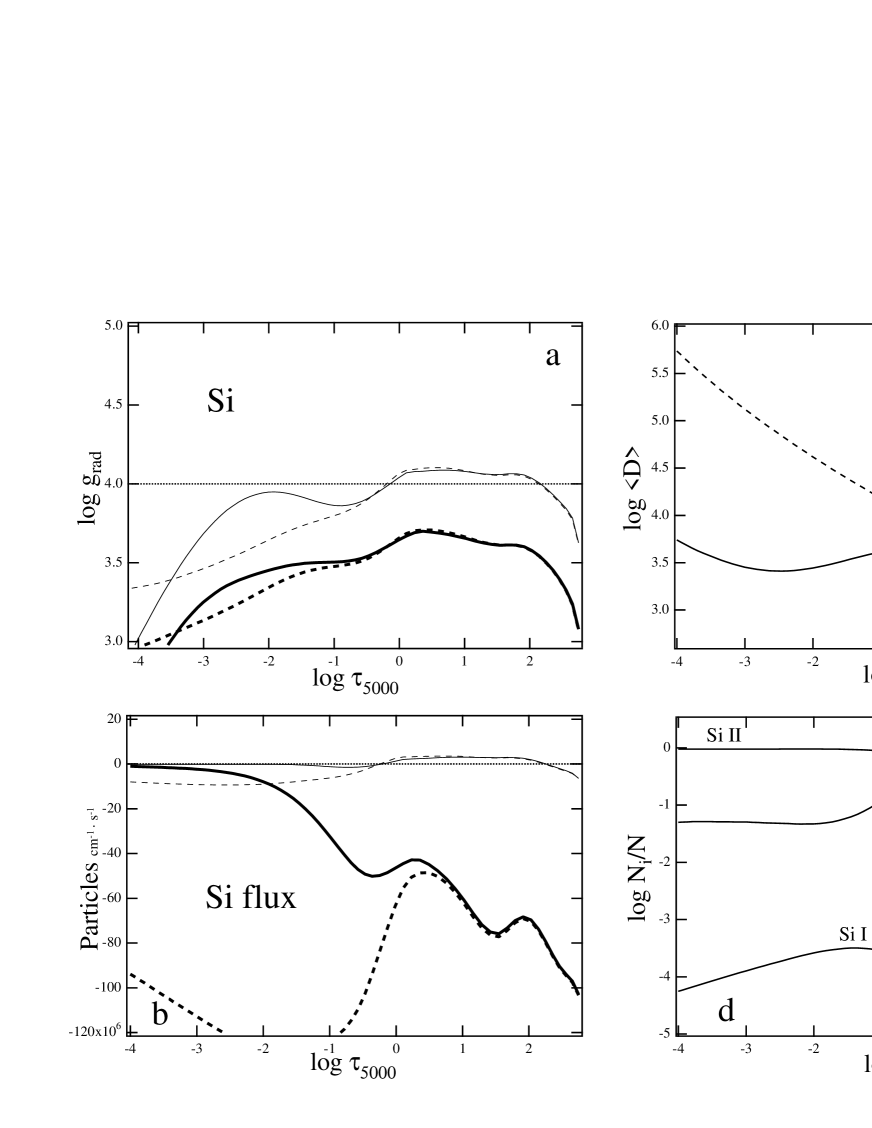
Figure 4: Detailed results for silicon. The dashed lines pertain to 0 G, the solid lines to 10000 G (horizontal). The thin lines are for solar silicon abundance, the heavy lines for a 1 dex overabundance (panels (a) and (b)). Panel (a): Radiative acceleration of Si (Eq. (18)). Panel (b): Diffusion flux of Si (Eq. (10)). Panel (c): Average diffusion coefficient $\left\langle D\right\rangle=\sum{N_{i}f_{slow,i}D_{i}\,/\,N}$ for horizontal magnetic fields ($\cos\theta=0$). Panel (d): Relative populations of the first five Si ions.

6 Conclusions

For this study we have significantly increased the amount of physical processes included in the CARAT code. We added the radiative accelerations due to bound-free transitions by using detailed b-f transition cross sections (whenever available), we added the computation of detailed ionisation/recombination rates, and took the momentum redistribution among ions into account. This has allowed us to obtain results of higher astrophysical relevance than just radiative accelerations. We are now able to calculate diffusion velocities (and particle fluxes) in the presence of magnetic fields at arbitrary angles. Finally we estimated and discussed abundance stratification trends in magnetic Ap stars.

After our previous study of the magnetic amplification of radiative accelerations, this work constitutes a second step towards the modelling of abundance stratifications in CP stars. Several further steps are still necessary to reach that final goal, the most critical of them being an improvement in the theory of momentum redistribution among ions. The use of Eq. (18) is unsatisfactory, at least for elements for which large discrepancies are found between the light-GLAM and the MM methods (see Sect. 5.1). We thus plan to apply a detailed GLAM method following Proffitt et al. (pro99 (1999)) but adapted to the magnetic case, which will become possible thanks to a forthcoming NLTE version of CARAT. In order to study tepid chemically peculiar stars where neutral hydrogen cannot be neglected, we plan to implement ambipolar diffusion in CARAT. A good estimate of final abundance stratifications requires more than simple linear extrapolation of diffusion fluxes, since radiative accelerations depend non-linearly on chemical abundances and on the element fluxes at the boundaries (ingoing and outgoing particles at the top/bottom of the atmosphere). Assuming that a unique stationary solution exists in static atmospheres, an iterative method will converge towards that solution, but in the absence of a unique and/or stationary solution, only the simultaneous time-dependent solution of the continuity equation will allow us to find the correct solution.

Appendix A The redistribution of momentum, the “MM” method

The collision time for ions can be defined as the time required for a deflection by $\pi/2$ through collisions with the other particles in the medium (mainly protons). This collision time is related to the diffusion coefficient (Spitzer spi68 (1968)) by:

$$t_{i}=\frac{{A_{i}\,m_{p}}}{{kT}}\;D_{i},$$ (19)

where $D_{i}$ is the diffusion coefficient of the ion $i$ (presented in more detail in Sect. 4), $A_{i}\,m_{\rm p}$ the mass $({\rm cgs})$ of the ion, and $T,k$ are the temperature and the Boltzmann constant, respectively.

Let $\beta_{col,i}$ be the collision rate defined as $t_{i}^{-1}$. Let $\beta_{ion,i}$ and $\beta_{rec,i}$ be the respective ionisation and recombination rates (see Appendix C). The total interaction rate $\beta_{tot,i}$ is then defined as $\beta_{col,i}+\beta_{ion,i}+\beta_{rec,i}$.

According to the redistribution model proposed by MM, and limiting the redistribution of momentum to only the adjacent ionisation stages (we used the expressions proposed by Alecian & Vauclair ale83 (1983)), the average redistributed radiative acceleration of $A^{0}$ and $A^{+i}$ (for $i>0$) may be written as:

$$g_{0}^{rad}\approx g_{bb,0}\,\frac{{\beta_{col,0}}}{{\beta_{tot,0}}}+g_{A^{+1}}\,\frac{{N_{1}}}{{N_{0}}}\frac{{\beta_{rec,1}}}{{\beta_{tot,1}}}\frac{{\beta_{col,0}}}{{\beta_{tot,0}}},$$ (20)

$$g_{i}^{rad} \approx g_{A^{+(i-1)}}{{N_{i-1}}\,\over{N_{i}}}{{\beta_{ion,i-1}}\over{\beta_{tot,i-1}}}{{\beta_{col,i}}\over{\beta_{tot,i}}}+g_{A^{+i}}\,{{\beta_{col,i}}\over{\beta_{tot,i}}}$$ (21)

$$+\,g_{A^{+(i+1)}}{{N_{i+1}}\over{N_{i}}}{{\beta_{rec,i+1}}\over{\beta_{tot,i+1}}}{{\beta_{col,i}}\over{\beta_{tot,i}}},$$

where $g_{A^{+i}}=g_{bb,i}+g_{bf,i}$ (see Sect. 2.1).

Appendix B The redistribution of momentum, the “light-GLAM” method

In this method discussed in Sect. 2.2, one defines an energy segregation threshold such that all the momentum gained through a b-b transition of $A^{+i}$ is kept by the ion when the energy of the higher level is lower than a given value (here $2/3$ of the ionisation potential). We denote the corresponding acceleration by ${g^{\prime}}_{bb,i}$. The momentum gained through absorption from higher energy levels is entirely given to the ion $A^{+(i+1)}$, and the corresponding acceleration is denoted by ${g^{\prime\prime}}_{bb,i}$. The average redistributed radiative acceleration of $A^{0}$ and $A^{+i}$ (for $i>0$) using the light-GLAM method may then be written as:

$$g_{0}^{rad}\approx g^{\prime}_{bb,0},$$ (22)

$$g_{i}^{rad}\approx{{N_{i-1}}\over{N_{i}}}\,{g^{\prime\prime}}_{bb,i-1}+{g^{\prime}}_{bb,i}+g_{bf,i}.$$ (23)

Appendix C The ionisation and recombination rates

The direct photoionisation rate for ion $A^{+i}$, in level $k$, per atom is (Mihalas mih78 (1978)):

$$R_{ik}=4\,\pi\int_{\nu_{0}}^{\infty}\frac{\alpha_{\nu}J_{\nu}\,d{\nu}}{h{\nu}}$$ (24)

where $\alpha_{\nu}$ denotes the photoionisation cross section, $J_{\nu}$ the mean intensity of radiation, $h$ the Planck constant, and ${\nu_{0}}$ the frequency of the photoionisation edge. In LTE, $J_{\nu}$ corresponds to the Planck function $B_{\nu}$.

The radiative recombination rate per atom can be derived from detailed balancing arguments and we write

$$R_{ki}=4\,\pi\int_{\nu_{0}}^{\infty}\frac{\alpha_{\nu}}{h{\nu}}\left(2h{\nu}^{3}/c^{2}+J_{\nu}\right)e^{-h{\nu}/kT}d{\nu}.$$ (25)

Approximate collisional ionisation rates based on photoionisation cross sections are given by

$$C_{ik}=1.55\,10^{13}\,N_{e}\,T^{-1/2}\,g_{i}\,\alpha({\nu_{0}})\,\exp(-u_{0})/u_{0}$$ (26)

where $N_{e}$ is the electron density, $\alpha({\nu_{0}})$ the threshold photoionisation cross section, and $u_{0}=h{\nu_{0}}/kT$ (see Mihalas mih78 (1978)). For the parameter $g_{i}$, we follow Seaton (2005, private communication) and assume $g_{0}=0.07,g_{i}=0.25$ (for $i>0$). Again, detailed balancing arguments can be applied to obtain the downward rate as

$$C_{ki}=(N_{i}/N_{j})^{*}C_{ik},$$ (27)

where the asterisk denotes LTE values.

The ionisation rate of Appendix A is then given by:

$$\beta_{ion,i}=\frac{1}{{N_{i}}}\sum\limits_{k}{N_{ik}\left({R_{ik}+C_{ik}}\right)}$$ (28)

The recombination rate has been evaluated assuming LTE as in Hui-Bon-Hoa et al. (hui96 (1996)).