Primordial Non-Gaussianity and Analytical Formula for
Minkowski Functionals of the Cosmic Microwave Background
and Large-scale Structure

Abstract

We derive analytical formulae for the Minkowski Functions of the cosmic microwave background (CMB) and large-scale structure (LSS) from primordial non-Gaussianity. These formulae enable us to estimate a non-linear coupling parameter, $f_{\rm NL}$, directly from the CMB and LSS data without relying on numerical simulations of non-Gaussian primordial fluctuations. One can use these formulae to estimate statistical errors on $f_{\rm NL}$ from Gaussian realizations, which are much faster to generate than non-Gaussian ones, fully taking into account the cosmic/sampling variance, beam smearing, survey mask, etc. We show that the CMB data from the Wilkinson Microwave Anisotropy Probe should be sensitive to $|f_{\rm NL}|\simeq 40$ at the $68\%$ confidence level. The Planck data should be sensitive to $|f_{\rm NL}|\simeq 20$. As for the LSS data, the late-time non-Gaussianity arising from gravitational instability and galaxy biasing makes it more challenging to detect primordial non-Gaussianity at low redshifts. The late-time effects obscure the primordial signals at small spatial scales. High-redshift galaxy surveys at $z>2$ covering $\sim 10$ Gpc³ volume would be required for the LSS data to detect $|f_{\rm NL}|\simeq 100$. Minkowski Functionals are nicely complementary to the bispectrum because the Minkowski Functionals are defined in real space and the bispectrum is defined in Fourier space. This property makes the Minkowski Functionals a useful tool in the presence of real-world issues such as anisotropic noise, foreground and survey masks. Our formalism can be extended to scale-dependent $f_{\rm NL}$ easily.

Received 2006 July 12; accepted 2006 August 22

1 Introduction

Recent observations of cosmological fluctuations from the Cosmic Microwave Background (CMB) and Large Scale Structure (LSS) strongly support basic predictions of inflationary scenarios: primordial fluctuations are nearly scale-invariant (Spergel et al., 2003; Tegmark et al., 2004; Seljak et al., 2005; Spergel et al., 2006), adiabatic (Peiris et al., 2003; Bucher et al., 2004; Bean et al., 2006), and Gaussian (Komatsu et al., 2002, 2003; Creminelli et al., 2006; Spergel et al., 2006, and references therein). In order to discriminate between more-than-100 candidate inflationary models, however, one needs to look for deviations from the scale-invariance, adiabaticity as well as Gaussianity, for which different inflationary models make specific predictions. Inflationary models based upon a slowly rolling single-field scalar field generally predict very small deviations from Gaussianity; however, the post-inflationary evolution of non-linear metric perturbations inevitably generates ubiquitous non-Gaussian fluctuations. On the other hand, a broad class of inflationary models based upon different assumptions about the nature of scalar field(s) can generate significant primordial non-Gaussianity (Lyth et al., 2003; Dvali et al., 2004; Arkami-Hamed et al., 2004; Alishahiha et al., 2004; Bartolo et al., 2004). Therefore, Gaussianity of the primordial fluctuations offers a direct test of inflationary models.

It is customary to adopt the following simple form of primordial non-Gaussianity in Bardeen’s curvature perturbations during the matter era (e.g., Komatsu & Spergel, 2001):

$$\Phi=\phi+f_{\rm NL}(\phi^{2}-\langle\phi^{2}\rangle),$$ (1)

where $\phi$ is an auxiliary random-Gaussian field and $f_{\rm NL}$ characterizes the amplitude of a quadratic correction to the curvature perturbations. Note that $\Phi$ is related to the primordial comoving curvature perturbations generated during inflation, ${\cal R}$, by $\Phi=(3/5){\cal R}$. While this quadratic form is motivated by inflationary models based upon a single slowly-rolling scalar field, the actual predictions usually include momentum dependence in $f_{\rm NL}$. (That is to say, $f_{\rm NL}$ is not a constant.) Therefore, when precision is required, one should use the actual formula given by specific processes, either from primordial non-Gaussianity from inflation or the post-inflationary evolution of non-linear perturbations, to calculate a more accurate form of statistical quantities such as the angular bispectrum of CMB (Babich et al., 2004; Liguori et al., 2006). Nevertheless, a constant $f_{\rm NL}$ is still a useful parameterization of non-Gaussianity which enables us to obtain simple analytical formulae for the statistical quantities to compare with observations. The use of a constant $f_{\rm NL}$ is also justified by the fact that the current observations are not sensitive enough to detect momentum-dependence of $f_{\rm NL}$. Therefore, we adopt the constant $f_{\rm NL}$ for our analysis throughout this paper. Note that it is actually straightforward to extend our formalism to a momentum-dependent $f_{\rm NL}$.

So far, analytical formulae for the statistical quantities of the CMB from primordial non-Gaussianity are known only for the angular bispectrum (Komatsu & Spergel, 2001; Babich & Zaldarriaga, 2004; Liguori et al., 2006) and trispectrum (Okamoto & Hu, 2002; Kogo & Komatsu, 2006). The analytical formulae are extremely valuable especially when one tries to measure non-Gaussian signals from the data. Fast, nearly optimal estimators for $f_{\rm NL}$ have been derived on the basis of these analytical formulae (Komatsu et al., 2005; Creminelli et al., 2006), and have been successfully applied to the CMB data from the Wilkinson Microwave Anisotropy Probe (WMAP): the current constraint on $f_{\rm NL}$ from the angular bispectrum is $-54$ to $114$ at the 95% confidence level (Komatsu et al., 2003; Spergel et al., 2006). (See Creminelli et al., 2006, for an alternative parameterization of $f_{\rm NL}$.) As for the LSS, the analytical formula is known only for the 3-d bispectrum (Verde et al., 2000; Scoccimarro et al., 2004). The LSS bispectrum contains not only the primordial non-Gaussianity, but also the late-time non-Gaussianity from gravitational instability and galaxy biasing, which potentially obscure the primordial signatures.

In this paper, we derive analytical formulae for another statistical tool, namely the Minkowski Functionals (MFs), which describe morphological properties of fluctuating fields (Mecke et al., 1994; Schmalzing & Buchert, 1997; Schmalzing & G$\acute{\rm o}$rski, 1998; Winitzki & Kosowsky, 1998). In $d$-dimensional space ($d=2$ for CMB and $d=3$ for LSS), $d+1$ MFs are defined, as listed in Table 1. The “Euler characteristic” measures topology of the fields, and is essentially given by the number of hot spots minus the number of cold spots when $d=2$. This quantity is sometimes called the “genus statistics”, which was independently re-discovered by Gott et al. (1986) in search of a topological measure of non-Gaussianity in the cosmic density fields. (The Euler characteristic and genus are different only by a numerical coefficient, $-1/2$.)

Table 1: Minkowski Functionals defined in $d-$dimensional space: $d=2$ for CMB and $d=3$ for LSS.

observations	$d$	$V_{0}$	$V_{1}$	$V_{2}$	$V_{3}$
CMB	2	Area	Total Circumference	Euler Characteristic	–
LSS	3	Volume	Surface Area	Total Mean Curvature	Euler Characteristic

Why study MFs? Since different statistical methods are sensitive to different aspects of non-Gaussianity, one should study as many statistical methods as possible. Most importantly, the MFs and bispectrum are very different in that MFs are defined in real space, whereas the bispectrum is defined in Fourier (or harmonic) space. Therefore, these statistical methods are nicely complementary to each other. Previously there are several attempts to give constraints on the primordial non-Gaussianity using MFs (e.g, Novikov et al., 2000). Although we shall show in this paper that the MFs do not contain information more than the bispectrum in the limit that non-Gaussianity is weak, the complementarity is still powerful in the presence of complicated real-world issues such as inhomogeneous noise, survey mask, foreground contamination, etc. The MFs have also been used to constrain $f_{\rm NL}$. Komatsu et al. (2003) and Spergel et al. (2006) have used numerical simulations of non-Gaussian CMB sky maps to calculate the predicted form of MFs as a function of $f_{\rm NL}$, and compared the predictions with the WMAP data to constrain $f_{\rm NL}$, obtaining similar constraints to the bispectrum ones. This method (calculating the form of MFs from non-Gaussian simulations) is, however, a painstaking process: it takes about three hours to simulate one non-Gaussian map on one processor of SGI Origin 300. When cosmological parameters are varied, one needs to re-simulate a whole batch of non-Gaussian maps from the beginning — this is a highly inefficient approach. Once we have the analytical formula for the MFs as a function of $f_{\rm NL}$, however, we no longer need to simulate non-Gaussian maps, greatly speeding up the measurement of $f_{\rm NL}$ from the data.

We use the perturbative formula for MFs originally derived by Matsubara (1994, 2003): assuming that non-Gaussianity is weak, which has been justified by the current constraints on $f_{\rm NL}$, we consider the lowest-order corrections to the MFs using the multi-dimensional Edgeworth expansion around a Gaussian distribution function.

The organization of paper is as follows; In § 2 we review the generic perturbative formula for the Minkowski Functionals. In § 3 we derive the analytical formula for MFs of the CMB from primordial non-Gaussian fluctuations parameterized by $f_{\rm NL}$. We also estimate projected statistical errors on $f_{\rm NL}$ expected from the WMAP data from multi-year observations as well as from the Planck data. In § 4 we derive the analytical formula for MFs of the LSS from primordial non-Gaussianity, non-linear gravitational evolution, and galaxy biasing in a perturbative manner. § 5 is devoted to summary and conclusions. In Appendix A we outline our method for computing the MFs from the CMB and LSS data. We also describe our simulations of CMB and LSS. In Appendix B we derive the analytical formula for the galaxy bispectrum. In Appendix C we compare the analytical MFs of CMB with non-Gaussian simulations in the Sachs–Wolfe limit. In Appendix D, we extend the corrections of primordial potential to $n$-th order, in order to examine more carefully validity of our perturbative expansion.

Throughout this paper, we assume $\Lambda$CDM cosmology with the cosmological parameters at the maximum likelihood peak from the WMAP first-year data only fit (Spergel et al., 2003). Specifically, we adopt $\Omega_{b}=0.049$, $\Omega_{cdm}=0.271$, $\Omega_{\Lambda}=0.68$, $H_{0}=68.2~{}{\rm km~{}s^{-1}~{}Mpc^{-1}}$, $\tau=0.0987$, and $n_{s}=0.967$. The amplitude of primordial fluctuations has been normalized by the first acoustic peak of the temperature power spectrum, $l(l+1)C_{l}/(2\pi)=(74.7~{}{\mu}{\rm K})^{2}$ at $l=220$ (Page et al., 2003b).

2 General Perturbative Formula for Minkowski Functionals

Suppose that we have a $d$-dimensional fluctuating field, $f$, which has zero mean. Then, one may define the MFs for a given threshold, $\nu\equiv f/\sigma_{0}$, where $\sigma_{0}\equiv\langle f^{2}\rangle^{1/2}$ is the standard deviation of $f$. Matsubara (2003) has obtained the analytical formulae for the $k$-th Minkowski Functionals of weakly non-Gaussian fields in $d$-dimension, $V_{k}^{(d)}(\nu)$, as (Eq. (133) of Matsubara, 2003)

$$V_{k}^{(d)}(\nu) = \frac{1}{(2\pi)^{(k+1)/2}}\frac{\omega_{d}}{\omega_{d-k}\omega_{k}}\left(\frac{\sigma_{1}}{\sqrt{d}\sigma_{0}}\right)^{k}e^{-\nu^{2}/2}\left\{H_{k-1}(\nu)\right.$$ (2)

$$+\left[\frac{1}{6}S^{(0)}H_{k+2}(\nu)+\frac{k}{3}S^{(1)}H_{k}(\nu)\right.$$

$$\left.\left.+\frac{k(k-1)}{6}S^{(2)}H_{k-2}(\nu)\right]\sigma_{0}+{\cal O}(\sigma_{0}^{2})\right\},$$

where $H_{n}(\nu)$ are the Hermite polynomials, and $\omega_{k}\equiv\pi^{k/2}/{\Gamma(k/2+1)}$ gives $\omega_{0}=1$, $\omega_{1}=2$, $\omega_{2}=\pi$, and $\omega_{3}=4\pi/3$. Here, $S^{(i)}$ are the “skewness parameters” defined by

$$S^{(0)} \equiv \frac{\langle f^{3}\rangle}{\sigma_{0}^{4}},$$ (3)

$$S^{(1)} \equiv -\frac{3}{4}\frac{\langle f^{2}(\nabla^{2}f)\rangle}{\sigma_{0}^{2}\sigma_{1}^{2}},$$ (4)

$$S^{(2)} \equiv -\frac{3d}{2(d-1)}\frac{\langle(\nabla f)\cdot(\nabla f)(\nabla^{2}f)\rangle}{\sigma_{1}^{4}},$$ (5)

which characterize the skewness of fluctuating fields and their derivatives. The quantity $\sigma_{i}$ characterizes the variance of fluctuating fields and their derivatives, and is given by

$$\sigma_{j}^{2}\equiv\int_{0}^{\infty}\frac{k^{2}dk}{2\pi^{2}}k^{2j}P(k)W^{2}(kR),$$ (6)

for $d=3$, and

$$\sigma_{j}^{2}\equiv\frac{1}{4\pi}\sum_{l}(2l+1)\left[l(l+1)\right]^{j}C_{l}W^{2}_{l},$$ (7)

for $d=2$. In both cases $W$ represents a smoothing kernel, or a window function, which will be given by a product of the experimental beam transfer function, pixelization window function, and an extra Gaussian smoothing. The power spectra, $P(k)$ for $d=3$ and $C_{l}$ for $d=2$, are defined as

$$\langle\tilde{f}_{\mathbf{k}}\tilde{f}^{*}_{{\mathbf{k}}^{\prime}}\rangle = (2\pi)^{3}P(k)\delta_{D}({\mathbf{k}}-{\mathbf{k}}^{\prime}),$$ (8)

$$\langle a_{lm}a_{l^{\prime}m^{\prime}}^{*}\rangle = C_{l}\delta_{ll^{\prime}}\delta_{mm^{\prime}},$$ (9)

where $\delta_{D}({\mathbf{k}})$ is the Dirac delta function, and the Fourier and harmonic coefficients are given by

$$f({\mathbf{x}})=\int\frac{d^{3}{\mathbf{k}}}{(2\pi)^{3}}\tilde{f}_{\mathbf{k}}e^{i{\mathbf{k}}\cdot{\mathbf{x}}},$$ (10)

$$f({\mathbf{\Omega}})=\sum_{lm}a_{lm}Y_{lm}({\mathbf{\Omega}}),$$ (11)

for $d=3$ and 2, respectively. Finally, the most relevant Hermite polynomials are given by

$$H_{-1}(\nu) = \sqrt{\frac{\pi}{2}}e^{\nu^{2}/2}{\rm erfc}\left(\frac{\nu}{\sqrt{2}}\right),$$ (12)

$$H_{0} = 1,$$ (13)

$$H_{1}(\nu) = \nu,$$ (14)

$$H_{2}(\nu) = \nu^{2}-1,$$ (15)

$$H_{3}(\nu) = \nu^{3}-3\nu,$$ (16)

$$H_{4}(\nu) = \nu^{4}-6\nu^{2}+3,$$ (17)

$$H_{5}(\nu) = \nu^{5}-10\nu^{3}+15\nu.$$ (18)

3 Application I: Cosmic Microwave Background

3.1 Analytical Formula for Minkowski Functionals of CMB

For the cosmic microwave background, we have $d=2$ and $f=\Delta T/T$. We define the angular bispectrum as

$$B_{l_{1}l_{2}l_{3}}^{m_{1}m_{2}m_{3}}\equiv\langle a_{l_{1}m_{1}}a_{l_{2}m_{2}}a_{l_{3}m_{3}}\rangle.$$ (19)

Then, by expanding skewness parameters into spherical harmonics, we obtain

$$S^{(0)} = \frac{1}{4\pi\sigma_{0}^{4}}\sum_{l_{i}m_{i}}B_{l_{1}l_{2}l_{3}}^{m_{1}m_{2}m_{3}}{\cal G}_{l_{1}l_{2}l_{3}}^{m_{1}m_{2}m_{3}}W_{l_{1}}W_{l_{2}}W_{l_{3}},$$ (20)

$$S^{(1)} = \frac{3}{16\pi\sigma_{0}^{2}\sigma_{1}^{2}}\sum_{l_{i}m_{i}}\frac{l_{1}(l_{1}+1)+l_{2}(l_{2}+1)+l_{3}(l_{3}+1)}{3}$$ (21)

$$\times B_{l_{1}l_{2}l_{3}}^{m_{1}m_{2}m_{3}}{\cal G}_{l_{1}l_{2}l_{3}}^{m_{1}m_{2}m_{3}}W_{l_{1}}W_{l_{2}}W_{l_{3}},$$

$$S^{(2)} = \frac{3}{8\pi\sigma_{1}^{4}}\sum_{l_{i}m_{i}}\left\{\frac{\left[l_{1}(l_{1}+1)+l_{2}(l_{2}+1)-l_{3}(l_{3}+1)\right]}{3}\right.$$ (22)

$$\left.\times l_{3}(l_{3}+1)+({\rm cyc.})\right\}B_{l_{1}l_{2}l_{3}}^{m_{1}m_{2}m_{3}}{\cal G}_{l_{1}l_{2}l_{3}}^{m_{1}m_{2}m_{3}}$$

$$\times W_{l_{1}}W_{l_{2}}W_{l_{3}},$$

where (cyc.) means the addition of terms with the same cyclic order of the subscripts as the previous term, $W_{l}$ is a smoothing kernel in $l$ space and ${\cal G}_{l_{1}l_{2}l_{3}}^{m_{1}m_{2}m_{3}}$ is the Gaunt integral,

$${\cal G}_{l_{1}l_{2}l_{3}}^{m_{1}m_{2}m_{3}}\equiv\int d\hat{\mathbf{n}}~{}Y_{l_{1}m_{1}}(\hat{\mathbf{n}})Y_{l_{2}m_{2}}(\hat{\mathbf{n}})Y_{l_{3}m_{3}}(\hat{\mathbf{n}}).$$ (23)

Note that we have used the following properties of $Y_{lm}(\hat{\mathbf{n}})$:

$$\nabla^{2} Y_{lm}(\hat{\mathbf{n}})=-l(l+1)Y_{lm}(\hat{\mathbf{n}}),$$ (24)

$$\int d\hat{\mathbf{n}} \left[\nabla Y_{l_{1}m_{1}}(\hat{\mathbf{n}})\right]\cdot\left[\nabla Y_{l_{2}m_{2}}(\hat{\mathbf{n}})\right]Y_{l_{3}m_{3}}(\hat{\mathbf{n}})$$ (25)

$$= \frac{l_{1}(l_{1}+1)+l_{2}(l_{2}+1)-l_{3}(l_{3}+1)}{2}{\cal G}_{l_{1}l_{2}l_{3}}^{m_{1}m_{2}m_{3}}.$$

The summation over $m_{i}$ can be done by writing

$$B_{l_{1}l_{2}l_{3}}^{m_{1}m_{2}m_{3}}={\cal G}_{l_{1}l_{2}l_{3}}^{m_{1}m_{2}m_{3}}b_{l_{1}l_{2}l_{3}},$$ (26)

where $b_{l_{1}l_{2}l_{3}}$ is the reduced bispectrum that depends on specific non-Gaussian models (Komatsu & Spergel, 2001). Using the reduced bispectrum, we finally obtain the analytical formula for MFs of the CMB:

$$S^{(0)} = \frac{3}{2\pi\sigma_{0}^{4}}\sum_{2\leq l_{1}\leq l_{2}\leq l_{3}}I^{2}_{l_{1}l_{2}l_{3}}b_{l_{1}l_{2}l_{3}}W_{l_{1}}W_{l_{2}}W_{l_{3}},$$ (27)

$$S^{(1)} = \frac{3}{8\pi\sigma_{0}^{2}\sigma_{1}^{2}}\sum_{2\leq l_{1}\leq l_{2}\leq l_{3}}\left[l_{1}(l_{1}+1)+l_{2}(l_{2}+1)+l_{3}(l_{3}+1)\right]$$ (28)

$$\times I^{2}_{l_{1}l_{2}l_{3}}b_{l_{1}l_{2}l_{3}}W_{l_{1}}W_{l_{2}}W_{l_{3}},$$

$$S^{(2)} = \frac{3}{4\pi\sigma_{1}^{4}}\sum_{2\leq l_{1}\leq l_{2}\leq l_{3}}\left\{\left[l_{1}(l_{1}+1)+l_{2}(l_{2}+1)-l_{3}(l_{3}+1)\right]\right.$$ (29)

$$\left.\times l_{3}(l_{3}+1)+({\rm cyc.})\right\}I^{2}_{l_{1}l_{2}l_{3}}b_{l_{1}l_{2}l_{3}}W_{l_{1}}W_{l_{2}}W_{l_{3}},$$

where

$$I_{l_{1}l_{2}l_{3}}\equiv\sqrt{\frac{(2l_{1}+1)(2l_{2}+1)(2l_{3}+1)}{4\pi}}\left(\begin{array}[]{ccc}l_{1}&l_{2}&l_{3}\\ 0&0&0\end{array}\right),$$ (30)

and we have used

$$\sum_{m_{1}m_{2}m_{3}}\left({\cal G}_{l_{1}l_{2}l_{3}}^{m_{1}m_{2}m_{3}}\right)^{2}=I_{l_{1}l_{2}l_{3}}^{2}.$$ (31)

When $f_{\rm NL}$ is a constant, the form of $b_{l_{1}l_{2}l_{3}}$ is given by (Komatsu & Spergel, 2001)

$$b_{l_{1}l_{2}l_{3}} = 2\int^{\infty}_{0}r^{2}dr[b^{L}_{l_{1}}(r)b^{L}_{l_{2}}(r)b^{NL}_{l_{3}}(r)+b^{L}_{l_{1}}(r)b^{NL}_{l_{2}}(r)b^{L}_{l_{3}}(r)$$ (32)

$$+b^{NL}_{l_{1}}(r)b^{L}_{l_{2}}(r)b^{L}_{l_{3}}(r)],$$

where

$$b^{L}_{l}(r)\equiv\frac{2}{\pi}\int^{\infty}_{0}k^{2}dkP_{\phi}(k)g_{Tl}(k)j_{l}(kr),$$ (33)

$$b^{NL}_{l}(r)\equiv\frac{2}{\pi}\int^{\infty}_{0}k^{2}dkf_{NL}g_{Tl}(k)j_{l}(kr),$$ (34)

and $P_{\phi}(k)\propto k^{n_{s}-4}$ is the primordial power spectrum of $\phi$. The amplitude of $P_{\phi}(k)$ is fixed by the first peak amplitude of the temperature power spectrum, $l(l+1)C_{l}/(2\pi)=(74.7~{}\mu{\rm K})^{2}$ at $l=220$ (Page et al., 2003a), and the temperature power spectrum is given by

$$C_{l}=\frac{2}{\pi}\int^{\infty}_{0}k^{2}dkP_{\phi}(k)g_{Tl}^{2}(k).$$ (35)

We calculate the full radiation transfer function, $g_{Tl}(k)$, using the publicly-available CMBFAST code (Seljak & Zaldarriaga, 1996). Note that our formalism is completely generic. One can easily generalize our results to non-Gaussian models with a momentum-dependent $f_{\rm NL}$ by using an appropriate form of $b_{l_{1}l_{2}l_{3}}$ given in Liguori et al. (2006). Our results suggest that the MFs do not contain information beyond the bispectrum when non-Gaussianity is weak. The MFs of CMB basically measure the weighted sum of the CMB angular bispectrum.

In Figure 1, we plot the skewness parameters, $S^{(a)}$ (Eqs. [27–29]), and $S^{(a)}$ multiplied by $\sigma_{0}$, for a pure signal of CMB anisotropy (without noise) as a function of a Gaussian smoothing width, $\theta_{s}$, which determines a Gaussian smoothing kernel, $W_{l}=\exp[-l(l+1)\theta_{s}^{2}/2]$. The perturbative expansion of MFs works only when $S^{(a)}\sigma_{0}$ is much smaller than unity (see Eq. [2]). We find that the perturbative expansion is valid for $f_{\rm NL}\ll 3300$ from the results plotted in the right panel of Figure 1 that show $|S^{(a)}|\sigma_{0}\lesssim 3\times 10^{-4}~{}f_{\rm NL}$.

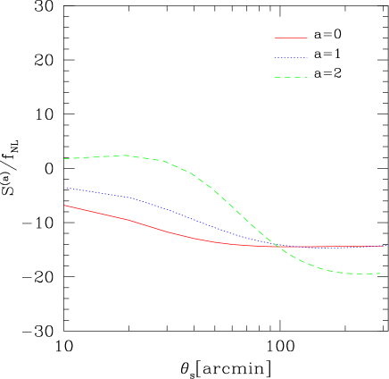
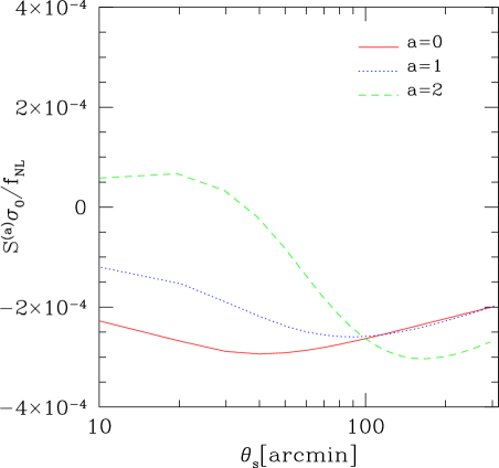
Figure 1: (Left) Skewness parameters, $S^{(a)}$, for $a=0$ (solid), 1 (dotted), and 2 (dashed). (Right) Skewness parameters multiplied by variance, $S^{(a)}\sigma_{0}$, for $a=0$ (solid), 1 (dotted), and 2 (dashed). Both have been divided by $f_{\rm NL}$, and are plotted as a function of a Gaussian smoothing width, $\theta_{s}$. Note that $S^{(2)}$ changes its sign at $\theta_{s}\sim 40$ arcmin.

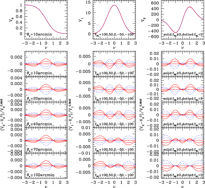
Figure 2: Analytical predictions for the Minkowski Functionals of CMB temperature anisotropy with primordial non-Gaussianity characterized by $f_{\rm NL}=-100$, $-50$ (dotted), 0, 50, and 100 (solid). Each MF, $V_{k}$ ($k=0$, 1, and 2), is plotted in the top panels. The other panels show the difference between non-Gaussian and Gaussian MFs, $V_{k}^{G}$, divided by the maximum amplitude of $V_{k}^{G}$. From the top to bottom, $\theta_{s}=10$, 20, 40, 70, and 100 arcmin are shown.

This Figure also shows how MFs may be as powerful as the angular bispectrum in measuring $f_{\rm NL}$. Komatsu & Spergel (2001) have shown that sensitivity of the first skewness parameter, $S^{(0)}$, to $f_{\rm NL}$ is much worse than that of the angular bispectrum, as acoustic oscillations in $l$ space smear out non-Gaussian signals in the skewness, which is the weighted sum of the angular bispectrum over $l$. (The angular bispectrum is negative in the Sachs-Wolfe regime at low $l$, and oscillates about zero by changing its sign at higher $l$.) The MFs are sensitive to not only $S^{(0)}$, but also $S^{(1)}$ and $S^{(2)}$. The weight of the sum over multipoles differs among three skewness parameters: $S^{(2)}$ has the largest weight at high $l$, $S^{(0)}$ has the largest weight at low $l$, and $S^{(1)}$ is somewhere in between (Eqs. [27–29]). In particular, because $S^{(2)}$ picks up the highest multipoles efficiently, $S^{(2)}$ changes its sign depending on $\theta_{s}$. $S^{(2)}$ is negative on very large angular scales. As $\theta_{s}$ decreases (as the small scale information is included), $S^{(2)}$ increases, and eventually changes its sign to positive values near the scale of the first acoustic peak, $\theta_{s}\sim 40$ arcmin, where the bispectrum has the largest amplitude, while the other two skewness parameters do not change their signs. Therefore, $S^{(2)}$ keeps information about the acoustic oscillations. This property is crucial for obtaining a better signal-to-noise ratio for primordial non-Gaussianity in the CMB.

Figure 2 shows the predicted MFs of CMB temperature anisotropy, $V_{0}$, $V_{1}$ and $V_{2}$, as a function of $f_{\rm NL}$. The MFs for $f_{\rm NL}=100,50$ and $0$ are plotted in the solid lines, while the MFs for $f_{\rm NL}=-50$ and $-100$ are plotted in the dotted lines. The lower panels show the difference between the Gaussian and non-Gaussian MFs divided by the maximum amplitude of Gaussian MFs. Primordial non-Gaussianity with $f_{\rm NL}=100$ changes $V_{0}$, $V_{1}$ and $V_{2}$ by 0.2%, 0.4%, and 1%, respectively, relative to the maximum amplitude of the corresponding Gaussian MFs. While $V_{0}$ (area) has little dependence on $\theta_{s}$, $V_{2}$ (Euler characteristic) depends on $\theta_{s}$ strongly, which is mainly due to the sign change of $S^{(2)}$ at $\theta_{s}\sim 40$ arcmin.

In Appendix C we show that these analytical predictions agree with non-Gaussian simulations in the Sachs–Wolfe limit very well. The comparison with the full simulations that include the full radiation transfer function will be reported elsewhere.

3.2 Measuring $f_{\rm NL}$ from Minkowski Functionals of CMB

The MFs at different threshold values, $\nu$, are correlated, and different MFs are also correlated, i.e.,

$$\Sigma_{kk^{\prime}}^{(d)}(\nu,\nu^{\prime})\equiv\langle V_{k}^{(d)}(\nu)V_{k^{\prime}}^{(d)}(\nu^{\prime})\rangle\neq\delta_{kk^{\prime}}\delta(\nu-\nu^{\prime}).$$ (36)

where $\delta$ denotes the Kronecker delta. Therefore, it is important to use the full covariance matrix, $\Sigma$, in the data analysis. We obtain the full covariance matrix from Monte Carlo simulations of Gaussian temperature anisotropy. Because non-Gaussianity is weak, the covariance matrix estimated from Gaussian simulations is a good approximation of the exact one. In Appendix A.1 we describe our methods for computing MFs from the pixelized CMB maps. In Appendix A.2 and A.3 we describe our methods for simulating sky maps of CMB temperature anisotropy with noise and instrumental characteristics of the WMAP and Planck experiment respectively.

We use the Fisher information matrix formalism to estimate the projected errors on $f_{\rm NL}$ from given measurement errors on MFs. The Fisher matrix, $F_{ij}$, is written in terms of the inverse of the covariance matrix, $\Sigma^{-1}$, as

$$F^{(d)}_{ij}=\sum_{kk^{\prime}}\int d\nu\int d\nu^{\prime}~{}\frac{\partial V^{(d)}_{k}(\nu)}{\partial p_{i}}(\Sigma^{-1})^{(d)}_{kk^{\prime}}(\nu,\nu^{\prime})\frac{\partial V^{(d)}_{k^{\prime}}(\nu^{\prime})}{\partial p_{j}},$$ (37)

where $p_{i}$ is the $i$-th parameter. For CMB, we consider only one parameter, $p_{1}=f_{NL}$, whereas for LSS we also include galaxy biasing parameters (see § 4). The projected 1-$\sigma$ error on $f_{NL}$ is given by the square root of $(F^{-1})_{11}$. While equation (37) may be evaluated for a given smoothing scale, $\theta_{s}$, one will eventually need to combine all combinations of MFs at different $\theta_{s}$ to obtain the best constraint on $f_{\rm NL}$ from given data. The MFs at different $\theta_{s}$ are also correlated. We therefore calculate the full covariance matrix of MFs that consists of $N_{\nu}\times N_{\rm MF}\times N_{\rm s}$ elements, where $N_{\nu}=25$ is the number of bins for $\nu$ per each MF in the range of $\nu$ from $-3$ to $3$, $N_{\rm MF}=3$ and $4$ is the number of MFs for $d=2$ and $3$, respectively (i.e., $N_{\rm MF}=3$ for CMB and $4$ for LSS), and $N_{\rm s}$ is the number of smoothing scales used in the analysis. The Fisher matrix may be written as

$$F^{(d)}_{ij}=\sum_{\alpha\alpha^{\prime}}\frac{\partial V^{(d)}_{\alpha}}{\partial p_{i}}(\Sigma^{-1})^{(d)}_{\alpha\alpha^{\prime}}\frac{\partial V^{(d)}_{\alpha^{\prime}}}{\partial p_{j}},$$ (38)

where $\alpha$ is a single index denoting $k$, $\nu$, and $\theta_{s}$.

Table 2: Projected 1-$\sigma$ errors on $f_{\rm NL}$ from each of the Minkowski Functionals of CMB temperature anisotropy ($V_{0}$: area, $V_{1}$: total circumference, $V_{2}$: Euler characteristic) as well as from the combined analysis of all the Minkowski Functionals, for various combinations of smoothing scales, $\theta_{s}$. We use noise and beam properties of WMAP 1-year and 8-year observations with the $Kp0$ mask. The last block of Table shows the 1-$\sigma$ errors from the “ultimate WMAP”, which uses all sky with zero noise. (The beam smearing is still included.)

	WMAP 1-year		WMAP 8-year		no noise and no sky cut
$\theta_{s}$[arcmin]	All	($V_{0},V_{1},V_{2}$)	All	($V_{0},V_{1},V_{2}$)	All	($V_{0},V_{1},V_{2}$)
$100$	$271$	$(671,297,494)$	$269$	$(668,296,494)$	$135$	$(461,146,182)$
$70$	$153$	$(456,168,272)$	$153$	$(456,168,271)$	$94$	$(363,100,137)$
$40$	$86$	$(283,96,148)$	$84$	$(289,95,144)$	$59$	$(236,67,94)$
$20$	$54$	$(176,67,82)$	$51$	$(183,63,79)$	$41$	$(160,52,62)$
$10$	$73$	$(139,92,91)$	$41$	$(134,54,61)$	$35$	$(120,47,51)$
$5$	—		$75$	$(125,94,87)$	$30$	$(106,42,43)$
$10,20~{}\&~{}40$	$46$	$(92,62,67)$	$36$	$(82,51,56)$	$30$	$(49,43,45)$
$5,10~{}\&~{}20$	—		$36$	$(71,52,53)$	$22$	$(46,32,37)$

Table 3: Same as Table 2 but for Planck data.

	Planck		no noise and no sky cut
$\theta_{s}$[arcmin]	All	($V_{0},V_{1},V_{2}$)	All	($V_{0},V_{1},V_{2}$)
$100$	$271$	$(665,299,502)$	$136$	$(462,147,184)$
$70$	$157$	$(463,171,278)$	$95$	$(354,102,141)$
$40$	$77$	$(281,86,128)$	$54$	$(235,61,84)$
$20$	$46$	$(153,59,69)$	$37$	$(140,49,55)$
$10$	$32$	$(115,45,45)$	$28$	$(102,40,39)$
$5$	$24$	$(97,31,36)$	$21$	$(87,27,30)$
$5,10~{}\&~{}20$	$19$	$(46,26,31)$	$15$	$(38,22,26)$

Let us comment on the effect of noise on MFs. The instrumental noise increases $\sigma_{j}^{2}$ by adding extra power at small scales. On the other hand, the signal part of the angular bispectrum is unaffected by noise because noise is Gaussian. As a result, the instrumental noise always reduces the skewness parameters, as the skewness parameters contain $\sigma_{j}$ in their denominator. Therefore, the MFs would approach Gaussian predictions in the noise-dominated limit, as expected. We compute the increase in $\sigma_{0}$ and $\sigma_{1}$ due to noise from Monte Carlo simulations, and then rescale $S^{(a)}$ and $\partial V_{\alpha}/\partial f_{\rm NL}$ for a given smoothing scale, $\theta_{s}$. The window function, $W_{l}$, includes the beam smearing effect, pixel window function, and a Gaussian smoothing.

Using the method described above and in Appendix A, we estimate the projected 1-$\sigma$ error on $f_{NL}$ expected from WMAP’s 1-year and 8-year observations. We also consider an ideal WMAP experiment without noise or sky cut (but the beam smearing is still included). We consider six different smoothing scales, $\theta_{s}=5,10,20,40,70$, and 100 arcmin. The results from various combinations of $\theta_{s}$ are summarized in Table 2 for WMAP observations.

For the WMAP 1-year data, the error on $f_{\rm NL}$ is the smallest for $\theta_{s}=20$ arc-minutes. At smaller angular scales, say $\theta_{s}=10$ arc-minutes, the noise dominates more and thus the error on $f_{\rm NL}$ increases at $\theta_{s}\lesssim 20$ arc-minutes. For the WMAP 8-year data, on the other hand, a better signal-to-noise ratio at smaller angular scales enables us to constrain MFs at $\theta_{s}=10$ arc-minutes. As the beam size of WMAP in W band is about $\theta_{s}=10$ arc-minutes, one cannot constrain MFs at the angular scales smaller than this. When all the smoothing scales are combined, the projected 1-$\sigma$ error on $f_{\rm NL}$ reaches $\sim 40$ for the WMAP data, which is in a rough agreement with the result reported in Komatsu et al. (2003) and Spergel et al. (2006). The best constraint that can be obtained from the WMAP data, in the limit of zero noise and full sky coverage, is $f_{\rm NL}\sim 22$.

We also estimate the Planck constraint on $f_{\rm NL}$ listed at Table 3. As Planck’s beam and noise are $\sim 4$ and 10 times as small as WMAP’s, respectively, one can constrain MFs even at $\theta_{s}=5$ arc-minutes. Planck should be sensitive to $|f_{\rm NL}|\sim 20$.

4 Application II: Large-scale Structure

4.1 Analytical Formula for Minkowski Functionals of LSS

For the large-scale structure, we have $d=3$ and $f=\delta_{\rm g}(\mathbf{x},z)$, where $\delta_{\rm g}$ is the density contrast of galaxies. Statistical isotropy of the universe gives the following form of the bispectrum:

$$\langle\tilde{\delta}_{\rm g}(z)({\mathbf{k}_{1}})\tilde{\delta}_{\rm g}(z)({\mathbf{k}_{2}})\tilde{\delta}_{\rm g}(z)({\mathbf{k}_{3}})\rangle \equiv (2\pi)^{3}\delta_{D}({\mathbf{k}_{1}}+{\mathbf{k}_{2}}+{\mathbf{k}_{3}})$$ (39)

$$\times B_{\rm g}(k_{1},k_{2},k_{3},z).$$

We obtain the skewness parameters by integrating $B_{\rm g}(k_{1},k_{2},k_{3},z)$ over $k_{1}$, $k_{2}$, and $\mu\equiv({\mathbf{k}_{1}}\cdot{\mathbf{k}_{2}})/(k_{1}k_{2})$ with appropriate weights as

$$S^{(0)}_{g}(z) = \frac{1}{8\pi^{4}\sigma_{{\rm g},0}^{4}(z)}\int^{\infty}_{0}dk_{1}\int^{\infty}_{0}dk_{2}\int^{1}_{-1}d\mu$$ (40)

$$\times k_{1}^{2}k_{2}^{2}B_{\rm g}(k_{1},k_{2},k_{12},z)$$

$$\times W(k_{1}R)W(k_{2}R)W(k_{12}R),$$

$$S^{(1)}_{g}(z) = \frac{1}{16\pi^{4}\sigma_{{\rm g},0}^{2}(z)\sigma_{{\rm g},1}^{2}(z)}\int^{\infty}_{0}dk_{1}\int^{\infty}_{0}dk_{2}\int^{1}_{-1}d\mu$$ (41)

$$\times k_{1}^{2}k_{2}^{2}(k_{1}^{2}+k_{2}^{2}+\mu k_{1}k_{2})B_{\rm g}(k_{1},k_{2},k_{12},z)$$

$$\times W(k_{1}R)W(k_{2}R)W(k_{12}R),$$

$$S^{(2)}_{g}(z) = \frac{3}{16\pi^{4}\sigma_{{\rm g},1}^{4}(z)}\int^{\infty}_{0}dk_{1}\int^{\infty}_{0}dk_{2}\int^{1}_{-1}d\mu$$ (42)

$$\times k_{1}^{4}k_{2}^{4}(1-\mu^{2})B_{\rm g}(k_{1},k_{2},k_{12},z)$$

$$\times W(k_{1}R)W(k_{2}R)W(k_{12}R),$$

where $k_{12}\equiv|{\mathbf{k}_{1}}+{\mathbf{k}_{2}}|=(k_{1}^{2}+k_{2}^{2}+2\mu k_{1}k_{2})^{1/2}$.

Unlike for the CMB, where we needed to consider only the effect of primordial non-Gaussianity, there are three sources of non-Gaussianity in $B_{\rm g}(k_{1},k_{2},k_{3},z)$: primordial non-Gaussianity, non-linearity in the gravitational evolution, and non-linearity in the galaxy bias. In Appendix B we show that $B_{\rm g}$ is given by

$$B_{\rm g}(k_{1},k_{2},k_{3},z) = b_{1}^{3}(z)\left[B_{\rm prim}(k_{1},k_{2},k_{3},z)\right.$$ (43)

$$\left.+B_{\rm grav}(k_{1},k_{2},k_{3},z)\right]+b_{1}^{2}(z)b_{2}(z)$$

$$\times\left[P_{\rm m}(k_{1},z)P_{\rm m}(k_{2},z)+(\mbox{cyc.})\right],$$

where $P_{\rm m}(k,z)$ is the linear matter power spectrum, $b_{1}(z)$ and $b_{2}(z)$ are the linear and non-linear galaxy bias parameters, respectively (see Eq. [B1] for the precise definition), and $B_{\rm prim}$ and $B_{\rm grav}$ represent the contributions from primordial non-Gaussianity and non-linearity in gravitational clustering, respectively:

$$B_{\rm prim}(k_{1},k_{2},k_{3},z) \equiv \frac{2f_{\rm NL}}{D(z)}\left[\frac{P_{\rm m}(k_{1},z)P_{\rm m}(k_{2},z)M(k_{3})}{M(k_{1})M(k_{2})}\right.$$ (44)

$$\left.+(\mbox{cyc.})\right],$$

$$B_{\rm grav}(k_{1},k_{2},k_{3},z) \equiv 2\left[F_{2}({\mathbf{k}}_{1},{\mathbf{k}}_{2})P_{\rm m}(k_{1},z)P_{\rm m}(k_{2},z)\right.$$ (45)

$$\left.+(\mbox{cyc.})\right],$$

where $D(z)$ is the growth rate of linear density fluctuations normalized such that $D(z)\rightarrow 1/(1+z)$ during the matter era, and $M(k)$ and $F_{2}({\mathbf{k}}_{1},{\mathbf{k}}_{2})$ are given by equation (B10) and (B5), respectively. These equations suggest that $f_{\rm NL}$ and the galaxy bias parameters must be determined simultaneously from the LSS data. Moreover, even if the galaxy bias is perfectly linear, $b_{2}\equiv 0$, the primordial signal might be swamped by non-Gaussianity due to non-linear gravitational clustering, $B_{\rm grav}$.

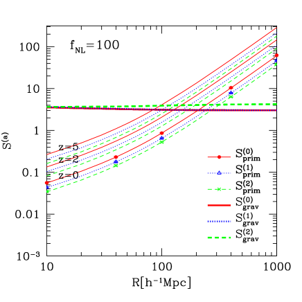
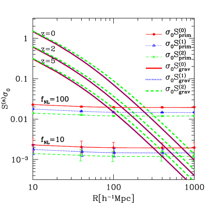
Figure 3: (Left) Skewness parameters, $S^{(a)}(z)$, for $a=0$ (solid), 1 (dotted), and 2 (dashed), at $z=0$, 2, 5. (Right) Skewness parameters multiplied variance, $S^{(a)}(z)\sigma_{0}$, for $a=0$ (solid), 1 (dotted), and 2 (dashed), at $z=0$, 2, 5. In both figures, the thick lines show the skewness parameters from non-linear gravitational clustering, $S_{\rm grav}^{(a)}$ (Eq. [LABEL:eq:sgrav0–48]), while the thin lines show the primordial skewness parameters, $S_{\rm prim}^{(a)}$, with $f_{\rm NL}=100$ (and $10$ in the right panel). The symbols show the skewness parameters measured from numerical simulations of non-Gaussian matter density fluctuations. Note that $S_{\rm grav}^{(a)}$ and $S_{\rm prim}^{(a)}\sigma_{0}$ are independent of $z$.

In order to investigate how important the effect of $B_{\rm grav}$ is, let us define the skewness parameters that are contributed solely by $B_{\rm prim}$ or $B_{\rm grav}$. Substituting $B_{\rm grav}$ and $\sigma_{{\rm m},j}(z)$ for $B_{\rm g}$ and $\sigma_{{\rm g},j}$, respectively, in equation (40), (41), and (42), we obtain $S^{(a)}_{\rm grav}$ ($a=0$, 1, and 2) given by (Matsubara, 2003)

$$S^{(0)}_{\rm grav}(z) = \frac{3}{28\pi^{4}\sigma_{{\rm m},0}^{4}(z)}\left[5I_{220}(z)+7I_{131}(z)+2I_{222}(z)\right],$$

$$S^{(1)}_{\rm grav}(z) = \frac{3}{56\pi^{4}\sigma_{{\rm m},0}^{2}(z)\sigma_{{\rm m},1}^{2}(z)}\left[10I_{240}(z)+12I_{331}(z)\right.$$ (47)

$$\left.+7I_{151}(z)+11I_{242}(z)+2I_{333}(z)\right],$$

$$S^{(2)}_{\rm grav}(z) = \frac{9}{56\pi^{4}\sigma_{{\rm m},1}^{4}(z)}\left[5I_{440}(z)+7I_{351}(z)-3I_{442}(z)\right.$$ (48)

$$\left.-7I_{353}(z)-2I_{444}(z)\right],$$

where

$$I_{mnr}(z) \equiv \int^{\infty}_{0}dk_{1}\int^{\infty}_{0}dk_{2}\int^{1}_{-1}d\mu W(k_{1}R)W(k_{2}R)$$ (49)

$$\times W(k_{12}R)k_{1}^{m}k_{2}^{n}\mu^{r}P_{\rm m}(k_{1},z)P_{\rm m}(k_{2},z).$$

Note that $\sigma_{{\rm g},j}=b_{1}\sigma_{{\rm m},j}$. Similarly, we also calculate the primordial skewness parameters, $S^{(a)}_{\rm prim}$, by substituting $B_{\rm prim}$ and $\sigma_{{\rm m},j}(z)$ for $B_{\rm g}$ and $\sigma_{{\rm g},j}(z)$, respectively, in equation (40), (41), and (42). These skewness parameters are related to the skewness parameters of the total galaxy bispectrum as

$$S_{\rm g}^{(a)}=\frac{S^{(a)}_{\rm prim}+S^{(a)}_{\rm grav}}{b_{1}}+\frac{3b_{2}}{b_{1}^{2}}.$$ (50)

In Figure 3 we compare $S_{\rm prim}^{(a)}(z)$ and $S_{\rm grav}^{(a)}(z)$ at $z=0$, 2, and 5, as a function of a smoothing length, $R$, which is in units of $h^{-1}$ Mpc. (The smoothing kernel $W(kR)$ is set to be a Gaussian filter, $W(kR)=\exp(-k^{2}R^{2}/2)$.) Non-Gaussianity from non-linear gravitational clustering always gives positively skewed density fluctuations, $S^{(a)}_{\rm grav}>0$. Primordial non-Gaussianity with a positive $f_{\rm NL}$ also yields positively skewed density fluctuations; however, primordial non-Gaussianity with a negative $f_{\rm NL}$ yields negatively skewed density fluctuations, which may be distinguished from $S^{(a)}_{\rm grav}$ more easily. As the smoothing scale, $R$, increases (i.e., density fluctuations become more linear), non-Gaussianity from non-linear clustering, $S^{(a)}_{\rm grav}\sigma_{{\rm m},0}$, becomes weaker, while primordial non-Gaussianity, $S^{(a)}_{\rm prim}\sigma_{{\rm m},0}$, remains nearly the same. At $z=0$, the primordial contribution exceeds non-linear gravity only at very large scales, $R>200~{}h^{-1}$ Mpc for $f_{\rm NL}=100$, and $R>800~{}h^{-1}$ Mpc for $f_{\rm NL}=10$. As higher redshift, on the other hand, non-linearity is much weaker and therefore the primordial contribution dominates at relatively smaller spatial scales, $R>120~{}h^{-1}$ Mpc and $80~{}h^{-1}$ Mpc at $z=2$ and 5, respectively, for $f_{\rm NL}=100$. Unlike for the CMB, all the skewness parameters of galaxies exhibit similar dependence on the smoothing scales. The perturbation formula is valid when the amplitude of the second order correction of MFs is small, $S^{(k)}\sigma_{0}\ll 1$, that is, $f_{\rm NL}\ll 5000$.

4.2 Measuring $f_{\rm NL}$ from Minkowski Functionals of LSS

Figure 4 shows the perturbation predictions for the MFs from primordial non-Gaussianity with $f_{\rm NL}=100$, 50, 0, $-50$, and $-100$. For comparison, we also show the MFs computed from numerical simulations with $f_{\rm NL}=100$. In Appendix A.4 we describe our methods for computing MFs from the LSS data. In Appendix A.5 we describe our methods for simulating the LSS data with primordial non-Gaussianity (but without any effects from non-linear gravitational clustering or galaxy bias). The error-bars are estimated from variance among 2000 realizations divided by $\sqrt{2000}$. The left panels show the MFs, while the right panels show the difference between the non-Gaussian and Gaussian MFs, divided by the maximum amplitude of each MF. We find that the analytical perturbation predictions agree with the numerical simulations very well.

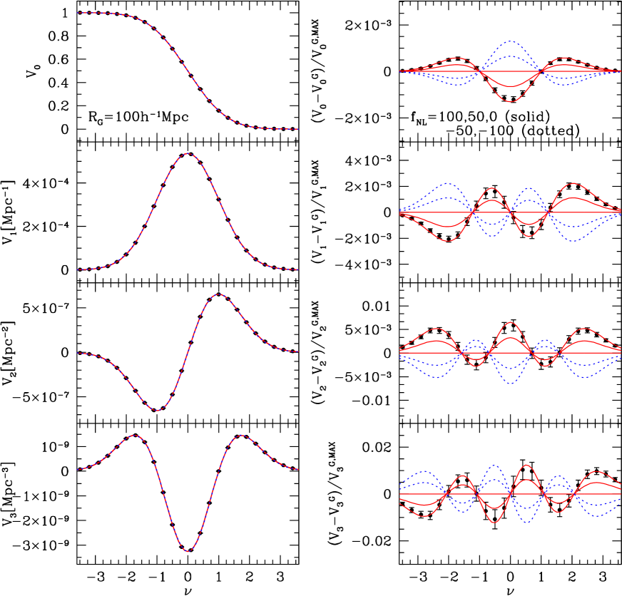
Figure 4: Analytical predictions for the Minkowski Functionals of LSS with primordial non-Gaussianity characterized by $f_{\rm NL}=100$, 50, 0 (solid), $-50$, and $-100$ (dotted), for a Gaussian smoothing length of $R=100~{}h^{-1}$ Mpc. The left panels show the MFs $V_{k}$ ($k=0$, 1, 2, and 3 from top to bottom), while the right panels show the difference between non-Gaussian and Gaussian MFs, $V_{k}^{G}$, divided by the maximum amplitude of $V_{k}^{G}$. The symbols show the average and error of the MFs calculated from 2000 realizations of simulated primordial non-Gaussian density fluctuations with $f_{\rm NL}=100$.

Let us comment on some subtlety that exists in the comparison between the perturbation predictions and numerical simulations. The MFs measured from numerical simulations often deviate from the analytical predictions, even for Gaussian fluctuations, due to subtle pixelization effects. The MFs from our Gaussian simulations deviate from the analytical predictions at the level of $10^{-2}$ when normalized to the maximum amplitude of each MF. It is important to remove this bias, as the magnitude of this effect is comparable to or larger than the effect of primordial non-Gaussianity with $f_{\rm NL}=100$ ($10^{-3}$ for $V_{0}$ and $10^{-2}$ for $V_{3}$). Therefore, it is often necessary to re-calibrate the Gaussian predictions for the pixelization effects by running a large number of Gaussian realizations. However, we have found that the difference between the Gaussian and non-Gaussian MFs measured from simulations does agree with the perturbation predictions without any corrections. Therefore, one may use the following procedure for calculating the correct non-Gaussian MFs:

• Use the analytical formulae (Eq. [2]) to calculate the difference between the Gaussian and non-Gaussian MFs,

  $$\Delta V_{k}^{(d)}(\nu,f_{\rm NL})\equiv V_{k}^{(d)}(\nu,f_{\rm NL})-V_{k}^{(d)}(\nu,f_{\rm NL}=0).$$ (51)

• Run Gaussian simulations. Estimate the average MFs from these Gaussian simulations, $\tilde{V}_{k}^{(d)}(\nu,f_{\rm NL}=0)$. This would be slightly different from the analytical formula, $V_{k}^{(d)}(\nu,f_{\rm NL}=0)$, due to the pixelization and boundary effects. Note that the same simulations may be used to obtain the covariance matrix of MFs.

• Calculate the final non-Gaussian predictions as

  $$\tilde{V}_{k}^{(d)}(\nu,f_{\rm NL})=\tilde{V}_{k}^{(d)}(\nu,f_{\rm NL}=0)+\Delta V_{k}^{(d)}(\nu,f_{\rm NL}).$$ (52)

We estimate the projected errors on $f_{\rm NL}$ from LSS using the Fisher information matrix in the same way as CMB (see § 3.2). We compute the covariance matrix of MFs from 2000 realizations of Gaussian density fluctuations in a 1 Gpc³ cubic box. For simplicity, we focus on the large scales and ignore non-Gaussianity from non-linear gravitational evolution. (The minimum smoothing scale is $R=60~{}h^{-1}$ Mpc). We also ignore shot noise.

Table 4 shows the projected 1-$\sigma$ errors on $f_{\rm NL}$ from a galaxy survey covering 1 $h^{-3}~{}{\rm Gpc}^{3}$ volume. This volume would correspond to e.g., a galaxy survey covering 300 deg² on the sky at $5.5<z<6.5$. Note that these constraints are independent of $z$ when non-linear gravitational evolution is ignored, as $S_{\rm prim}^{(a)}\sigma_{0}$ is independent of $z$. We have assumed a linear galaxy bias ($b_{2}=0$) in the second column, while we have marginalized $b_{2}/b_{1}$ in the third column. A more realistic prediction would lie between these two cases, as we can use the power spectrum and bispectrum to put some constraints on $b_{2}$. We find better constraints from smaller smoothing scales for a given survey volume, simply because we have more modes on smaller scales. The limits on $f_{\rm NL}$ from a 1 $h^{-3}~{}{\rm Gpc}^{3}$ survey are not very promising, $|f_{\rm NL}|\sim 270$ at the 68% confidence level; thus, one would need the survey volume as large as 25 $h^{-3}~{}{\rm Gpc}^{3}$ to make the LSS constraints comparable to the WMAP constraints (using the MFs only). This could be done by a survey covering $\sim 2000$ deg² at $3.5<z<6.5$. One would obviously need more volume to make it comparable to the Planck data.

Table 4: Constraints on $f_{\rm NL}$ from the MFs of LSS in a galaxy survey covering 1 $h^{-3}~{}{\rm Gpc}^{3}$ volume. All of the four MFs have been combined. The first column shows the smoothing scales that have been used. The second column shows the constraints assuming a linear bias ($b_{2}=0$), while the third column shows the constraints with $b_{2}/b_{1}$ marginalized. Note that these constraints are independent of $z$ when non-linear gravitational evolution is ignored, as $S_{\rm prim}^{(a)}\sigma_{0}$ is independent of $z$.

$R~{}h^{-1}$ Mpc	$f_{\rm NL}$ ($b_{2}/b_{1}=0$)	$f_{\rm NL}$ ($b_{2}/b_{1}$ marginalized)
$100,120~{}\&~{}140$	$540$	$1200$
$80,100~{}\&~{}120$	$350$	$670$
$60,80~{}\&~{}100$	$270$	$630$

5 Summary and Conclusions

We have derived analytical formulae of the MFs for CMB and LSS using a perturbation approach. The analytical formula is useful for studying the behavior of MFs and estimating the observational constraints on $f_{\rm NL}$ without relying on non-Gaussian numerical simulations. The perturbation approach works when the skewness parameters multiplied by variance, $S^{a}\sigma_{0}$, is much smaller than unity, i.e., $|f_{\rm NL}|\ll 3300$ for CMB and $|f_{\rm NL}|\ll 5000$ for LSS, both of which are satisfied by the current observational constraints from WMAP (Komatsu et al., 2003; Creminelli et al., 2006; Spergel et al., 2006). We have shown that the perturbation predictions agree with non-Gaussian numerical realizations very well.

We have used the Fisher matrix analysis to estimate the projected constraints on $f_{\rm NL}$ expected from the observations of CMB and LSS. We have found that the projected 1-$\sigma$ error on $f_{\rm NL}$ from the WMAP should reach 50, which is consistent with the MF analysis given in Komatsu et al. (2003); Spergel et al. (2006), and is comparable to the current constraints from the bispectrum analysis given in Komatsu et al. (2003); Creminelli et al. (2006); Spergel et al. (2006). The MFs from the WMAP 8-year and Planck observations should be sensitive to $|f_{\rm NL}|\sim 40$ and 20, respectively, at the 68% confidence level.

As the MFs are solely determined by the weighted sum of the bispectrum for $|f_{\rm NL}|\ll 3300$ for CMB and $|f_{\rm NL}|\ll 5000$ for LSS, the MFs do not contain information more than the bispectrum. However, this does not imply that the MFs are useless for measuring primordial non-Gaussianity by any means. The important distinction between the MFs and bispectrum is that the MFs are intrinsically defined in real space, while the bispectrum is defined in Fourier space. The systematics in the data are most easily dealt with in real space, and thus the MFs should be quite useful in this regard. Therefore, in the presence of real-world issues such as inhomogeneous noise, foreground, masks, etc., these two approaches should be used to check for consistency of the results.

In this paper we have calculated the MFs from primordial non-Gaussianity with a scale-independent $f_{\rm NL}$. It is easy to extend our calculations to a scale-dependent $f_{\rm NL}$. All one needs to do is to calculate the form of the bispectrum with a scale-dependent $f_{\rm NL}$ (e.g., Babich et al., 2004; Liguori et al., 2006), and use it to obtain the skewness parameters, $S^{(a)}$ (Eqs. [20–22] for CMB and Eqs. [40–42] for LSS). The MFs are then given by equation (2) in terms of the skewness parameters. Also, we have not included non-Gaussianity from secondary anisotropy such as the Sunyaev-Zel’dovich effect, Rees-Sciama effect, patchy reionization, weak lensing effect, extragalactic radio sources, etc. It is again straightforward to calculate the MFs from these sources using our formalism, as long as the form of the bispectrum is known (e.g., Spergel & Goldberg, 1999; Goldberg & Spergel, 1999; Cooray & Hu, 2000; Komatsu & Spergel, 2001; Verde & Spergel, 2002).

The constraints on primordial non-Gaussianity from the MFs of LSS in a galaxy survey covering 1 $h^{-3}~{}{\rm Gpc}^{3}$ volume are about 5 times weaker than those from the MFs of CMB in the WMAP data. One would therefore need the survey volume as large as 25 $h^{-3}~{}{\rm Gpc}^{3}$ to make the LSS constraints comparable to the WMAP constraints (using the MFs only). This could be done by a survey covering $\sim 2000$ deg² at $3.5<z<6.5$. One would obviously need more volume to make it comparable to the Planck data. The MFs from LSS are less sensitive to primordial non-Gaussianity because non-Gaussianity from the non-linear evolution of gravitational clustering exceeds the primordial contribution at $R<200$, $120$, and 80 $h^{-1}$ Mpc at $z=0$, 2, and 5, respectively, which severely limits the amount of LSS data available to constrain primordial non-Gaussianity.

Appendix A Measuring Minkowski Functionals from CMB and LSS

In this Appendix we describe our methods for computing the MFs from the CMB and LSS data. We also describe our simulations of CMB and LSS.

A.1 Computational Method: CMB

We estimate the MFs from pixelized CMB sky maps by integrating a combination of first and second angular derivatives of temperature anisotropy, ${\cal I}_{k}$, over the sky (Schmalzing & G$\acute{\rm o}$rski, 1998),

$$V_{k}^{(2)}(\nu)=\frac{\sum_{i=1}^{n_{\rm pix}}w_{i}{\cal I}_{k}({\mathbf{\Omega}}_{i})}{\sum_{i=1}^{n_{\rm pix}}w_{i}},$$ (A1)

where ${\mathbf{\Omega}}_{i}$ is the unit vector pointing toward a given position on the sky. We set the weight of $i-$th pixel, $w_{i}$, to be 1 when the pixel at ${\mathbf{\Omega}}_{i}$ is outside of the survey mask, and 0 otherwise. We calculate ${\cal I}_{k}$ at ${\mathbf{\Omega}}_{i}$ from covariant derivatives of temperature anisotropy divided by its standard deviation, $u({\mathbf{\Omega}}_{i})\equiv(\Delta T/T)/\sigma_{0}$,

$${\cal I}_{0} = \Theta(u-\nu),$$ (A2)

$${\cal I}_{1} = \frac{1}{4}F(u-\nu)\sqrt{u^{2}_{;\theta}+u^{2}_{;\phi}},$$ (A3)

$${\cal I}_{2} = \frac{1}{2\pi}F(u-\nu)\frac{2u_{;\theta}u_{;\phi}u_{;\theta\phi}-u^{2}_{;\theta}u_{;\phi\phi}-u^{2}_{;\phi}u_{;\theta\theta}}{u^{2}_{;\theta}+u^{2}_{;\phi}}.$$ (A4)

The function $F(u-\nu)$ has a value of $1/\Delta\nu$ ($\Delta\nu$ is the binning width of $\nu$) when $u$ is within $[\nu-\Delta\nu/2,\nu+\Delta\nu/2]$, and 0 otherwise. Covariant derivatives are related to the partial derivatives as

$$u_{;\theta} = u_{,\theta},$$ (A5)

$$u_{;\phi} = \frac{1}{\sin\theta}u_{,\phi},$$ (A6)

$$u_{;\theta\theta} = u_{,\theta\theta},$$ (A7)

$$u_{;\theta\phi} = \frac{1}{\sin\theta}u_{,\theta\phi}-\frac{\cos\theta}{\sin^{2}\theta}u_{,\phi},$$ (A8)

$$u_{;\phi\phi} = \frac{1}{\sin^{2}\theta}u_{,\phi\phi}+\frac{\cos\theta}{\sin\theta}u_{,\theta}.$$ (A9)

The first derivative of the temperature field $u_{,i}(i=\theta,$ or $\phi)$ are calculated in Fourier space as;

$$u_{,i} = \sum_{lm}a_{lm}Y_{lm,i}$$ (A10)

$$Y_{lm,\theta} = \left\{\begin{array}[]{lc}\displaystyle\frac{l}{\tan\theta}Y_{lm}-\sqrt{\frac{2l+1}{2l-1}(l^{2}-m^{2})}\frac{1}{\sin\theta}Y_{l-1m}&(|m|<l)\\ \displaystyle\frac{l}{\tan\theta}Y_{lm}&(m=l)\end{array}\right.$$ (A13)

$$Y_{lm,\phi} = imY_{lm}$$ (A14)

The second derivatives are also computed as

$$u_{,ij} = \sum_{lm}a_{lm}Y_{lm,ij}$$ (A16)

$$Y_{lm,\theta\theta} = \left[-\left(l(l+1)-\frac{m^{2}}{\sin^{2}\theta}\right)Y_{lm}-\frac{1}{\tan\theta}Y_{lm,\theta}\right]$$ (A17)

$$Y_{lm,\theta\phi} = imY_{lm,\theta}$$ (A18)

$$Y_{lm,\phi\phi} = -m^{2}Y_{lm}$$ (A19)

We calculate the MFs of temperature anisotropy for $\nu$ from $-3$ to $3$ with $\Delta_{\nu}=0.24$, which yields $25$ bins per each MF.

A.2 Simulating WMAP Data

In order to quantify uncertainties in the estimated MFs from cosmic variance and various effects, we simulate Gaussian temperature anisotropy maps with noise characteristics of the WMAP data. We generate 1000 Gaussian realizations of CMB temperature anisotropy using the HEALPix package (G$\acute{\rm o}$rski et al., 2005). We use $N_{\rm side}=128$, $256$ and $512$ for $\theta_{s}\geq 40$, $40>\theta_{s}\geq 10$, $10>\theta_{s}$ respectively. The number of pixels is given by $n_{\rm pix}=12N_{\rm side}^{2}$. From each sky realization we construct eight simulated maps of WMAP differential assemblies (DAs), Q1, Q2, V1, V2, W1, W2, W3, and W4, by convolving the sky map with the beam transfer function in each DA (Page et al., 2003a), and adding independent Gaussian noise realizations following the noise pattern in each DA. Each pixel is given noise variance of $\sigma_{0,{\rm noise}}^{2}/N_{\rm obs}({\mathbf{\Omega}}_{i})$, where $N_{\rm obs}({\mathbf{\Omega}}_{i})$ is the number of observations per pixel, and $\sigma_{0,{\rm noise}}$ is given in Bennett et al. (2003a). We then co-add the eight maps by weighting each map by $\bar{N}_{\rm obs}/\sigma_{0,{\rm noise}}^{2}$, where $\bar{N}_{\rm obs}$ is the full-sky average of $N_{\rm obs}({\mathbf{\Omega}}_{i})$. Finally, we mask the co-added map by the $Kp0$ Galaxy mask (including point-source mask) provided by Bennett et al. (2003b). This mask leaves $76.8$% of the sky available for the subsequent data analysis. In addition to WMAP one-year data, we also simulate the future WMAP eight-year data, by simply multiplying $N_{\rm obs}$ by a factor of $8$.

Before we estimate the MFs from each simulated map, we smooth it using a Gaussian filter with a smoothing scale of $\theta_{s}$,

$$W_{l}=\exp\left[-\frac{1}{2}l(l+1)\theta_{s}^{2}\right].$$ (A20)

To remove the effect of survey mask, we calculate the Minkowski Functionals by limiting the pixels where the five measurements, $\sigma,\sigma_{1},$ and $S^{(k)}(k=0,1,\&2)$, have nearly equal values between the field with survey mask and that without survey mask. We use the pixels where the difference is within $5\%$ of each standard deviation for $\theta_{s}=20$ and $40$ arcmin and $10\%$ for $\theta_{s}=70$ and $100$ arcmin. For $\theta_{s}=5$ and $10$ arcmin, we use the pixels as long as they are away from the boundary of the mask by more than $2\theta_{s}$. Table 5 lists the sky fraction used in the analysis for each smoothing scale.

Table 5: Sky fraction used for the calculation of MFs

$\theta_{s}$	sky fraction [%]
$100$	$13$
$70$	$26$
$40$	$41$
$20$	$62$
$10$	$73$
$5$	$75$

The mean density over the pixels which are used for the calculation of MFs is not completely zero and thus we subtract it from the density field to satisfy zero mean in each realization.

A.3 Simulating Planck Data

For the simulations of the Planck data, we follow the same procedure as the WMAP simulations. Each realization is a coadded map of 9 bands with the inverse weight of the noise variance listed in Table 6. We approximate the beam transfer function as a Gaussian function, $\exp(-\theta_{\rm beam}^{2}l(l+1)/2)$, where $\theta_{\rm beam}=\theta_{\rm FWHM}/\sqrt{8\ln(2)}$. We add the homogeneous noise distribution with the noise variance per pixel $\sigma_{\rm noise}^{2}$ given by

$$\frac{1}{\sigma_{\rm noise}^{2}}=\sum_{i}\left(\frac{T}{\Delta T}\right)^{(i)2}\frac{4\pi/n_{\rm pix}}{(\theta_{\rm FWHM}^{(i)})^{2}},$$ (A21)

where $i$ denotes each band, and $n_{\rm pix}=12N_{\rm side}^{2}$ is the number of pixels in simulated maps. We use the $Kp0$ mask to define the survey area for the Planck simulations, in exactly the same manner as for the WMAP simulations.

Table 6: Approximate instrument specifications of the Planck satellite (http://www.rssd.esa.int/Planck). The central frequency, full width at half maximum (FWHM) of beam size, $\theta_{\rm FWHM}$, and noise per pixel ($\Delta T/T$ per $\theta_{\rm FWHM}^{2}$) for 14 months of observations are shown per each frequency channel.

Instrument	LFI				HFI
Center Frequency [GHz]	$30$	$44$	$70$		$100$	$143$	$217$	$353$	$545$	$857$
Beam size $\theta_{\rm FWHM}$ [arcmin]	$33$	$24$	$14$		$9.5$	$7.1$	$5$	$5$	$5$	$5$
Pixel Noise $\Delta T/T$ [$10^{6}$]	$2$	$2.7$	$4.7$		$2.5$	$2.2$	$4.8$	$14.7$	$147$	$6700$

A.4 Computational Method: LSS

We use two complementary routines to compute the MFs of a density field on the grids. The first approach is often called Koenderink invariants (Koenderink, 1984) in which the surface integrals of the curvature are transformed into the volume integral of invariants formed from the first and second derivatives of the density fluctuations. The second method, which is called Crofton’s formula (Crofton, 1868; Schmalzing & Buchert, 1997; Koenderink, 1984), is based on the integral geometry and the calculation reduce to simply counting the elementary cells (e.g., cubes, squares, lines, and points for the cubic meshes). The outline of these methods are summarized in Schmalzing & Buchert (1997) and the observational application to SDSS galaxy samples are performed by Hikage et al. (2003).

A.5 Simulating LSS Data with Primordial Non-Gaussianity

We calculate the MFs of density field in a cubic box with a length of $1~{}h^{-1}$ Gpc, but ignore the observational effects such as survey geometry, for simplicity. We also ignore non-linear gravitational clustering or galaxy bias in order to isolate the effect from primordial non-Gaussianity. (The purpose of this simulation is to check the accuracy of our perturbation predictions for the form of MFs from primordial non-Gaussianity.) To simulate the LSS data with primordial non-Gaussianity, we first generate a Gaussian potential field in a cubic box with a length of $1~{}h^{-1}$ Gpc, assuming that the power spectrum of potential is $P_{\phi}(k)\propto k^{n_{s}-4}$ where $n_{s}=0.967$. We inversely Fourier-transform it into real space to obtain $\phi({\mathbf{x}})$. (The number of grids is $128^{3}$.) We then construct a non-Gaussian potential field, $\Phi({\mathbf{x}})$, using equation (eq.[1]) for a given $f_{\rm NL}$. We finally convert it to the matter density field by multiplying $\Phi$ by $M(k)$ in Fourier space (see Eq. [B10]). We have generated 2,000 realizations of the non-Gaussian density field.

Appendix B Derivation of Galaxy Bispectrum

In this Appendix we derive the perturbative formula for the galaxy bispectrum including primordial non-Gaussianity, non-linearity in gravitational clustering, and non-linearity in galaxy biasing, in the weakly non-linear regime (Verde et al., 2000; Scoccimarro et al., 2004). In the weakly non-linear regime, it would be reasonable to assume that the galaxy biasing is local and deterministic. We then expand the galaxy density contrast, $\delta_{\rm g}$, perturbatively in terms of the underlying matter density contrast, $\delta_{\rm m}$, as (Fry & Gaztan$\tilde{\rm a}$ga, 1993)

$$\delta_{\rm g}(z)=b_{0}(z)+b_{1}(z)\delta_{\rm m}(z)+\frac{b_{2}(z)}{2}\delta_{\rm m}^{2}(z)+{\cal O}(\delta_{\rm m}^{3}).$$ (B1)

where $b_{0}(z)$ is determined such that $\langle\delta_{\rm g}(z)\rangle=0$. Here, $b_{1}(z)$ and $b_{2}(z)$ are the time-dependent galaxy bias parameters. The power spectrum and bispectrum of the galaxy distribution, $P_{\rm g}$ and $B_{\rm g}$, respectively, are then given by those of the underlying matter distribution as

$$P_{\rm g}(k,z) = b_{1}^{2}(z)P_{\rm m}(k,z),$$ (B2)

$$B_{\rm g}(k_{1},k_{2},k_{3},z) = b_{1}^{3}(z)B_{\rm m}(k_{1},k_{2},k_{3},z)+b_{1}^{2}(z)b_{2}(z)[P_{\rm m}(k_{1},z)P_{\rm m}(k_{2},z)+(\mbox{cyc.})],$$ (B3)

respectively. If the underlying mass distribution obeyed Gaussian statistics, its bispectrum would vanish exactly, $B_{\rm m}\equiv 0$; however, the non-linear evolution of density fluctuations due to gravitational instability makes $\delta_{\rm m}$ slightly non-Gaussian in the weakly non-Gaussian regime, yielding non-zero bispectrum.

The second-order correction to the density fluctuations from non-linear gravitational clustering gives the following equation,

$$\tilde{\delta}_{{\rm m},{\mathbf{k}}}(z)=\tilde{\delta}_{{\rm L},{\mathbf{k}}}(z)+\int d^{3}qF_{2}({\mathbf{q}},{\mathbf{k}}-{\mathbf{q}})\tilde{\delta}_{{\rm L},{\mathbf{q}}}(z)\tilde{\delta}_{{\rm L},{\mathbf{k}}-{\mathbf{q}}}(z),$$ (B4)

where $\tilde{\delta}_{{\rm L},{\mathbf{k}}}(z)$ is the linear (but non-Gaussian) density fluctuations, and

$$F_{2}({\mathbf{k}}_{1},{\mathbf{k}}_{2})=\frac{5}{7}+\frac{{\mathbf{k}}_{1}\cdot{\mathbf{k}}_{2}}{2k_{1}k_{2}}\left(\frac{k_{1}}{k_{2}}+\frac{k_{2}}{k_{1}}\right)+\frac{2}{7}\frac{({\mathbf{k}}_{1}\cdot{\mathbf{k}}_{2})^{2}}{k_{1}^{2}k_{2}^{2}},$$ (B5)

is the time-independent kernel describing mode-coupling due to non-linear clustering of matter density fluctuations in the weakly non-linear regime. Equation (B5) is exact only in an Einstein-de Sitter universe, but the corrections in other cosmological models are small (e.g., Bernardeau, 1994). The power spectrum and bispectrum of the underlying mass density distribution, $P_{\rm m}$ and $B_{\rm m}$, are thus given in terms of the linear and non-linear contributions:

$$P_{\rm m}(k,z) = P_{\rm L}(k,z),$$ (B6)

$$B_{\rm m}(k_{1},k_{2},k_{3},z) = B_{\rm prim}(k_{1},k_{2},k_{3},z)+2\left[F_{2}({\mathbf{k}}_{1},{\mathbf{k}}_{2})P_{\rm L}(k_{1},z)P_{\rm L}(k_{2},z)+(\mbox{cyc.})\right].$$ (B7)

Note that we have ignored the non-linear contributions in the power spectrum. That is to say, the power spectrum is still described by linear perturbation theory.

The remaining task is to relate $\delta_{\rm L}(z)$ to Bardeen’s curvature perturbations during the matter era, $\Phi$. One may use Poisson’s equation for doing this:

$$k^{2}\tilde{\Phi}_{\mathbf{k}}T(k)=4\pi G\rho_{\rm m}(z)\frac{\tilde{\delta}_{{\rm m},{\mathbf{k}}}(z)}{(1+z)^{2}}=\frac{3}{2}\Omega_{\rm m}H_{0}^{2}\tilde{\delta}_{{\rm m},{\mathbf{k}}}(z)(1+z),$$ (B8)

where $T(k)$ is the linear transfer function that describes the evolution of density fluctuations during the radiation era and the interactions between photons and baryons (Eisenstein & Hu, 1999). Note that $\Phi$ is independent of time during the matter era. At very early times, say, $z=z_{*}\sim 10^{3}$, the non-linear evolution may be safely ignored at the scales of interest, and one obtains

$$\tilde{\delta}_{{\rm L},{\mathbf{k}}}(z_{*})=\frac{M(k)\tilde{\Phi}_{\mathbf{k}}}{1+z_{*}},$$ (B9)

where

$$M(k)\equiv\frac{2}{3}\frac{k^{2}T(k)}{\Omega_{\rm m}H_{0}^{2}}.$$ (B10)

Therefore, using the quadratic non-Gaussian model given in equation (1), one obtains the linear power spectrum at $z=z_{*}$,

$$P_{\rm L}(k,z_{*})=\frac{M^{2}(k)}{(1+z_{*})^{2}}P_{\phi}(k),$$ (B11)

and the primordial bispectrum at $z=z_{*}$,

$$B_{\rm prim}(k_{1},k_{2},k_{3},z_{*}) = 2f_{\rm NL}\frac{M(k_{1})M(k_{2})M(k_{3})}{(1+z_{*})^{3}}[P_{\phi}(k_{1})P_{\phi}(k_{2})+(\mbox{cyc.})]$$ (B12)

$$= 2f_{\rm NL}(1+z_{*})\left[\frac{P_{\rm L}(k_{1},z_{*})P_{\rm L}(k_{2},z_{*})M(k_{3})}{M(k_{1})M(k_{2})}+(\mbox{cyc.})\right],$$

where $P_{\phi}(k)\propto k^{n_{s}-4}$ is the power spectrum of $\phi$ and we have ignored the higher-order terms. We then use the linear growth rate of density fluctuations, $\delta_{\rm L}\propto D(z)$, to evolve the linear bispectrum forward in time:

$$B_{\rm prim}(k_{1},k_{2},k_{3},z)=2f_{\rm NL}\frac{(1+z_{*})D(z_{*})}{D(z)}\left[\frac{P_{\rm L}(k_{1},z)P_{\rm L}(k_{2},z)M(k_{3})}{M(k_{1})M(k_{2})}+(\mbox{cyc.})\right].$$ (B13)

One may simplify this expression by normalizing the growth rate such that

$$D(z_{*})=\frac{1}{1+z_{*}}.$$ (B14)

Note that this condition gives the normalization of $D(z)$ that is actually independent of the choice of $z_{*}$, when $z_{*}$ is taken to be during the matter era.

By putting all the terms together, we finally obtain the following form of $B_{\rm g}(k_{1},k_{2},k_{3},z)$:

$$B_{\rm g}(k_{1},k_{2},k_{3},z) = 2f_{\rm NL}\frac{b_{1}^{3}(z)}{D(z)}\left[\frac{P_{\rm m}(k_{1},z)P_{\rm m}(k_{2},z)M(k_{3})}{M(k_{1})M(k_{2})}+(\mbox{cyc.})\right]$$ (B15)

$$+2b_{1}^{3}(z)\left[F_{2}({\mathbf{k}}_{1},{\mathbf{k}}_{2})P_{\rm m}(k_{1},z)P_{\rm m}(k_{2},z)+(\mbox{cyc.})\right]$$

$$+b_{1}^{2}(z)b_{2}(z)[P_{\rm m}(k_{1},z)P_{\rm m}(k_{2},z)+(\mbox{cyc.})].$$

We use this formula to calculate the skewness parameters that are used for the MFs of the galaxy distribution.

While the perturbative formula for the MFs derived by Matsubara (2003) (See § 2) works well for $\Phi$, it is not immediately clear if it works for $\delta_{\rm g}$ because of the $k$-dependent coefficient, $\tilde{\delta}_{{\rm g},{\mathbf{k}}}\propto M(k)\tilde{\Phi}_{\mathbf{k}}$. In Appendix D we show that the perturbative formula still works, as long as $f_{\rm NL}$ is not very large. The current observational constraints on $f_{\rm NL}$ already guarantee that the perturbative formula for the MFs of the galaxy distribution provides an excellent approximation.

Appendix C MFs of CMB: Analytical Formula vs Simulations in the Sachs–Wolfe Limit

We compare the perturbative formula of MFs for CMB with Monte-Carlo realizations of non-Gaussian temperature anisotropy in the Sachs-Wolfe regime, in order to check the accuracy of our formalism.

The angular power spectrum spectrum is set to be $l(l+1)C_{l}^{\rm SW}/2\pi=10^{-10}$. In the Sachs-Wolfe limit, $\Delta T^{\rm SW}/T=-\Phi/3$, the non-Gaussian maps of CMB temperature anisotropy may be constructed from the Gaussian maps, $\Delta T_{G}/T$, by the following simple mapping:

$$\frac{\Delta T^{\rm SW}}{T}=\frac{\Delta T_{G}}{T}-3f_{\rm NL}\left[\left(\frac{\Delta T_{G}}{T}\right)^{2}-\left\langle\left(\frac{\Delta T_{G}}{T}\right)^{2}\right\rangle\right].$$ (C1)

We calculate the MFs from 6000 realizations of the non-Gaussian CMB maps and compare them with the perturbation predictions (Eq.[2]). The skewness parameters can be calculated from the reduced bispectrum of CMB in the Sachs-Wolfe limit,

$$b_{l_{1}l_{2}l_{3}}=-6f_{\rm NL}(C_{l_{1}}^{\rm SW}C_{l_{2}}^{\rm SW}+C_{l_{2}}^{\rm SW}C_{l_{3}}^{\rm SW}+C_{l_{3}}^{\rm SW}C_{l_{1}}^{\rm SW}).$$ (C2)

Figure 5 shows that the MFs from Monte-Carlo realizations agree with the perturbation predictions very well. The comparison with the full simulations that include the full radiation transfer function will be reported elsewhere. (For subtlety in this comparison arising from pixelization and boundary effects, see § 4.2.)

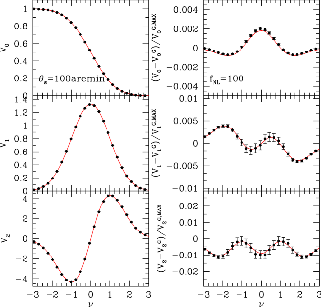
Figure 5: Comparison between the MFs calculated from the analytical perturbation predictions (solid lines) and the numerical simulations (symbols) in the Sachs-Wolfe limit. We have used $\theta_{s}=100$ arcmin and $f_{\rm NL}=100$.

Appendix D Validity of Perturbative Formulae for $N-$th order corrections of Primordial Non-Gaussianity

We consider the primordial non-Gaussianity extended to $n-$th order corrections of a primordial potential field;

$$\Phi=\epsilon\phi_{0}+\frac{\epsilon^{2}f_{\rm NL}^{(1)}}{2!}(\phi_{0}^{2}-\langle\phi_{0}^{2}\rangle)+\frac{\epsilon^{3}f_{\rm NL}^{(2)}}{3!}\phi_{0}^{3}+\frac{\epsilon^{4}f_{\rm NL}^{(3)}}{4!}(\phi_{0}^{4}-\langle\phi_{0}^{4}\rangle)+\cdot\cdot\cdot+\frac{\epsilon^{n}f_{\rm NL}^{(n-1)}}{n!}(\phi_{0}^{n}-\langle\phi_{0}^{n}\rangle)+\cdot\cdot\cdot,$$ (D1)

where $\epsilon\phi_{0}$ is an auxiliary random-Gaussian field and $f_{\rm NL}^{(n)}$ represents the coefficients of $n$-th order of $\phi$. For convenience, we separate the random-Gaussian field into two parts; the $\epsilon$ represents the amplitude of the primordial potential power spectrum which has the order of $10^{-4}$ and thereby the fluctuation of $\phi_{0}$ is the order unity. The parameter $f_{\rm NL}$ in the equation (1) corresponds to $f_{\rm NL}^{(1)}/2$.

The Fourier transform of $\Phi$ is written by

$$\tilde{\Phi}=\epsilon\tilde{\phi}_{0}+\frac{\epsilon^{2}f_{\rm NL}^{(1)}}{2!}\tilde{\Phi}_{0}^{(2)}+\cdot\cdot\cdot+\frac{\epsilon^{n}f_{\rm NL}^{(n-1)}}{n!}\tilde{\Phi}_{0}^{(n)}+\cdot\cdot\cdot$$ (D2)

where $\tilde{\Phi}_{0}^{(n)}({\mathbf{k}})$ is the Fourier transform of the $n$-th order term, $\phi_{0}^{n}-\langle\phi_{0}^{n}\rangle$, given by

$$\tilde{\Phi}_{0}^{(n)}({\mathbf{k}})=\frac{1}{(2\pi)^{3n-3}}\int d{\mathbf{k}}_{1}\cdot\cdot\cdot\int d{\mathbf{k}}_{n-1}\tilde{\phi}_{0}^{\ast}({\mathbf{k}}_{1})\cdot\cdot\cdot\tilde{\phi}_{0}^{\ast}({\mathbf{k}}_{n-1})\tilde{\phi}_{0}({\mathbf{k}}+{\mathbf{k}}_{1}+\cdot\cdot\cdot{\mathbf{k}}_{n-1})-(2\pi)^{3}\delta_{D}({\mathbf{k}})\langle\phi_{0}^{n}\rangle$$ (D3)

The polyspectra of $\Phi$, $P^{(n)}_{\Phi}$ $(n\geq 2)$, are defined by

$$\langle\Phi({\mathbf{k}}_{1})\cdot\cdot\cdot\Phi({\mathbf{k}}_{n})\rangle_{c}\equiv(2\pi)^{3}\delta_{D}({\mathbf{k}}_{1}+\cdot\cdot\cdot{\mathbf{k}}_{n})P_{\Phi}^{(n)}({\mathbf{k}}_{1},\cdot\cdot\cdot,{\mathbf{k}}_{n})$$ (D4)

where $P^{(2)}_{\Phi}$ and $P^{(3)}_{\Phi}$ correspond to the power spectrum and the bispectrum of $\Phi$ respectively.

According to the diagrammatic method by Matsubara (1995), the lowest order terms of $\epsilon$ for the connected part of $n$-th order moment, called cumulants, are the $n-1$ products of the quadratic moment as follows;

$$P_{\Phi}^{(2)} = \epsilon^{2}P_{\phi_{0}}$$ (D5)

$$P_{\Phi}^{(3)} = \epsilon^{4}f_{\rm NL}^{(1)}(P_{\phi_{0}}(k_{1})P_{\phi_{0}}(k_{2})+(\mbox{cyc.}))$$ (D6)

$$P_{\Phi}^{(4)} = \epsilon^{6}f_{\rm NL}^{(1)2}(P_{\phi_{0}}(k_{1})P_{\phi_{0}}(k_{2})P_{\phi_{0}}(|{\mathbf{k}}_{1}+{\mathbf{k}}_{3}|)+(\mbox{sym.})(12))$$ (D7)

$$+ \epsilon^{6}f_{\rm NL}^{(2)}(P_{\phi_{0}}(k_{1})P_{\phi_{0}}(k_{2})P_{\phi_{0}}(k_{3})+(\mbox{cyc.}))$$

$$P_{\Phi}^{(5)} = \epsilon^{8}f_{\rm NL}^{(1)3}(P_{\phi_{0}}(k_{1})P_{\phi_{0}}(k_{2})P_{\phi_{0}}(|{\mathbf{k}}_{1}+{\mathbf{k}}_{3}|)P_{\phi_{0}}(|{\mathbf{k}}_{2}+{\mathbf{k}}_{4}|)+(\mbox{sym.})(60))$$

$$+ \epsilon^{8}f_{\rm NL}^{(1)}f_{\rm NL}^{(2)}(P_{\phi_{0}}(k_{1})P_{\phi_{0}}(k_{2})P_{\phi_{0}}(k_{3})P_{\phi_{0}}(|{\mathbf{k}}_{1}+{\mathbf{k}}_{4}|)+(\mbox{sym.})(60))$$

$$+ \epsilon^{8}f_{\rm NL}^{(3)}(P_{\phi_{0}}(k_{1})P_{\phi_{0}}(k_{2})P_{\phi_{0}}(k_{3})P_{\phi_{0}}(k_{4})+(\mbox{cyc.}))$$

$$\cdot\cdot\cdot$$

$$P_{\Phi}^{(n)} = \epsilon^{2n-2}\sum^{d_{1}+2d_{2}+\cdot\cdot\cdot nd_{n}=n-2}_{d_{1},d_{2},...,d_{n}}\left(\prod_{m=1,...,n}f_{\rm NL}^{(m)~{}d_{m}}\right)\left[\prod_{k_{AB}(d_{1},d_{2},...,d_{n})}^{n-1}P_{\phi_{0}}(|{\mathbf{k}}_{A}+{\mathbf{k}}_{B}|)+(\mbox{sym.})\right]$$ (D9)

where (sym.)($n$) means the addition of $n$ terms with the subscripts symmetric to the previous term and the edge $(AB)$ is one of the edges in a tree graph $(d_{1},d_{2},...,d_{n})$ which satisfies the condition that $d_{1}+2d_{2}+\cdot\cdot\cdot+nd_{n}=n-2$.

We obtain the $n-$th polyspectrum of $\tilde{\delta}_{\rm L,{\mathbf{k}}}$, $P^{(n)}_{\rm L}$, by

$$P^{(n)}_{\rm L}({\mathbf{k}}_{1},\cdot\cdot\cdot,{\mathbf{k}}_{n-1})=M(k_{1})M(k_{2})\cdot\cdot\cdot M(k_{n})P^{(n)}_{\Phi}.$$ (D10)

The $n$-th order terms of the perturbative formula (eq.[1]) are represented by

$$\frac{\langle\delta_{\rm L}^{n}\rangle_{c}}{\langle\delta_{\rm L}^{2}\rangle^{n/2}},~{}\frac{\langle\delta_{\rm L}^{n-1}\nabla^{2}\delta_{\rm L}\rangle_{c}}{\langle\delta_{\rm L}^{2}\rangle^{n/2-1}\langle(\nabla\delta_{\rm L})\cdot(\nabla\delta_{\rm L})\rangle},~{}\frac{\langle\delta_{\rm L}^{n-3}(\nabla\delta_{\rm L}\cdot\nabla\delta_{\rm L})\nabla^{2}\delta_{\rm L}\rangle_{c}}{\langle\delta_{\rm L}^{2}\rangle^{n/2-2}\langle(\nabla\delta_{\rm L})\cdot(\nabla\delta_{\rm L})\rangle^{2}},...$$ (D11)

These terms are $n$-th order cumulants of the products of $\delta_{\rm L},\nabla\delta_{\rm L}$, and $\nabla^{2}\delta_{\rm L}$ divided by $n/2$ times product of the corresponding combination of the second moments $\langle\delta_{\rm L}^{2}\rangle$, $\langle(\nabla\delta_{\rm L})\cdot(\nabla\delta_{\rm L})\rangle$.

The $n$-th order cumulants $\langle\delta_{\rm L}^{n}\rangle_{c}$ are obtained by the inverse Fourier-transform of $P^{(n)}_{\rm L}$ as

$$\langle\delta_{\rm L}^{2}\rangle_{c} = \frac{1}{(2\pi)^{3}}\int d{\mathbf{k}}P_{\Phi}^{(2)}(k)M(k)^{2}W(kR)^{2}$$ (D12)

$$\langle\delta_{\rm L}^{n}\rangle_{c} = \frac{1}{(2\pi)^{3n-3}}\int d{\mathbf{k}}_{1}\cdot\cdot\cdot\int d{\mathbf{k}}_{n-1}P_{\Phi}^{(n)}M(k_{1})W(k_{1}R)\cdot\cdot\cdot M(k_{n})W(k_{n}R)$$ (D13)

The $n$-th order term of the perturbative formula (eq.[1]) has the following order;

$$\frac{\langle\delta_{\rm L}^{n}\rangle_{c}}{\langle\delta_{\rm L}^{2}\rangle_{c}^{n/2}}\sim\epsilon^{n-2}\sum^{d_{1}+2d_{2}+\cdot\cdot\cdot nd_{n}=n}_{d_{1},d_{2},...,d_{n}}\left(\prod_{m=1,...,n}f_{\rm NL}^{(m)~{}d_{m}}\right).$$ (D14)

The other $n$-th order terms in equation (D11) have the same order of $\epsilon$ as $\langle\delta_{\rm L}^{n}\rangle_{c}/\langle\delta_{\rm L}^{2}\rangle_{c}^{n/2}$.

The above equation is different from the well-known hierarchical condition from the gravitational evolution;

$$\langle f^{n}\rangle_{c}\sim\langle f^{2}\rangle^{n-1}.$$ (D15)

Indeed, the skewness parameters due to the primordial non-Gaussianity have a scale dependence of $M(k)$. Nevertheless, the perturbation works well as long as equation (D14) is much smaller than unity, which corresponds to

$$|f_{\rm NL}^{(n)}|\ll\epsilon^{-n}\simeq 10^{4n}$$ (D16)

Recent observations represented by WMAP (Komatsu et al. 2003) gave constraints on $|f_{\rm NL}^{(1)}|<{\cal O}(10^{2})$. Standard inflation models predict that higher-order coefficients are the same order as $f_{\rm NL}$ and thus the perturbation is applicable to the actual primordial non-Gaussianity.

References

- Alishahiha et al. (2004) Alishahiha, M., Silverstein, E., & Tong, D. 2004, Phys. Rev. D, 70, 123505
- Arkami-Hamed et al. (2004) Arkani-Hamed, N., Creminelli, P., Mukohyama, S., & Zaldarriaga, M. 2004, JCAP, 4, 1
- Babich & Zaldarriaga (2004) Babich, D., & Zaldarriaga, M. 2004, Phys. Rev. D, 70, 083005
- Babich et al. (2004) Babich, D., Creminelli, P., & Zaldarriaga, M. 2004, JCAP, 0408, 009
- Bartolo et al. (2004) Bartolo, N., Komatsu, E., Matarrese, S., & Riotto, A. 2004, Phys. Rept., 402, 103
- Bean et al. (2006) Bean, R., Dunkley, J., & Pierpaoli, E., 2006, Phys. Rev. D, 74, 063503
- Bennett et al. (2003a) Bennett, C. L. et al. 2003a, ApJS, 148, 1
- Bennett et al. (2003b) Bennett, C. L. et al. 2003b, ApJS, 148, 97
- Bernardeau (1994) Bernardeau, F. 1994, ApJ, 433, 1
- Bucher et al. (2004) Bucher, M., Dunkley, J., Ferreira, P. G., Moodley, K., & Skordis, C. 2004, Phys. Rev. Lett., 93, 081301
- Cooray & Hu (2000) Cooray, A., & Hu, W. 2000, ApJ, 534, 533
- Crofton (1868) Crofton, M. W. 1868, Philos. Trans. R. Soc. London, A, 158, 181
- Creminelli et al. (2006) Creminelli, P., Nicolis, A., Senatore, L., Tegmark, M., & Zaldarriaga, M. 2006, JCAP, 0605, 004
- Dvali et al. (2004) Dvali, G., Gruzinov, A., & Zaldarriaga, M. 2004, Phys. Rev. D, 69, 083505
- Eisenstein & Hu (1999) Eisenstein, D. J., & Hu, W. 1999, ApJ, 511, 5
- Fry & Gaztanga (1993) Fry, J. N., & Gaztanga, E. 1993, ApJ, 413, 447
- Hikage et al. (2003) Hikage, C., Schmalzing, J., Buchert, T., Suto, Y., Kayo, I., Taruya, A., Vogeley, M. S., Hoyle, F., Gott, J. R., III, & Brinkmann, J., 2003, PASJ, 55, 911
- Grski et al. (2005) Grski, K. M., Hivon, E., Banday, A. J., Wandelt, B. D., Hansen, F. K., Reinecke, M., & Bartelman, M. 2005, ApJ, 622, 759
- Goldberg & Spergel (1999) Goldberg, D. M., & Spergel, D. N., 1999, Phys. Rev. D, 59, 103002
- Gott et al. (1986) Gott III, J. R., Mellot, A. L., & Dickinson, M. 1986, ApJ, 306, 341
- Kogo & Komatsu (2006) Kogo, N. & Komatsu, E. 2006, Phys. Rev. D, 73, 083007
- Komatsu & Spergel (2001) Komatsu, E. & Spergel, D. N. 2001, Phys. Rev. D, 63, 63002
- Komatsu et al. (2005) Komatsu, E., Spergel, D. N., & Wandelt, W. D. 2005, ApJ, 634, 14
- Komatsu et al. (2002) Komatsu, E., Wandelt, B. D., Spergel, D.N., Banday, A. J., & Górski, K. M. 2002, ApJ, 566, 19
- Komatsu et al. (2003) Komatsu, E. et al. 2003, ApJS, 148, 119
- Koenderink (1984) Koenderink, J. J. 1984, Biol. Cybern., 50, 363
- Liguori et al. (2006) Liguori, M., Hansen, F. K., Komatsu, E., Matarrese, S., & Riotto, A., 2006, Phys. Rev. D, 73, 043505
- Lyth et al. (2003) Lyth, D. H., Ungarelli, C., & Wands, D. 2003, Phys. Rev. D, 67, 23503
- Matsubara (1994) Matsubara, T. 1994, ApJ, 434, L43
- Matsubara (1995) Matsubara, T. 1995, ApJS, 101, 1
- Matsubara (2003) Matsubara, T. 2003, ApJ, 584, 1
- Mecke et al. (1994) Mecke, K. R., Buchert, T., & Wagner, H. 1994, A&A, 288, 697
- Novikov et al. (2000) Novikov, D., Schmalzing, J., Mukhanov, V. F. 2000, A&A, 364, 17
- Okamoto & Hu (2002) Okamoto, T., & Hu, W. 2002, Phys. Rev. D, 66, 063008
- Page et al. (2003a) Page, L. et al. 2003, ApJS, 148, 39
- Page et al. (2003b) Page, L. et al. 2003, ApJS, 148, 233
- Peiris et al. (2003) Peiris, H. V. et al. 2003, ApJS, 148, 213
- Schmalzing & Buchert (1997) Schmalzing, J., & Buchert, T. 1997, ApJ, 482, L1
- Schmalzing & Grski (1998) Schmalzing, J., & Grski, K. M. 1998, MNRAS, 297, 355
- Scoccimarro et al. (2004) Scoccimarro, R., Sefusatti, E., & Zaldarriaga, M. 2004, Phys. Rev. D, 69, 103513
- Seljak et al. (2005) Seljak, U. et al. 2005, Phys. Rev. D, 71, 103515
- Seljak & Zaldarriaga (1996) Seljak, U., & Zaldarriaga, M. 1996, ApJ, 469, 437
- Spergel & Goldberg (1999) Spergel, D. N., & Goldberg, D. M. 1999, Phys. Rev. D, 59, 103001
- Spergel et al. (2003) Spergel, D. N. et al. 2003, ApJS, 148, 175
- Spergel et al. (2006) Spergel, D. N. et al., preprint (astro-ph/0603449)
- Tegmark et al. (2004) Tegmark, M. et al. 2004, Phys. Rev. D, 69, 103501
- Verde & Spergel (2002) Verde, L., & Spergel, D. N. Phys. Rev. D, 65, 043007
- Verde et al. (2000) Verde, L., Wang, L.-M., Heavens, A., & Kamionkowski, M. 2000, MNRAS, 313, L141
- Winitzki & Kosowsky (1998) Winitzki, S., & Kosowsky, A. 1998, New Astron., 3, 75