A Numerical Algorithm for Modeling Multigroup Neutrino-Radiation Hydrodynamics in Two Spatial Dimensions 111Submitted to The Astrophysical Journal. This preprint, complete with full resolution figures, is available from http://nuclear.astro.sunysb.edu/emyra/pubs/swesty-myra_methods.pdf.
Abstract
It is now generally agreed that multidimensional, multigroup, radiation hydrodynamics is an indispensable element of any realistic model of stellar-core collapse, core-collapse supernovae, and proto-neutron star instabilities. We have developed a new, two-dimensional, multigroup algorithm that can model neutrino-radiation-hydrodynamic flows in core-collapse supernovae. Our algorithm uses an approach that is similar to the ZEUS family of algorithms, originally developed by Stone and Norman. However, we extend that previous work in three significant ways: First, we incorporate multispecies, multigroup, radiation hydrodynamics in a flux-limited-diffusion approximation. Our approach is capable of modeling pair-coupled neutrino-radiation hydrodynamics, and includes effects of Pauli blocking in the collision integrals. Blocking gives rise to nonlinearities in the discretized radiation-transport equations, which we evolve implicitly in time. We employ parallelized Newton-Krylov methods to obtain a solution of these nonlinear, implicit equations. Our second major extension to the ZEUS algorithm is inclusion of an electron conservation equation, which describes evolution of electron-number density in the hydrodynamic flow. This permits following the effects of deleptonization in a stellar core. In our third extension, we have modified the hydrodynamics algorithm to accommodate realistic, complex equations of state, including those having non-convex behavior. In this paper, we present a description of our complete algorithm, giving detail sufficient to allow others to implement, reproduce, and extend our work. Finite-differencing details are presented in appendices. We also discuss implementation of this algorithm on state-of-the-art, parallel-computing architectures. Finally, we present results of verification tests that demonstrate the numerical accuracy of this algorithm on diverse hydrodynamic, gravitational, radiation-transport, and radiation-hydrodynamic sample problems. We believe our methods to be of general use in a variety of model settings where radiation transport or radiation hydrodynamics is important. Extension of this work to three spatial dimensions is straightforward.
1 Introduction
Development of a numerical description of neutrino-radiation-hydrodynamic phenomena presents numerous modeling challenges. These challenges result from the complexity of the system—complexity stemming both from the sheer number of important physical components, and from the diversity and variability of microphysical interactions among these components. In the core-collapse supernova problem, this complexity presents itself in a number of ways. There is complexity associated with the interacting flows of matter and neutrino radiation. These flows exhibit coupling strengths that vary spatially, and change as a region evolves. There is typically strong coupling between matter and neutrino-radiation in dense regions near the center, weak coupling in the more diffuse outer regions of the core, and some kind of intermediate-strength coupling elsewhere. Where coupling is weaker, neutrino radiation is not in local thermodynamic equilibrium (LTE) with the matter. Adding to this is the presence of multiple species of neutrinos that are coupled through pair-production processes and through the exchange of energy and lepton number with matter. Hence, neutrino distributions span a large range of classical and quantum-mechanical behavior. There is also a complex nuclear chemistry, mediated by both the strong and weak interactions, present in the problem. Finally, the matter is described by a non-ideal-gas equation of state (EOS), which includes phase transitions and other complex behavior.
Modeling such a phenomenon requires a set of neutrino-radiation-hydrodynamic equations that accounts for all the aforementioned complexities, which must then be integrated forward in time from an initial model. In this paper, we present an algorithm for accomplishing this in two spatial dimensions (2-D). The extension of this work to three spatial dimensions (3-D) is straightforward, and long-timescale 3-D simulations of core-collapse supernovae using this approach should be computationally tractable in the next few years. In the sections that follow, we provide a description of our algorithm, supplying detail sufficient for others to implement and replicate this work. Although other algorithms for solving 1-D neutrino-radiation-hydrodynamics equations, or portions of these equations, have been published (see, for example, Yueh & Buchler, 1977; Schinder & Shapiro, 1982; Bruenn, 1985; Myra et al., 1987; Schinder, 1988; Schinder, Bludman, & Piran, 1988; Schinder & Bludman, 1989; Mezzacappa & Bruenn, 1993b; Swesty, 1995), the only, albeit partial, published descriptions of an algorithm for solving multidimensional Eulerian neutrino-radiation equations are those of Miller, Wilson, & Mayle (1993) and Buras et al. (2006).
In our development of a radiation-hydrodynamic algorithm relevant to supernovae, we have drawn heavily from work originally performed for the development of the ZEUS family of multidimensional Eulerian radiation and radiation-hydrodynamic algorithms (Stone & Norman, 1992a, b; Stone, Mihalas, & Norman, 1992; Turner & Stone, 2001; Hayes & Norman, 2003; Hayes et al., 2005). This approach relies on staggered-mesh schemes to treat both the hydrodynamic and radiation components of the flow. In the original paper, Stone & Norman (1992a) lay out a hydrodynamics algorithm, which we extend to treat dense-matter hydrodynamics. More recently, Turner & Stone (2001) have extended this work to treat radiation-hydrodynamics in a comoving-frame, gray, flux-limited diffusion (FLD) approximation. The algorithm we describe in this paper extends this work to a multispecies, nonlinear, multigroup approach that is capable of treating non-LTE continuum problems. Ideally, we would like to solve the comoving-frame Boltzmann equation in multiple dimensions. However, the computational cost of such an effort would be so great that multidimensional supernovae simulations could be carried out only for short times, even when using the most advanced, present generation of parallel-computing architectures. The multispecies, multigroup flux-limited diffusion (MGFLD) approach we detail here is an important stepping-stone to this goal.
Finite-difference hydrodynamic algorithms possess several advantages that make them especially suited to core-collapse supernova simulations. First, these algorithms are formulated in a generalized, orthogonal coordinate system that allows for the easy interchange of Cartesian-, cylindrical-, or spherical-polar-coordinate systems. Second, these algorithms avoids use of Riemann solvers, either exact or approximate. This allows these algorithms to be extended to incorporate an arbitrary complex, and possibly non-convex, EOS. Additionally, such finite-difference methods can be easily extended to add new physics. Finally, these methods are relatively straightforward to implement on massively parallel, distributed-memory computing architectures.
Our scheme similarly builds on this staggered-mesh approach, but makes major extensions to the treatment of radiation. This permits incorporation of numerous important aspects of neutrino flow. The first of these extensions accommodates multiple species of radiation (), in which particle-antiparticle types are coupled through pair-production processes. The particle-antiparticle coupling mandates the simultaneous solution of the transport equations for both particles and antiparticles. The second extension is our multigroup treatment of the radiation spectrum, which includes ability to treat full coupling between energy groups that occurs by processes such as neutrino-electron scattering. Opacities and emissivities are included in an energy-dependent form, obviating need for any mean-opacity approximations. The third extension of capabilities is the treatment of Pauli-blocking effects in the radiation microphysics. This extension adds nonlinearities to the neutrino transport equations and leads to additional steps in the numerical solution of those equations. Our algorithm also allows modeling of matter deleptonization, through the addition of an equation describing evolution of electrons. Finally, our treatment of the hydrodynamics equations permits a complex EOS by incorporating a set of nonlinear solution algorithms for the Lagrangean portion of the gas energy equation.
Much recent attention has been focused on the need for systematic processes of verification and validation of computer simulation codes (Roache, 1998; Knupp & Salari, 2002; Calder et al., 2002, 2004; Post & Votta, 2005). These procedures are required to achieve a reasonable degree of quality assurance of simulation results. Verification has been loosely defined (Knupp & Salari, 2002) as testing to ensure that equations are being correctly solved, while validation has been defined (Roache, 1998) as testing to ensure that microphysical models are adequate descriptions of nature. In this paper, we present results of a number of verification problems that stress important components of our algorithm. Here, we do not concern ourselves with problem-specific microphysics. Validation tests for core-collapse supernova problems will be addressed in a forthcoming publication (Swesty & Myra, in preparation).
An important consideration in the design of neutrino-radiation-hydrodynamics algorithms is that they be implementable on state-of-the-art massively-parallel computing architectures. We have designed our algorithm with this goal in mind, and have realized a parallel implementation in the form of a code (V2D), which we currently employ to simulate supernova convection (Myra & Swesty, in preparation) and proto-neutron star instabilities (Swesty & Myra, in preparation). Although the focus of this paper is on the algorithm, not the implementation, we have aimed to provide all detail necessary to allow other developers to implement the algorithm and reproduce our results.
This remainder of this paper is organized as follows: In §2, we introduce the coupled equations of neutrino-radiation hydrodynamics. Section 3 contains a description, in schematic form, of our algorithm for solving these equations numerically. (In appendices, we provide a detailed description of the finite differencing, numerical solution, and implementation of boundary conditions.) We present in §4 the results of verification tests that we have used to benchmark this algorithm. Finally, in §5, we present our conclusions about this algorithm.
2 Equations of Neutrino Radiation Hydrodynamics
The equations of neutrino radiation hydrodynamics must describe the time evolution of two primary components: matter and neutrino radiation. The matter is assumed at all times to be in local thermodynamic equilibrium (LTE). The neutrinos are never assumed to be in LTE, although such a situation may obtain in certain situations. For the moment, we assume that the radiation can be of an arbitrary form (e.g., photons, neutrinos, etc.), and we will make the distinction specific as needed. This allows our algorithm to be used for a variety of radiation-hydrodynamic situations that may, or may not, involve neutrinos. However, we will assume that multiple species of radiation are present. In the case where the radiation component consists of neutrinos, it is necessary to describe six different species of neutrino: , ,, , and .
For the purposes of this paper, we assume the spatial domain to be free of macroscopic electric and magnetic fields. In principal, there is no reason that the algorithm we present here could not be extended to encompass magneto-hydrodynamic phenomena, but such extensions are beyond the scope of this work.
In the subsections that follow, we first consider the hydrodynamic equations that describe the flow of dense matter, the equations that describe the evolution of the comoving multigroup radiation energy density in the flux-limited diffusion approximation, and the microphysical coupling between matter and radiation.
2.1 Hydrodynamics with Neutrino-Radiation Coupling
The starting point for a description of the material evolution is the set of Euler equations, which describe the dynamics of the matter. The corresponding starting point for a description of the radiation is the set of multigroup flux-limited diffusion equations, which we address in the next section. Since matter and radiation do not evolve independently, there are coupling terms that appear in both sets of equations to describe the transfer of energy, lepton number, and momentum between matter and radiation. The Euler equations, for the system under consideration, are:
| (1) |
| (2) |
| (3) |
| (4) |
Equation (1) is the continuity equation for mass, where is the mass density, and is the matter velocity. These quantities, and those in the following equations, are understood to be functions of position x and time . Equation (2) expresses the evolution of electronic number density, where is the net number density of electrons over positrons. It is only relevant to include this equation if there is a variation in the ratio of the number density of electrons to the number density of baryons within the spatial domain, or if there are processes that can change the net number of electrons in the system. Thus, if the radiation being considered is electromagnetic, equation (2) is a redundant linear multiple of equation (1). However, in the presence of weak interactions in dense matter, equation (2) is usually independent of equation (1), and its right-hand side is non-zero. Here, we express that right-hand-side term—the net number production rate of electrons, having dimensions of number per unit volume per unit time—by . To conserve lepton number, such reactions also imply a net number production of radiation from neutrinos or some other lepton. Therefore, evaluation of involves integration of production rates over all neutrino energies and a summation over all neutrino flavors for any electron-number changing weak reactions (see §§2.3 and 2.4). The detailed microphysics of such reactions have been explored elsewhere, including Fuller et al. (1982); Fuller (1982); Fuller et al. (1985); Bruenn (1985); Langanke et al. (2003); Hix et al. (2003, 2005) and are beyond the scope of this paper.
Evolution of the internal energy of the matter is given by the gas-energy equation (3), where is the matter internal energy density, is the matter pressure, and is the viscous stress tensor. Again, the right-hand side of this equation is non-zero whenever energy, of any sort, is transferred between matter and radiation. This can occur with neutrinos as a result of weak interactions or with photons as a result of electromagnetic interactions. For the moment we lump all such exchanges into the quantity , which has dimensions of energy per unit volume per unit time, and represents the net transfer rate of energy from radiation to matter. The reactions that comprise depend on the physical phenomena being modeled. However a general form for these reactions that encompasses most situations will be delineated in a later section of this paper. In the case of photons a detailed description of such reactions can be found in Mihalas & Mihalas (1984); Castor (2004); Pomraning (2005). For the case of neutrinos, in addition to the references for neutrino number-changing reactions listed above, additional reactions have been studied by Beaudet, Petrosian, & Salpeter (1967); Yueh & Buchler (1976, 1977); Schinder & Shapiro (1982); Bruenn (1985); Schinder et al. (1987); Mezzacappa & Bruenn (1993c); Ratković et al. (2003); Dutta et al. (2004), among others.
Finally, equation (4) is the gas-momentum equation, where is the gravitational potential, is the radiation-pressure tensor, and is the net transfer rate of momentum due to microphysical interactions between radiation and matter.
In equations (3) and (4), we have followed Stone & Norman (1992a) in our addition of a viscous dissipation tensor to the Euler equations in order to account for dissipation that occurs in shocks. The details of of this viscous dissipation tensor are discussed in Appendix E.
We note that it is also possible to substitute for equation (3) linear combination of the gas energy and gas momentum equations to get an evolution equation for the total matter energy (cf. Mihalas & Mihalas, 1984, eq. 24.5).
| (5) |
For core-collapse supernova simulations, however, an internal energy formulation, as given in equation (3), has advantages. This is because there is a vast amount of internal energy in matter relative to kinetic energy. This follows from the thermodynamic domination of degenerate electrons, which contribute a large amount of zero-temperature energy and pressure. Given this situation, our choice of solving the gas-energy equation helps insure an accurate calculation of entropy, which is critical in degenerate regimes where a small change in energy can lead to a large change in temperature. In other problems, such as high mach-number flows, where kinetic energy dominates, a system may be better solved by using equation (5).
Closure of this system of equations requires additional relations. First, is an equation of state (EOS), which is a parametric description of gas pressure and internal energy in terms of temperature, density, and composition. We discuss this further in §3.7. Second, is an expression for the gravitational potential , which is discussed in Appendix F. Finally, microphysical expressions are needed to evaluate , , and . A general form for these terms is discussed in §2.4 and Appendix I.
2.2 Radiation Transport
For simulations of neutrino radiation-hydrodynamic phenomena, solutions of the full discrete ordinates Boltzmann equation, including comoving-frame and group-to-group coupling terms, have been attempted only in one spatial dimension (Mezzacappa & Bruenn, 1993a, b, c; Liebendörfer et al., 2001, 2004). This is because of the computational cost associated with the high dimensionality of the Boltzmann equation. For simulations in more than one spatial dimension, the computational burden of solving the Boltzmann equation currently necessitates resort to an approximate solution. The recent 2-D work of Livne et al. (2004) ignored coupling terms to achieve computational simplicity and the 2-D work of Buras et al. (2006) used a variable Eddington factor method at low angular resolution to render the calculation tractable.
In contrast, we implement a fully two-dimensional, Eulerian, multigroup, flux-limited diffusion scheme that keeps all order coupling terms and which is practical for high spatial resolution simulations on current parallel architectures. This scheme extends our earlier work (Myra et al., 1987; Swesty, Smolarski, & Saylor, 2004) as well as that of Turner & Stone (2001) and involves the solution of the zeroth angular moment of the Boltzmann equation. These equations take the form of a pair of angle-integrated, monochromatic, radiation energy equations in the co-moving frame that describe radiation of a particle and, where applicable, its antiparticle:
| (6) |
| (7) |
These expressions are equivalent to equation (6.49) in Castor (2004), as derived by Buchler (1983). The scalar quantities and are the particle and antiparticle monochromatic radiation-energy densities at position and time . The particle and antiparticle monochromatic radiation-energy flux densities are given by vectors and . The particle and antiparticle monochromatic radiation pressure are given by and , which take the form of second-rank tensors. For the definition of all of these quantities we refer the reader to the comprehensive work of Mihalas & Mihalas (1984). The right-hand side quantities, and , account for coupling between matter and radiation. They contribute to the quantities , and of equations (2)–(4). The form of this contribution is described in §2.4 and Appendix I. Expressions of the form , indicate contraction in both indices of the second-rank tensors and . For photons, and other particles that are their own antiparticles, the barred expressions have no meaning and equation (7) can be ignored.
Equations (6) and (7) actually represent a large set of equations. There is a pair of such equations for each wavelength or frequency in the spectrum of radiation. Additionally, if one is transporting more than one species of radiation particle (e.g., neutrinos of different flavors or some other collection of diverse particles), there will be additional sets of equations of this form to account for these additional species.
Although the set of moment equations represented by equations (6) and (7) is exact, it does not possess a unique solution because of the multiple unknowns (radiation energy density, flux density, and pressure) in each equation. (However, note that in the hydrostatic limit, the terms involving the pressure tensor vanish.) The solution of the monochromatic radiation energy equation requires the specification of a closure relationship relating , and . Unless one has already solved the full Boltzmann equation (obviating the present discussion), the true relationships among these quantities are only known in the asymptotic limits of transport behavior—diffusion, where the optical depth is large; and free-streaming, where the optical depth is small. Therefore, solution of the monochromatic energy equation in general situations requires an approximate closure relationship.
One of the most common approximations invokes the assumption that radiation is diffusive and obeys Fick’s Law
| (8) |
In the diffusive limit, this Fick’s law approximation becomes exact and the diffusion coefficient is given by
| (9) |
where is the total opacity, given by
| (10) |
This total opacity consists of contributions from the absorption opacity , the total conservative scattering opacity , and the total non-conservative scattering opacity, which is expressed by the integral in equation (10). We use the subscript to indicate that the quantity is a function of radiation wavelength, frequency, or energy. We discuss the absorption and non-conservative scattering opacities further in §2.3.
However, the flux can become acausal if both Fick’s Law and the diffusion coefficient of equation (9) are employed unconditionally. This is because is proportional to the , which is unbounded. This problem usually manifests itself in optically translucent or optically thin (free-streaming) situations. Maintaining causality demands that always. One standard technique developed to maintain causality is flux-limiting, which has an extensive history associated with it (Minerbo, 1978; Pomraning, 1981; Levermore & Pomraning, 1981; Bowers & Wilson, 1982; Lund, 1983; Levermore, 1984; Cernohorsky, van den Horn, & Cooperstein, 1989; Cernohorsky, & van den Horn, 1990; Janka, 1991, 1992; Janka et al., 1992; Cernohorsky & Bludman, 1994; Smit, van den Horn, & Bludman, 2000). In this paper, we will follow Myra et al. (1987) and Turner & Stone (2001) and make use of the flux-limiting scheme derived by Levermore & Pomraning (1981). However, our algorithm can easily be used, with virtually no modification, with other flux-limiting schemes that are based on the Knudsen number.
In the Levermore-Pomraning closure, the flux is written in the form of Fick’s law, but modifications are made to the diffusion coefficient to insure that causality is maintained and correct physical behavior occurs in the free streaming limit. A general form of a flux-limited diffusion coefficient is given as
| (11) |
which becomes the Levermore-Pomraning specification by defining the flux-limiter as
| (12) |
The quantity, , is the radiation Knudsen number, which is the dimensionless ratio of the radiation mean free path to a representative length scale. Thus, the Knudsen number is given by
| (13) |
where the subscripts emphasize that all these quantities are dependent on the energy of the radiation under consideration. This definition of the Knudsen number ensures correct limiting behavior, both when in the diffusive limit and in the free streaming limit.
Irrespective of any approximation, the tensorial Eddington factor, , which relates radiation pressure and energy, is defined by
| (14) |
The quantity is often written in the form of another general expression,
| (15) |
where is the identity tensor and where is a dyad constructed from , the unit vector parallel to the radiative flux. The quantity is referred to as the scalar Eddington factor. Upon applying the Levermore-Pomraning prescription, we obtain the useful expression,
| (16) |
which gives us the full Eddington tensor,
| (17) |
in the Levermore-Pomraning scheme.
With the application of flux-limited diffusion, closure relations are now entirely determined, and all moments of radiation are expressed in terms of . In similar fashion, a closure scheme for equation (7) follows by direct analogy. Thus, equations (6) and (7) can be cast in a form in which they possesses, at least formally, a unique solution,
| (18) |
| (19) |
It is this form of the transport equation for which we describe a solution method in §3.
2.3 Collision Integral
The right-hand side of equation (6), the collision integral, can be expressed in a general particle- and species-independent way as
| (20) |
These terms account for various mechanisms by which energy may transfer between matter and radiation. Most radiation processes fall into one of these three forms and can be included in our algorithm.
The first term on the right-hand side of equation (20), , represents emission-absorption of radiation by processes that change the monochromatic radiation energy or number densities. In photon transport, an example of such a process is the transition of an atom between different energy states that results in emission of a photon. In neutrino transport, an example is the capture of an electron by a nucleus that results in emission of a neutrino. In general, these processes can be expressed as
| (21) |
where is the emissivity of the radiation field (with dimensions of energy per unit volume per unit time per radiation-energy interval). It is the rate at which energy is added to the radiation, while is the absorption opacity for the reverse process (in units of inverse length). By making the flux-limited diffusion approximation we have made the assumption that the distribution function in the collision integral is isotropic and thus the expression is the quantum-mechanical phase-space occupation number for the radiation field at position , time , and energy . The quantity is given by 9.4523 for both photons and neutrinos. This follows from the statistical weight factor, , being unity for both particles.
The factor takes on different values, depending on the quantum statistics of the radiation field under consideration. It is unity for photons and all other bosons, leading to the well-known stimulated emission of photons. For neutrinos and all other fermions, , leading to inhibited emission—a term we find more physically intuitive than stimulated absorption (Bludman, 1977), which is frequently used in the literature. This form follows naturally from the Pauli exclusion principle, which allows only a single fermion per quantum state. In the case of neutrinos, once the Fermi sea is fully occupied the emissivity drops to zero. Bruenn (1985) gives a more complete description of the quantum mechanical origin of this factor in the case of neutrinos. Finally, for a classical radiation field, , reflecting the Maxwell-Boltzmann character of classical particles.
The quantum mechanical principle of detailed balance requires that and be related. When radiation and matter are in chemical equilibrium, we have must have a relationship between emission and absorption (the forward and inverse reactions) such that the right-hand side of equation (21) vanishes. This balance relationship is expressed in Kirchoff’s Law,
| (22) |
where is the generalized Planck “black-body” function given by
| (23) |
When radiation is in chemical equilibrium with matter, it makes sense to assign the radiation a chemical potential, which we represent by . A chemical potential obviously has little meaning in non-equilibrium conditions; however, Kirchoff’s Law always has meaning for determining the microphysical relationship between emission and absorption under any radiative conditions, whenever the matter is in LTE (Mihalas & Mihalas (1984), p. 387). To satisfy the detailed balance requirement when matter and radiation are out of equilibrium, one substitutes for in equation (22) the value it would take if matter and radiation were already equilibrated. This allows Kirchoff’s Law to set the relationship between and . The correctness of this procedure is a consequence of detailed balance, which must be satisfied microscopically, regardless of any macroscopic state of the system. As an example of its application, in the weak charged-current reaction , we substitute , where are the electron, proton, and neutron chemical potentials for the matter in LTE. Note that if we were to apply this procedure for a process emitting photons, at all times.
The second term on the right-hand side of equation (20), , represents processes that create a particle-antiparticle pair. (Since a photon is its own antiparticle, this process also represents production of a pair of photons.) In photon transport, an example of such a process is the mutual annihilation of a positron-electron pair to produce a pair of gamma rays. A corresponding analogy in neutrino processes is annihilation to produce a neutrino-antineutrino pair. In general, these processes may be expressed in the form
| (24) |
where is the pair-production kernel for production of a particle with energy and antiparticle energy . The monochromatic energy density of the produced antiparticle is given by . In fermion transport, the factor gives two final-state Pauli blocking terms, reflecting the inability of a pair-production process to produce a fermion-antifermion pair in which either of the presumed final states is already occupied. In contrast, for bosons, final-state degeneracy is actually enhanced, since .
We note that equation (24) makes no provision for an inverse reaction. Although an inverse radiation pair-annihilation reaction is of potential importance under some conditions, and its addition to the algorithm is straightforward, we do not consider it in this paper. Radiation pair-annihilation reaction rates are usually strongly dependent on the angular distribution of the radiation and this situation is fundamentally incompatible with the assumption of isotropy that was made in deriving the monochromatic radiation energy equation from the Boltzmann equation. Inclusion of pair-annihilation terms thus requires some ad hoc assumption about the angular distribution of radiation that is dependent on the particular phenomenon being modeled. Detailed discussion of the role of pair annihilation will appear in future work on core-collapse supernovae where such effects are potentially relevant.
The final term on the right-hand side of equation (20), , represents general, non-conservative, scattering processes. These processes result in no net creation or destruction of particles. Hence, their contribution to is zero (see §2.4). However, they will change the energy distribution of the radiation field as a result of interactions with matter.
For non-conservative scattering processes, the contribution to the collision integral is
| (25) |
where is the scattering opacity for particles in energy state scattering into energy state . In analogy to the other processes discussed in this section, there is also final-state enhancement (or blocking) in these expressions for bosons (or fermions) resulting from the terms.
Finally, we note that for each interaction presented in this section, there is possibly a conjugate reaction of importance that entails interactions involving antiparticles. These produce versions of each of the terms we have presented. To calculate these interactions, one substitutes “barred” versions for each of the production and opacity terms, and interchanges and . In analogy with equation (20) the sum of all such contributions yields . The sole exception to this is equation (24) where the antiparticle analog is given by
| (26) |
Note that the same pair-production kernel appears in equations (24) and (26) with the order of the arguments reversed between the two equations.
2.4 Radiation-Matter Coupling
A key step in closing equations (1)–(4) is providing a method for evaluating the right-hand-side collision terms that couple matter and radiation. The evaluation of the sources for (, , and ) in terms of the results of §2.3 is straightforward. The right-hand side of equation (2) gives the rate of lepton exchange between the radiation an matter. It can be written as
| (27) |
where the form of the emissivity, , is given by equation (20) and its specifics by the subsequent equations in §2.3 for each flavor of radiation. The leading superscript is used to denote the flavor of the radiation, e.g., for neutrinos , , or . The integral over accounts for contributions from the complete spectrum of the radiation field. The minus sign in equation (27) accounts for the fact that a gain in lepton number for the radiation field is a loss for lepton number in matter. The sum over accounts for the possibility of multiple species of radiation that can engage in number exchange with the matter. In practice, the number exchange is always due to electron neutrino-antineutrino emission-absorption. The barred term is non-zero if there are distinct antiparticles being evolved separately from the particles (e.g., both electron neutrinos and antineutrinos). Note that scattering is not a number-exchanging interaction and, hence, the contribution of the scattering terms, when integrated and summed, is zero.
Regardless of whether there is a number quantity that is exchanged between matter and radiation, there is generally a non-zero energy exchange between the two. The net result of this exchange on the matter side is given by, , the right-hand side of equation (3), which can be written as
| (28) |
It is important to note that unlike equation (27), the sum is now over (rather than ), which is a summation over all species of radiation, not just those that exchange net number with the matter. Once again, the barred term is non-zero whenever antiparticles are being evolved distinctly.
Finally, we will ignore momentum exchange, , between matter and radiation in our present flux-limited diffusion scheme, i.e.,
| (29) |
The calculation of microphysical momentum exchange between matter and radiation requires a knowledge of the angular distribution of the radiation or, at least, the knowledge of the angular averaged absorption opacity. In the case of neutrino transport in core-collapse supernovae, 1-D Boltzmann simulations have shown this effect to be negligible, and thus we ignore it for the remainder of this paper. However, it would be easy to include this effect for photons or neutrinos if the angular distribution of radiation were known.
2.5 Enforcing the Pauli Exclusion Principal for Neutrinos
The equations of neutrino radiation hydrodynamics described in the previous subsections are semi-classical in that the Pauli exclusion principal for neutrinos is taken into account only in the collision integral terms. The left-hand-side of equations (18) and (19) are purely classical and do not guarantee that the occupancy of a specific neutrino energy state is less than or equal to unity. This constraint can be stated mathematically as
| (30) |
where is the neutrino distribution function and where where 9.4523 for both photons and neutrinos (for which ). The numerical solution of equations (18) and (19) for the neutrino and antineutrino spectral radiation energy densities can produce values of and for which the distribution functions have values greater than unity. This is most likely to occur in situations where the neutrino distribution function becomes highly degenerate, such as in the core of a proto-neutron star. This problem has been known for some time (Bruenn, 1985).
Since distribution function values greater than unity are obviously unphysical for neutrinos we need to supplement the solution of the neutrino radiation-hydrodynamic equations by adopting an “enforcement” algorithm that is ensures that the constraint represented by equation (30) is satisfied after a new value of the neutrino spectral energy densities is computed. We detail this enforcement algorithm in Appendix L.
2.6 Conservation
The hydrodynamic equations that we have presented in this section are not in a conservative form that would admit a finite-volume approach to their discretization. Therefore, the equations do not guarantee exact numerical conservation of either energy or momentum. No discretization scheme can simultaneously conserve all physically conserved quantities. An excellent example of such quantities are linear and angular momentum, which cannot, in general, both be conserved by the same discretization. The neutrino radiation-diffusion equations we have presented are also not in conservative form. Some attempts have been made to arrive at a discretization of neutrino transport equations (Liebendörfer et al., 2004), in the 1-D Boltzmann case, that conserves both neutrino energy and number. However, in general no such discretization has been discovered. In order to ensure that sufficient accuracy is being achieved in a simulation, one must monitor the conservation of various physical quantities that are important. The relative importance of conservation is problem dependent and we will address this for this algorithm in the context of core-collapse supernovae in a future work.
3 The Numerical Method
The algorithm that we employ for the solution of the 2-D monochromatic radiation-hydrodynamic (RHD) equations, described in the previous section, is an extension of the ZEUS family of algorithms of Stone & Norman (1992a, b); Stone, Mihalas, & Norman (1992); and Turner & Stone (2001). The extensions include the incorporation of a multigroup treatment of the radiation spectrum with group-to-group coupling, the incorporation of multiple radiation species with particle-antiparticle coupling and Pauli blocking, the solution of an additional advection equation describing the evolution of the electron number density, and the incorporation of a complex equation of state. We also employ a methodology for solving the implicitly discretized radiation-diffusion equations that is different from the approach set forth by Turner & Stone (2001).
The algorithm we employ solves the hydrodynamic equations (1), (2), (3), and (4), along with flux-limited diffusive transport equations (18) and (19). Our algorithm is Eulerian and employs a staggered mesh similar to other ZEUS-type algorithms (Stone & Norman, 1992a, b; Stone, Mihalas, & Norman, 1992; Turner & Stone, 2001; Hayes & Norman, 2003; Hayes et al., 2005). Like these other algorithms, our time evolution scheme utilizes a combination explicit techniques to evolve the hydrodynamic portions of the RHD equations while employing implicit techniques to solve the transport portions of these equations. Our time evolution scheme is dissimilar to these other schemes in that the order of solution of substeps differs from these schemes.
In the subsections that follow, we describe the generalized computational mesh that we employ, the use of operator splitting, the order of operator-split substeps, the discretization of the equations, and the parallel implementation of the method.
3.1 Computational Mesh
We employ a spatially staggered mesh on an orthogonal coordinate system identical to that employed by the ZEUS family of algorithms (Stone & Norman, 1992a, b; Stone, Mihalas, & Norman, 1992; Turner & Stone, 2001; Hayes & Norman, 2003; Hayes et al., 2005). For the sake of simplicity, we have not allowed the mesh to adapt dynamically in any way and we consider the mesh as fixed in time. It would be straightforward to extend the algorithm we describe in this paper to accommodate the moving mesh that is described in Stone & Norman (1992a).
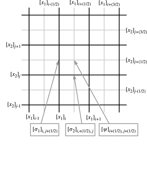
We number cell edges in each of our two coordinate directions, and , by integer indices. The th cell edge in the direction has an coordinate given by , while the th cell edge in the direction has an coordinate given by . The cell centers have coordinates in each direction given by and . Thus, the location of a cell-centers in this mesh is fully specified by a pair of discretized coordinates in the and directions . This staggered mesh is illustrated in Figure 1.
Intensive quantities, such as pressure, mass density, internal energy density, temperature, electron number density (or electron fraction), etc. are defined at cell centers. Components of vector quantities, such velocities, momenta, gradients of intensive quantities, and fluxes are defined on the corresponding cell faces. We refer to these latter quantities as face-centered variables. The spatial location for each of these types of variables is depicted in Figure 1. Note that we use standard subscript notation to define the discretized analogs of all quantities, e.g., is the discretized temperature variable defined at coordinates . Our finite difference notation is described in Appendix A.
It is clear from Figure 1 that vector components are not co-located at a single spatial point on the mesh. Occasionally, quantities derived from these components are needed at alternate locations, in which case a scheme that averages values from nearby spatial locations is employed to compute values at the needed location. We discuss such averaging on a case-by-case basis when we detail the discretization of the equations.
In order to discretize the spectral variables, we also define a mesh over the energy dimension, i.e., the spectrum of radiation energies. The range of the domain in the energy dimension is discretized into groups, i.e., cells in energy space. The th group has a lower edge with an energy coordinate and the center of the th group has an energy coordinate given by . Discretized spectral quantities, such as spectral radiation energy densities and spectral flux densities, are usually defined at group centers. Since such quantities usually have a dependence on spatial location as well as energy, the discretized analogs of these quantities carry an extra subscript indicating their location in the energy dimension. For example, the radiation energy density at spatial coordinates and energy coordinate is denoted as .
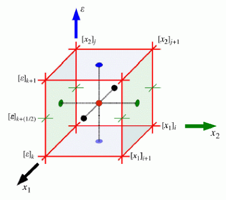
The location of energy-dependent intensive quantities such as the spectral radiation energy density, and energy-dependent vector quantities, such as the spectral flux density are illustrated in Figure 2. A complete listing, delineating where various physical quantities are defined in the spatial-energy meshes, is found in Appendix B.
3.2 Covariant Formulation
We choose to follow Stone & Norman (1992a) by writing all finite-difference expressions in terms of a generalized orthogonal coordinate system that is capable of describing Cartesian, cylindrical, and spherical-polar coordinate systems. Our goal is to enable a single code that is easily adaptable to any 2-D curvilinear coordinate system, avoiding the labor that would otherwise be required to implement a code in each individual coordinate system desired. This technique is well described in (Stone & Norman, 1992a) and we refer the reader there for details. The notation for coordinates and other geometrical quantities that we employ in each coordinate system are described in Table 4, located in Appendix C. The detailed form of the metric coefficients, the gradient and divergence operators, and tensor expressions that are needed to evaluate the radiation-hydrodynamic equations are described in their entirety in Appendices H and J.
3.3 Operator Splitting
Our algorithm employs operator splitting to decouple the overall time integration of the radiation-hydrodynamic equations into substeps. The motivation for this procedure is discussed in Stone & Norman (1992a), to which we refer the reader. In general, we split the right-hand-sides of the time evolution equations into advective, source, viscous, and radiation-matter-coupling terms and solve these split equations to update the hydrodynamic and radiation quantities accordingly.
The following describes the application of this operator-splitting approach to the equations in our model. The time integration of the continuity equation (1) requires no operator splitting, since there is only a single advective term, and no source or collision term, in the equation. Thus, we can restate equation (1) as
| (31) |
where
| (32) |
The electron conservation equation (2) is split into two terms,
| (33) |
where
| (34) |
is the advective term and
| (35) |
is the source or collision-integral term. In a similar manner, the gas-energy equation (3) is split into four separate sets of terms: advection terms, the Lagrangean or source terms, viscous dissipation terms, and the collision-integral terms.
| (36) |
where
| (37) |
| (38) |
| (39) |
and
| (40) |
The gas-momentum equation (4) is operator split into five sets of terms
| (41) | |||||
where the advection term is
| (42) |
the source terms are
| (43) |
the viscous dissipation terms are
| (44) |
the radiation pressure terms are
| (45) |
and the collision integral terms are
| (46) |
Finally, the radiation-energy equation (18) is operator split as
| (47) |
where
| (48) |
while the combination of the diffusive and collision integral terms are defined by
| (49) |
The antiparticle monochromatic diffusion equation (19) is operator split in the analogous fashion to equation (18).
We also note that each of the aforementioned advection terms is itself directionally operator split into two pieces corresponding to advection in each of the two coordinate directions which we generically denote as and . Thus for each set of advection terms we can write
| (50) |
Because of the complexity of the operator split equations, we restrict the discussion of the numerical methods used to solve the individual pieces of the operator equations to Appendices D–L. In the next section we concentrate on the order of updates, based on these operator split pieces, employed to evolve the equations from time to time .
3.4 Order of Solution of Operator Split Equations
Our algorithm employs the following order for solution of the operator-split equations detailed in the previous subsection. The complete sequence of solving each of these operator split pieces constitutes the algorithm for evolving the equations from time to time . A schematic illustration of our algorithm, for a single timestep, is provided in Figure 3. The details of each substep are provided in Appendices D–L. The hydrodynamic portions of the operator-split equations are solved explicitly, while the radiative portions of the equations are solved implicitly. The motivation for this choice of a hybrid explicit-plus-implicit approach is well-described in Stone, Mihalas, & Norman (1992), and we refer the reader there for a detailed description of the issues involved.
Following Stone & Norman (1992a), we denote partial updates of variables of quantities by means of superscripts. Thus, at the beginning of a timestep, the matter internal energy density is denoted by . The partially updated internal energy resulting from, for example, substep (updated via eq. [40]) is denoted by . The superscript serves to indicate that the quantity includes all partial updates prior to and including substep . The final update of each quantity, within a given timestep, is labeled by superscript . When we denote a discretized quantity without spatial- or energy-index subscripts, we are referring to the entire spatial or energy range of that discretized quantity. In our description of each substep, we will describe what quantities are updated as a result of that substep.
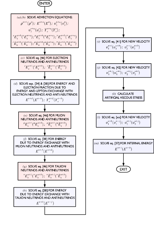
The substep - in the algorithm consists of explicit numerical solution of the advection portions of the operator-split equations. This substep is actually a combination of two directionally split substeps corresponding to advection in the and directions. In this substep, all advective portions of the operator split equations are solved, namely, equations (32), (34), (37), (42), and (48). Note that, since the radiation energy density is a function of spectral energy, equation (48) must be solved for every energy group and for each type of radiation present, i.e., for each of the six types of neutrinos. Thus, equation (48) represents a set of equations that must be solved, while equations (32), (34), (37), and (42) represent five equations (the momentum equation is actually two equations, one for each of the the two components of the velocity). Thus, when the number of energy groups is large, the computational cost of the advection substep is dominated by the cost of solving the radiation-advection equations represented by equation (48). Our algorithm for explicit solution of the advection portion of the operator-split equations is exactly the same as that of Stone & Norman (1992a) and is detailed in Appendix D. We note that after the calculation of the updated values of the radiation energy densities, the Pauli exclusion principal constraint enforcement is applied. This is indicated in Figure 3 by red shading of the advective update box. We also note that the advective update substep is itself composed of numerous substeps in which the advection equations are solved by directionally split substeps. The directionally split advection algorithm utilizes Norman’s consistent advection scheme (Norman et al., 1980) in which the advection of all quantities is tied to the mass-flux. The details of the advection substeps are illustrated in Figure 28 (see Appendix D), to which the reader is referred for more detail. The net result of this substep are the partially updated quantities , , , , , ,, , , , , and .
The second and third substeps (substeps and ) in the solution of the operator-split equations involve the evolution of equations describing the radiative evolution of electron neutrinos and antineutrinos and the exchange of energy and lepton number between matter and these neutrinos. This substep involves the implicit solution of the set of radiation diffusion equations for electron neutrinos and antineutrinos represented by equation (49) and the collision-integral equations represented by equations (35) and (40). In the second step, represented by the second box () in Figure 3, the complete set of implicitly differenced diffusion equations for electron neutrinos and antineutrinos represented by equation (49) is solved simultaneously via Newton-Krylov iteration. The details of the finite-differencing and numerical solution of these equations is detailed in Appendix H. Once the implicit solution of this set of equations has been accomplished, the amount of lepton and energy exchange between matter and electron neutrinos and antineutrinos is fixed. After the new values of the electron-neutrino-antineutrino energy densities are calculated, the Pauli exclusion principal constraint enforcement algorithm is applied to the electron-neutrino-antineutrino energy densities. The application of this constraint-enforcement algorithm is indicated by the red shading of the second box () in Figure 3. The second substep results in updated quantities , , , and fully updated radiation quantities and .
In the substep (represented by the third box [] of Figure 3), since the amount of energy and lepton exchange with matter has been fixed by the previous substep, equation (35) is solved for the new value of electron number density and, thus, the new value of electron fraction . Subsequently equation (40) is solved implicitly for the new value of internal energy density. Once the new internal energy density is determined, the equation of state determines the new value of matter temperature and pressure corresponding to the new internal energy density. The details of this substep are described in Appendix H. The third substep results in the fully updated quantities , , , , and .
The second and third substeps (substeps and ) are subsequently repeated for the muon neutrinos and antineutrinos in substeps and (shown as boxes and the flowchart) and tauon neutrinos and antineutrinos in substeps and (shown as boxes and in the flowchart). In substeps and , the Pauli exclusion principal constraint algorithm is applied to the muon neutrino and antineutrino energy densities and the tauon neutrino and antineutrino energy densities, respectively. This is indicated by the red shading of the boxes corresponding to substeps and in Figure 3. In substeps and , the solution of equation (35) is not required since the production of muon neutrinos and antineutrinos and tauon neutrinos and antineutrinos results in no change in lepton number—these neutrinos are always produced in particle-antiparticle pairs. Equation (40) is solved for the new matter internal energy density, temperature, and pressure, as described in the case of the second substep. Substep results in the updated quantities , , , , and . Substep results in the updated quantities , , and . Substep results in the updated quantities , , , , and . Substep results in the updated quantities , , and .
In substep , the momentum and velocities are updated via the solution of equation (43) to account for gravitational- and pressure-induced accelerations. This substep is almost identical in detail to that of Stone & Norman (1992a), but we describe this in detail in Appendix F. In this paper, we consider the gravitational force to be spherically symmetric based on the mass constained interior to a given radius. The description of the calculation of the gravitational mass is also detailed in Appendix F. This substep results in the updated quantities and .
In substep , the momentum and velocities are updated via the solution of equation (45) to account for radiation-pressure-induced accelerations. This substep relies on the Eddington factor differencing of the gray transport algorithms of Stone, Mihalas, & Norman (1992) and Turner & Stone (2001) which, for our multigroup transport, is applied on a group-by-group basis. We described this approach in detail in Appendix J. This substep results in the updated quantities and .
In substep , the components of the artificial viscous stress are calculated according to the prescription of Stone & Norman (1992a). This calculation is described in Appendix E.
In substep the momentum and velocities are updated via the solution of equation (44) to account for accelerations induced by the gradients of the viscous stress. This substep is identical in detail to that of Stone & Norman (1992a), and we describe this in detail in Appendix E. This substep results in the updated quantities and .
In substep , the internal energy density is updated via the solution of equation (39) to account for viscous dissipation. Like substep , this substep identical in detail to that of Stone & Norman (1992a), and we describe the update equation in Appendix E. This substep results in the updated quantity . We point out that the temperature and pressure are not updated in this step, as they will be updated after the following step.
In substep , the Lagrangean portion of the gas energy equation, described by equation (38) is solved to account for compression or expansion of the gas and the effects of viscous stresses. The time differencing of this equation is implicit. However, the since the divergence of the velocity in equation (38) is evaluated based on the partially updated velocities , there is no spatial coupling between the unknowns in equation (38). This equation can thus be solved by a local, nonlinear iterative solution algorithm in each spatial zone. The finite differencing of equation (38) and our solution algorithm are described in Appendix G. This substep results in the updated quantities , , and .
This sequence of partial updates represented by substeps to constitutes the algorithm for evolving the equations of neutrino radiation hydrodynamics from time to time .
3.5 Boundary Conditions
Up to this point, we have neglected any discussion of boundary conditions and how they are applied within the algorithm. In general, boundary conditions for a specific quantity are applied immediately after any update of that quantity. Thus, any given quantity may have boundary-condition updates several times during the course of a single timestep. The details of how specific boundary conditions are applied are delineated in Appendix K, and we refer the reader there for more information.
In a parallel implementation of our algorithm, where parallelism is achieved via spatial domain decomposition, there are also internal “processor boundaries.” Values of variables at these boundaries must be kept consistent among processors. Thus, boundary updates are a frequent occurrence, since internal processor boundaries are in the middle of actively computed regions. Such consistency requires update of values of a quantity at the edge of processor boundaries after each update of that quantity—before it is needed for another calculation requiring spatial derivatives of that quantity. We discussion this issue in §3.8.
3.6 Timestep Selection
The stability of our algorithm is restricted by the stability of the solution of explicitly solved operator-split equations. In calculating the timestep we follow the algorithm laid out in Stone & Norman (1992a). This algorithm for selecting the timestep depends on several different types of stability criteria which are then combined as an RMS average to yield a stable timestep.
The calculation of the timestep is based on four key criteria. The first is the Courant timescale (calculated in both the and directions), which represents the minimum sound-crossing time for a particular zone in each dimension. More formally,
| (51) |
where is the local speed of sound at coordinate (). An accurate calculation of requires the equation of state to supply an adiabatic index. For the purposes of timestep selection, however, a conservative overestimate of is obtained by making a conservative approximation (i.e., overestimate) of the sound speed by using a polytropic EOS having an overestimate of .
The second and third metrics are the flow timescales in the and directions, which are the timescales over which a particle in the fluid, located at one cell face, can travel to the opposite face, in each respective direction. These timescales are expressed as
| (52) |
and
| (53) |
Finally, the fourth timescale is a viscous dissipation timescale set by the magnitude of the viscous stress. This timescale is defined as
| (54) |
where we compare the timescales in each direction and take the minimum. The quantity is a number of order unity and is defined in Appendix E.
The inverse squares of each of these timescales are added at each mesh point. The maximum value of the quantity in parenthesis in equation (54) is found for the entire spatial domain. The inverse square root of this quantity represents the minimum timescale in the entire domain. A fraction, which we refer to as the CFL fraction and designate by , of this time is used as the new timestep size. It is our practice to fix throughout the course of a given simulation. Typically, we set .
Thus, the timestep value eventually used is
| (55) | |||||
3.7 Equation of State and Opacity Interface
This algorithm makes no assumption about the equation of state other than assuming that the EOS is of the form
| (56) |
and
| (57) |
Our numerical algorithm can accommodate an arbitrary EOS of this form. The algorithm does not rely on solution of a Riemann problem and makes no assumptions about convexity in the EOS. Thus, the EOS can be supplied as a simple formula that can be evaluated in a small subroutine or, alternatively, in the more general form of a thermodynamically consistent tabular interpolation (Swesty, 1996). The algorithm does require that it be possible for the relationship described by equation (56) be inverted, either analytically or numerically to yield
| (58) |
In particular, whenever a new value of the matter internal energy is calculated, it must be possible to compute a new value of the temperature corresponding to that internal energy. A polytropic EOS can be easily accommodated within the relationships described by equations (56)–(58).
We also assume that the absorption opacity, the conservative scattering opacity, and the emissivity be of the form
| (59) |
| (60) |
and
| (61) |
The absorption opacity and the emissivity should be related in such a manner as to preserve the quantum mechanical principle of detailed balance (see §2.3).
The scattering opacity is assumed to be of the form
| (62) |
where, in the scattering reaction, is the energy of the incoming particle and is the energy of the outgoing particle. This opacity should also preserve detailed balance.
Finally, the pair-production rate is assumed to be of the form
| (63) |
where is the energy of the neutrino that is produced and is the energy of the antineutrino that is produced.
3.8 Parallel Implementation
The size of problem encountered in multidimensional radiation-hydrodynamic models, particularly in stellar collapse, necessitates our use of massively parallel computing resources in order to solve the discretized equations. Since we solve a long-timescale problem, it is necessary that we achieve strong-scaling, i.e., we wish a fixed-size problem to scale well to a large number of processors and, therefore, reduce our wall-clock time to solution. In addition, the number of variables in the problem requires a large amount of memory, further necessitating a parallel solution strategy.
A parallel implementation of our algorithm can be achieved via spatial domain decomposition of the 2-D spatial domain into a logically Cartesian topology of 2-D subdomains. Such a decomposition is illustrated in Figure 4.
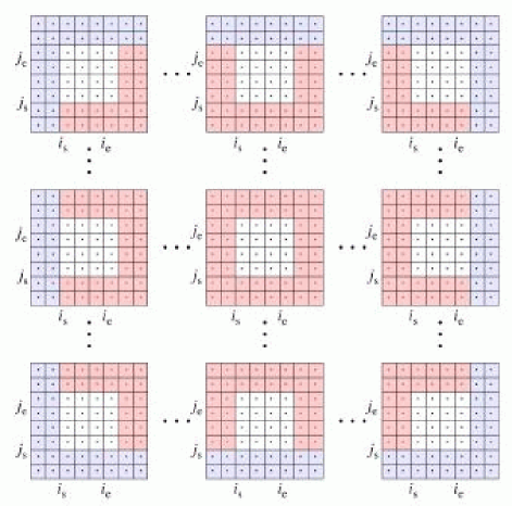
This is a well-established scheme for the parallelization of numerical methods for partial differential equations (Gropp et al., 1999a). The logically Cartesian process topology is straightforward to create using MPI (Message Passing Interface) subroutine calls (Gropp et al., 1999b) and can be configured to allow for periodic boundaries if so desired. This logically Cartesian spatial decomposition is independent of the choice of coordinate system and is carried out with an orthogonal spatial mesh defined by generalized coordinates, which we have described previously. The partitioning of this mesh into subdomains is accomplished by specifying the size of the process topology in each of its two dimensions. Once the size of the process topology has been specified, the mesh is divided in an approximately even fashion over the process topology to achieve a balancing of computational work. By specifying the process topology to be as square as possible, the ratio of the number of ghost zones to non-ghost zones can be minimized, thus reducing the communication-to-computation ratio and improving the scalability of the algorithm.
In our parallelization scheme, we do not decompose in the spectral energy dimension of our mesh. Thus the 2-D quadrilateral subdomains illustrated in Figure 4 are actually 3-D hexahedra, where the third dimension is the spectral energy dimension. By not decomposing the problem in the energy dimension we avoid costly communication that would be associated with the evaluation of the integral terms in equations (24), (25), (27), and (28), as well as the application of the Pauli exclusion principal constraint enforcement algorithm.
Under a logically Cartesian spatial domain decomposition, our discretization algorithms for the hydrodynamic and radiation-transport equations require a limited set of communication patterns. Evaluation of fluxes or spatial derivatives gives rise to a local discretization stencil that requires information from “ghost zones” surrounding each subdomain. The values of variables in these ghost zones must be obtained from adjacent subdomains by means of message-passing to and from nearest-neighbor processes. This process of ghost-zone exchange is illustrated in Figure 5.
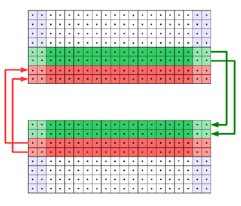
Ghost zone values of a specific quantity, such as density, must be exchanged before those values are needed in the evaluation of any expression in which those variables appear. These exchanges can be accomplished asynchronously, but we avoid discussion of the complexities of doing this, since that topic is beyond the scope of this paper.
The number of the ghost zones required is a function of the discretization scheme. An examination of the finite difference equations, presented in the appendices, indicates that the maximum number of zones that couple within a single equation is five in each spatial dimension. For example, equation (1), for van Leer advection of scalars, couples five zones , , , , and centered about the cell center in the direction. If a spatially higher-order differencing scheme were implemented, there would be longer-range coupling among zones. Therefore, the width of the ghost-zone region would be correspondingly larger. Readers who desire a more complete description of ghost-zone exchange are referred to Chapter 4 of Gropp et al. (1999a). For the implementation of the algorithm described in this paper, two ghost zones in each spatial dimension are required.
Unfortunately, nearest-neighbor message passing is not the only communication pattern required by the algorithm. Global reduction operations are required in two instances. First, calculation of the timestep size, (see §3.6), requires a global reduction to determine the minimum CFL time for the entire domain. Second, the Newton-Krylov-based iterative solution of the implicitly differenced radiation-transport equations (Appendix H), requires global reduction operations to evaluate vector inner products. In the BiCGSTAB algorithm, which we use to solve the linear systems in the Newton-Krylov scheme, this can mean multiple global reductions per iteration. This can impose a bottleneck to scalability for simulations running on large numbers of processors. To reduce this bottleneck, we have developed an algebraically equivalent variant of the BiCGSTAB algorithm, which requires only one global reduction per iteration (Swesty 2006, in preparation). This improvement can be seen in Figure 6, where we plot the parallel speedup of the algorithm when calculating a supernova model on seaborg, the IBM-SP at NERSC.

The major floating point cost of the Newton-Krylov algorithm is expended in the evaluation of the finite-differenced nonlinear diffusion equation. This operation requires only nearest-spatial-neighbor communication to evaluate the finite-difference stencil of the divergence operator. Whenever the nearest neighbor is a zone whose data is resident on another processor, we amortize the communication cost by performing the nearest neighbor-communication asynchronously. This allows us to carry out, simultaneously, the portions of the matrix-vector multiply operation corresponding to interior (local) zones of each subdomain. This yields a further improvement in scalability, as seen in Figure 6.
3.9 Code Structure
Although time advancement is the most important part of the algorithm, it is only the central portion of a sequence of many operations that manage an overall simulation. For completeness, we present a diagram of the remaining portion of the algorithm in Figure 7.
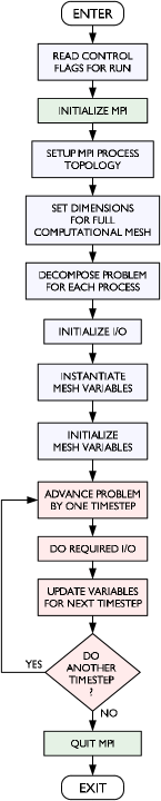
Several of the initial operations, depicted by blue boxes in Figure 7, reflect a parallel implementation of the algorithm. The main computational effort described by the flowchart is the time evolution loop depicted by the red boxes in Figure 7. The core of this loop is the timestep evolution previously described in Figure 3. The purpose of the loop in Figure 7 is simply to evolve the equations forward in time.
Of note in Figure 7 is that we periodically write out data from a run in the form of checkpoint files. These files capture the state of the simulation and serve two functions. They act as restart files, so that a simulation can be resumed from any checkpointed timestep. They also serve as a resource for post-processing analysis. Use of parallel file systems, MPI-I/O (Gropp et al., 1999b), and HDF5222http://hdf.ncsa.uiuc.edu/HDF5/ in our simulations allows us to create a checkpoint file, using a particular number of processors and processor topology, and restart it at a later time, using a different processor count or topology. In fact, it is routine for us to use checkpoint files in this manner. The file portability built into both MPI and HDF5 also allows our use of these files across diverse computer architectures.
4 Code Verification Tests
To test our algorithm, we have subjected the code that implements it, V2D, to a suite of verification test problems that stress individual components of the code in a variety of different contexts. These tests are broken out into five main classes: (1) hydrodynamic tests, which test only hydrodynamic portions of the code, i.e., without radiation transport; (2) gravity tests, which also involve hydrodynamics, but which stress self-gravity of the system; (3) transport tests, which test the radiation transport portion of the code, but in a static medium (i.e., without hydrodynamics); (4) radiation hydrodynamics tests, which test the coupled hydrodynamic and radiation portions of the code; and (5) correctness and scalability tests, which are a diverse set of tests used to test such things as the nonlinear solvers implemented within the code and the correctness and scalability of the parallel implementation of the code.
Because of the length of this manuscript, we have chosen only a few problems for each of these categories. These problems were chosen to encompass the most important aspects of algorithm correctness. In some categories, such as hydrodynamics, there are many classic verification test problems that we have not included for reasons of brevity. All of the test problems we have included in this section, along with many others, are run as automated regression tests that are executed daily against our source code repository.
In the following subsections we provide verification test descriptions and results for each of the aforementioned categories.
4.1 Hydrodynamic Tests
The hydrodynamic verification tests we have implemented employ solely the hydrodynamics aspects of the algorithm. These problems only involve equations (1)–(4), as presented in §2.1, with all radiation-coupling terms omitted.
We perform three standard tests of hydrodynamics. The first is a passive advection test, which tests the ability of an advection scheme to preserve features in a the profile of a physical quantity when the quantity is advected by a moving medium. The second and third problems, the shock tube and the Sedov-Taylor blast wave, test a code’s ability to reproduce the solutions to two standard problems whose solutions are known analytically.
Two of these tests, the passive advection problem and the shock tube problem were performed by Stone & Norman (1992a), but since our hydrodynamic algorithm differs slightly in the order of solution steps, we repeat these tests to establish the performance of our algorithm on the classic problems. The Sedov-Taylor blastwave problem was not addressed by Stone & Norman (1992a), and so we include the problem here.
4.1.1 Passive Advection
The passive advection test exclusively exercises advection equations described in Appendix D. The goal of this test is to delineate how faithfully a waveform is preserved as it propagates through a moving medium. Hence, it serves as an excellent measure of the diffusivity of the advection algorithm. For comparison purposes, our setup closely follows the passive advection test results reported in Stone & Norman (1992a). Source terms in the hydrodynamics are ignored and only the advection equations are evolved in time. There are no gravitational forces, no pressure gradients, and no radiation. In Cartesian coordinates, the test uses a uniform, time-independent velocity field, which is set to cm s-1, parallel to one of the axes. As an initial waveform, we set up a square pulse 50 zones wide near the left-hand boundary of a domain 400 zones wide, where each zone is 1 cm wide. This pulse is applied to the density, and since we assume the material is an ideal gas, it also appears in the pressure and internal energy. Specifically, for passive advection in the direction, we set g cm-3 and erg cm-3 in the region cm cm, and g cm-3 and erg cm-3 elsewhere. The velocity in the direction is set to cm s-1 and the velocity in the direction is set to zero. The matter internal energy density is set to everywhere with . These initial conditions are evolved until the pulse propagates a distance of five times its initial width. With the background velocity, and using a timestep of 5 s, this is achieved in 1000 timesteps.
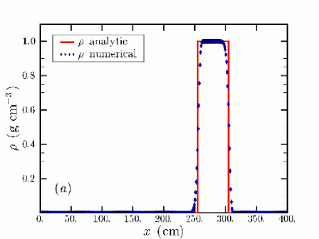
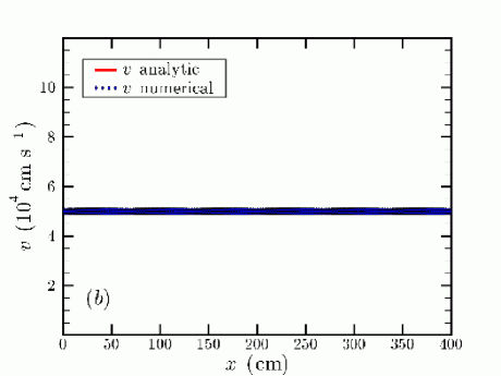
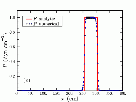
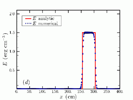
Results for our test are shown in Figure 8. Although there is some diffusion evident, given that the square pulse shape is not preserved exactly, the performance of V2D’s implementation of advection is in good agreement with the results of Stone & Norman (1992a), who have also implemented van Leer’s scheme. We perform numerous variations on this test. In one such Cartesian variation, we run the mirror image of the test in the negative direction. After making the necessary changes to adjust for the symmetry, results of the tests in the and directions are found to be bitwise identical. We also perform the same pair of tests in the and directions. Once again, results of this pair are bitwise identical, mutatis mutandis. This -direction pair also has bitwise identical results to the pair of tests in the direction.
4.1.2 Shock Tube
The shock tube problem serves as an important test of both the advection scheme employed by a code and of the overall performance of a hydrodynamic algorithm. First introduced by Sod (1978), it is now widely used as a standard verification test. Although essentially a one-dimensional problem, it turns out to be a useful test for a 2-D code. This is because, in addition to checking for the correct behavior in the principal direction of interest, it can also check that this correct behavior is exactly replicated at all points in the second dimension.
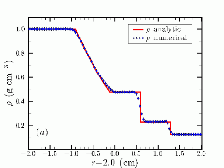
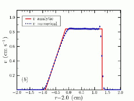
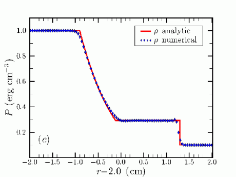
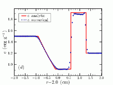
We set up and run the shock tube problem in each of the three coordinate systems (Cartesian, cylindrical, and spherical) and in each direction. For the purposes of this discussion, we choose , where can be related either to the -direction in Cartesian coordinates, the radius in cylindrical coordinates, or the radius in spherical coordinates. We construct the numerical solution with 100 zones in the direction and 12 zones in the direction. As just discussed, the coordinate is centered about zero. It extends 4 cm in total such that . Zones in each direction are uniform in spatial extent. The initial conditions are those set forth by Sod: in the left half of the domain we have g cm-3 and erg cm-3, while in the right half we have g cm-3 and erg cm-3. All velocities are initially zero. The internal energy density is initialized to everywhere. In this, and all the shock tube problems in our test suite, we have set the polytropic index, .
In our tests, we follow the subsequent evolution until . The decision of how long to run the problem differs among authors. For comparison purposes, the particular choice is important only in that the problem needs to run long enough so that the resulting shock wave can propagate a significant distance into the low-density gas. However, the calculation must not run so long that the shock reaches the right-hand boundary of the computational domain. Our choice of timestep size is governed by the CFL condition (see §3.6), and our fraction of the CFL time is set to 0.5. With these choices, each test run takes 59 timesteps to reach 0.70 s. Results for a test run using spherical coordinates are shown in Figure 9. In all our tests, we use our implementation of the van Leer advection scheme combined with Norman’s consistent advection, as described in Appendix D. Our result compares favorably to Stone & Norman (1992a) (cf. their Figure 11). The similarity of these results is not surprising since the hydrodynamic algorithms of ZEUS and V2D have a similar approach, and both calculations use van Leer advection. Our results also compare well to the best results in Hawley et al. (1984b) (cf. their Figures 6–15). In particular, the results using their consistent advection scheme are comparable to those shown here.
In addition to running the shock tube problem in spherical coordinates, as shown in Figure 9, we also perform the shock tube problem in cylindrical and Cartesian coordinates. In the case of the latter, we perform the tests in the and directions and in the and directions. After adjustment for the different coordinate systems and directions, the results of these tests are compared and found to be bitwise identical to each other. As a check of the parallelization of the hydrodynamics algorithm, we also run the shock tube problem in spherical coordinates in the direction on several different processor counts and topologies: a serial (11) single-processor run and parallel 4-, 16-, 64-, and 256-processor runs in 22, 44, 88, and 1616 topologies, respectively. When the results of these runs are compared, they are found to be bitwise identical to each other.
4.1.3 Sedov-Taylor Blast Wave
The Sedov-Taylor blast wave is another example of an idealized problem for which a self-similar analytic solution exists. The solution was originally found by Taylor (1950) and Sedov (1959). The problem is as follows: At time , a large amount of energy is deposited at a single point in an otherwise uniform cold, diffuse, ideal gas. The result is an expanding spherical shock front, behind which is an expanding, spherically symmetric, distribution of matter. Since the solution to the problem is self-similar, there exist similarity variables such that radial profiles of the physical quantities are invariant in time with respect to the similarity variables.
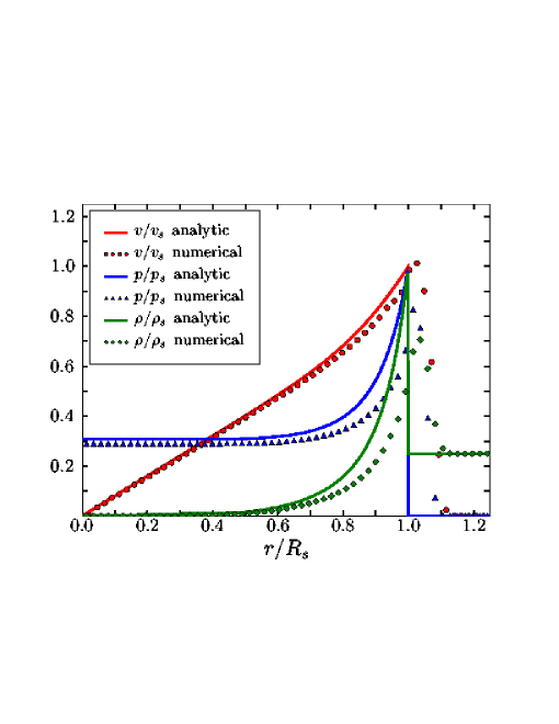
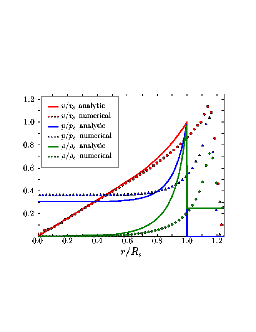
For the numerical test, we set up the problem in spherical coordinates. We choose a spatial domain that is 1-cm in radius and is spanned by 100 uniform width zones in the (radial) direction. In the (angular) direction, the domain size radians with 6 equally spaced angular zones (the number of angular zones should be truly irrelevant to the outcome of the problem). A solution with multiple angular zones is performed purely as a check that the hydrodynamics code is capable of maintaining perfect spherical symmetry. The initial conditions are g cm-3 and MeV. We initialize the problem in two different ways. In the first case we place a high energy density “bomb” of MeV, g cm-3 matter in the the innermost three zones. We refer to this case as the the three-zone bomb case. In the second case, the bomb is located only in the centermost zone and the temperature is set to MeV so as to keep the total bomb energy constant. We refer to this as the one-zone bomb case. The precise values of the initial conditions are somewhat arbitrary as long as the vast majority of the energy in the problem is initially confined to a small region near the center. We assume an ideal gas with . We evolve the solution until a time of seconds using a CFL factor of which takes 1496 steps for the one-zone bomb case and 458 steps for the three-zone bomb case. The results for both cases are shown in Figures 11 and 10. Our results for the three-zone bomb case agree well with other codes where the bomb is spread out over multiple zones. However, the one-zone bomb case is perhaps a more authentic way of initializing the problem which is rarely seen in the published literature. As we can see from Figure 11, the agreement of the numerical and analytic solutions is substantially worse in the one-zone bomb case. The one-zone bomb result can be improved somewhat by using non-uniform zoning.
Defects caused by zoning in numerical solutions of the Sedov-Taylor problem are common. The problem is especially difficult because most of the material piles up behind the shock, and it is difficult to maintain the spatial resolution at all the points necessary to track accurately its movement. Even codes that can draw on adaptive mesh refinement (AMR) still have issues. For example, Fryxell et al. (2000), using the FLASH code, manage to track the position of the shock very well, but are less successful in obtaining good post-shock profiles for the quantities of interest. Pen (1998), also employing an AMR-based code, is forced to choose between optimizing either resolution and positioning of the shock or resolution of the post-shock material.
Finally, we note that when we check our results for spherical symmetry, we observe that the solutions of all radial rays are bitwise identical to each other, and that all velocities in the angular () direction are identically zero at all times.
4.2 Gravity Tests
Although V2D is a code intended for calculations in two spatial dimensions, self gravity is currently approximated by assuming that the mass distribution interior to a point is spherically symmetric (see Appendix F). This treatment naturally leads to gravity verification tests that have spherical geometry. The two gravity verification tests that we consider in this paper (a unit density sphere and a polytrope of index 1), both have spherical geometry and are solved in spherical coordinates.
4.2.1 Unit-Density Sphere
In this test problem we compute the gravitational potential for a sphere of unit density.
Since the gravitational potential given by equation (F9) is a trivial function of the gravitational mass interior to a point, this problem reduces to a test of our algorithm for computing the mass interior to a point. In a serial implementation, this summation could be accomplished trivially. However, in a parallel implementation, this summation requires a series of reduction operations across the process topology. In practice, we accomplish this by first summing the mass in a shell at a given radius by a series of MPI global reduction operations in the direction. Once the amount of mass at a given radius is known, the total mass interior to each radial zone is summed in an outward fashion starting from the inner edge of the grid. These summation steps involve numerous message-passing operations and the purpose of this test also serves to verify the correctness of our implementation.
The problem is set up by constructing a 10-km sphere of unit density, which consists of 100 radial zones of equal spatial width and 40 angular zones of equal angular width, extending from 0– radians. The gravitational mass is computed using the method given in Appendix F. The result is compared against the simple exact computation that is possible for this problem.
The value of this test is the comparison that is possible between the exact method and the various modes of calculation that may take place when V2D is executed. One of the pitfalls in parallel computing is the potential effect in global summation operations caused by floating point arithmetic being neither associative nor distributive. Thus, the answer to a summation operation that is distributed over multiple processors will, in general, produce a result that is dependent on the number of processors used. Furthermore, results can vary slightly from run to run, even on identical numbers of processors, since MPI (which is commonly used for message passing) offers no guarantees about the order of arrival of inter-processor messages. Because of this, the order of individual operations may vary from run to run, possibly producing variable results.
To estimate the magnitude of these effects, we calculate the gravitational mass in a number of different ways and compare each result against the exact result. The deviations of these various results from the exact result are shown in Table 1. In what is labeled “MPI with deterministic reduction” in Table 1, we have replaced the MPI_ALLREDUCE operation in the standard MPI library with one of our own construction. Our version is designed to guarantee an identical order of all critical arithmetic operations, regardless of processor count. As the table shows, the deterministic results agree well with the exact result. As indicated in the table, these deterministic results also agree with each other bitwise, i.e., to the full numerical precision of the system on which they were run. This is to be expected from the deterministic design of these calculations. Although determinism is a desirable feature, it is obtained at the cost of serializing certain key time-intensive portions of the computation. Therefore, it is not a practical method to employ in long-running production calculations.
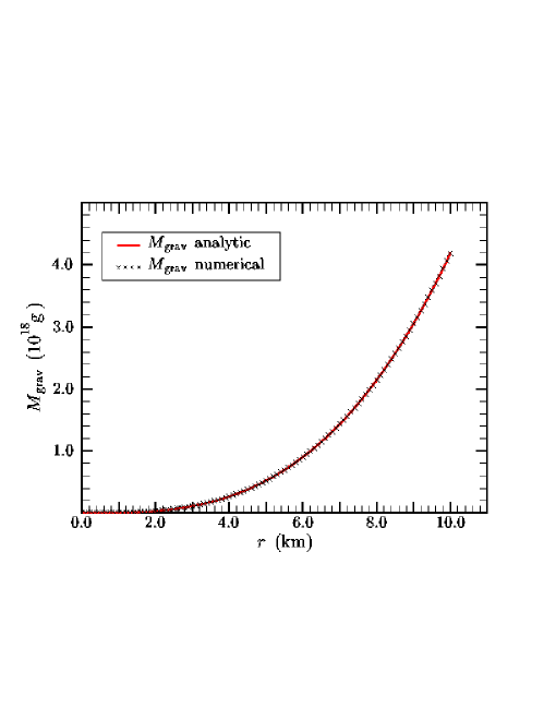
| method used | processor | processor | relative deviation |
|---|---|---|---|
| count | topologyaaProcessor topology dimensions refer to the logical structure by which the two-dimensional computational grid was decomposed among processors, not to any physical processor-interconnect topology that the computer hardware employed. | from exact method b bfootnotemark: | |
| MPI with deterministic reduction | 1 | 11 | |
| 4 | 22 | ||
| 16 | 44 | ||
| 64 | 88 | ||
| 256 | 1616 | ||
| standard MPI | 1 | 11 | |
| 4 | 22 | ||
| 16 | 44 | ||
| 64 | 88 | ||
| 256 | 1616 |
The results in Table 1, labeled “standard MPI,” use the ordinary, standard-compliant MPI libraries for all message passing. Such calculations proceed with no regard to determinism of results. (This is also the mode in which we do production computations using the gravity solver.) The results from this method show, curiously, a smaller deviation from the exact result than shown by the deterministic calculations. More significantly, this deviation differs with processor count, as expected. However, comparisons with the exact result are so good, that it is inconceivable that the overall results of a large-scale, long-running simulation could ever vary in an important way with processor count, solely because of the magnitude of variations exhibited here. Machine epsilon is of the same order () as the deviations—for the architectures on which both these tests and our production runs are performed.
On the basis of these tests, and of others that exercise other parallelized portions of the code (e.g., parallel solvers, the SN tests—see §§4.5 and 4.6), we can proceed with confidence that parallelization alone cannot produce incorrect results (due to mistakes in parallelization) or deceptive results (due to answers that depend on processor count).
Figure 12 shows a comparison of the the exact result and that calculated by the deterministic method using a single processor. As already noted, the agreement is excellent.
4.2.2 Stability of a Polytrope
The polytrope stability verification test involves both gravity and hydrodynamics. This test is initialized by numerically constructing a static polytrope. We then measure how well the static solution is maintained when the polytrope is subjected to hydrodynamic evolution. This test provides a check on both the spherical-gravity solver and on the correctness and stability of the hydrodynamic portion of the V2D algorithm.
We choose a polytrope with index , which corresponds to an polytropic equation of state that has an adiabatic index of . With this choice, we can construct a hydrostatic “star” by solving the Lane-Emden equation, which has an analytic solution for (Chandrasekhar (1967), p. 84ff),
| (64) |
where is the central density and is a radial coordinate defined such that the radius,
| (65) |
where
| (66) |
The quantity is the polytropic constant and is the universal gravitational constant. As indicated by equation (66), for , is independent of . For convenience, we set and choose , such that . Hence, for this problem, the density range throughout this configuration ranges between 0 and , and the surface is located at centimeters from the center.
This analytic solution yields initial conditions for the test problem. We construct a model having 100 radial zones (equally spaced in radius) and 32 angular zones (equally spaced angularly). The zone center coordinates are determined by
| (67) |
in accordance with the coordinate regularization scheme of Mönchmeyer & Müller (1989). To initialize the density, we assign values for at cell centers by averaging the analytic solution evaluated at the adjacent cell faces, i.e.,
| (68) |
This initialization is carried out in an angularly symmetric fashion. Apart from the angular symmetry, we find the exact procedure by which the mesh is initialized to the analytic solution is unimportant to the subsequent evolution.
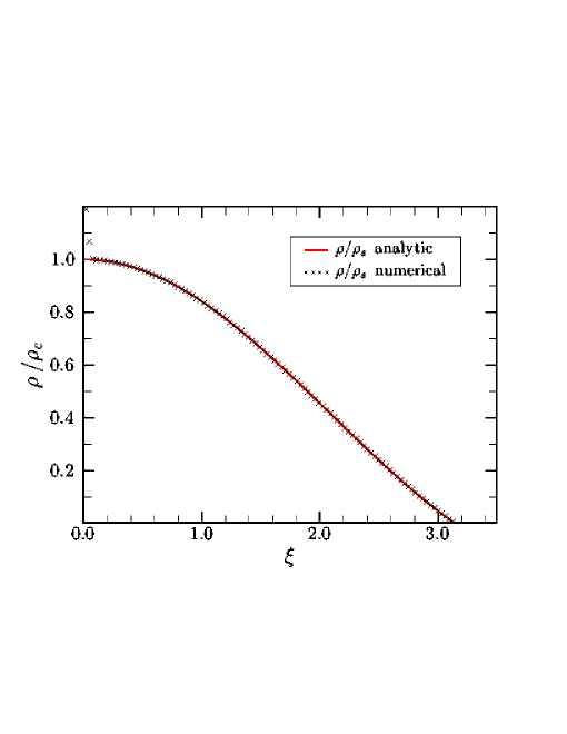
Once initialized, the system is evolved through 1000 timesteps. The timestep size is chosen to have a CFL factor of , as determined by the procedure described in §3.6. After 1000 timesteps, this corresponds to a model time of about 14 500 s. (To prevent the necessity of tiny timestep sizes, given the relatively small angular zone size when using 32 angular zones, we do not include contributions to the Courant time in the angular direction from the first 10 radial zones. To ensure that unphysical motions do not occur because of this, we also suppress all angular motion, that is motion in the direction, inside these 10 zones.)
Figure 13 shows a comparison between the evolved configuration and the analytic solution. Except near the center, where grid resolution is an issue, the numerically evolved solution typically agrees with the analytic solution to a few parts in or better. The larger deviation near the center is a result of gridding effects where the mesh provides insufficient spatial resolution. The radial velocities are also checked. After 1000 timesteps, the absolute value of the radial component of velocity nowhere exceeds . The transverse component of velocity remains identically zero at all timesteps throughout the spatial domain. The previous statement is the equivalent of saying that the code allows all radial rays to evolve in identical fashion—as expected, and as required. Similar results are obtained for the case where we choose cm5 s-2 g-1 and the mass of the configuration is .
4.3 Transport Tests
The transport verification tests are intended to establish the numerical performance of the radiation diffusion aspects of the algorithm. Each of the tests described in this section assume that radiation is propagating through a hydrostatic medium. Thus, the hydrodynamic variables are not evolved. Problems that test coupling of radiation diffusion to hydrodynamics are incorporated in §4.4. In all transport and radiation-hydrodynamic tests, the Pauli blocking factors that appear in the collision integral are retained with . However, the problems are such that the particle occupancies are much, much less than unity and therefore the blocking factors obtain a classical value of unity.
4.3.1 Diffusion of a 1-D Gaussian Pulse
This problem makes use of an analytic solution of the time-dependent diffusion equation in 1-D Cartesian coordinates for the case of a constant diffusion coefficient (Crank, 1980; Butkov, 1968; Riley, Hobson, & Bence, 1998). For initial conditions in the form a Gaussian profile centered at point , the analytic solution to the diffusion equation is given by
| (69) |
where is the initial time from which the problem is evolved, and is the evolution time. The quantity the initial amplitude of the pulse and is the diffusion coefficient. This solution can be used to test the diffusion algorithm in both Cartesian and spherical coordinates. In the case of spherical coordinates the pulse is centered at some large radius such that the plane-parallel limit of the spherical coordinate system is reached.
The initial conditions for the numerical solution are constructed as follows. We use a single energy group of radiation, bounded by 0 and 1 MeV. We use the arithmetic average of the group boundaries, 0.5 MeV, to define the energy at the group center. Since the problem is hydrostatic and there is no emission-absorption, there will be no change in spectral shape. Hence, the details concerning energy grouping are irrelevant. Spatially, we divide the domain into 100 radial zones, covering 1 cm radially, with each zone spaced uniformly. In order to achieve the plane-parallel limit the inner edge of the radial grid is placed at cm. Flat (zero-flux) boundary conditions are applied at the inner and edges of the grid with free streaming boundary conditions at the outer edge. The number of angular zones is arbitrary to the outcome of the problem (each radial ray should evolve virtually identically). We perform our test with 16 angular zones, equally spaced in angle, covering a range of radians and check to make sure the solution in each radial ray is the same. This choice of angular coordinates makes the computational domain in the transverse direction cover about 1 cm and, therefore, gives the domain the shape of a small curvilinear “square.”
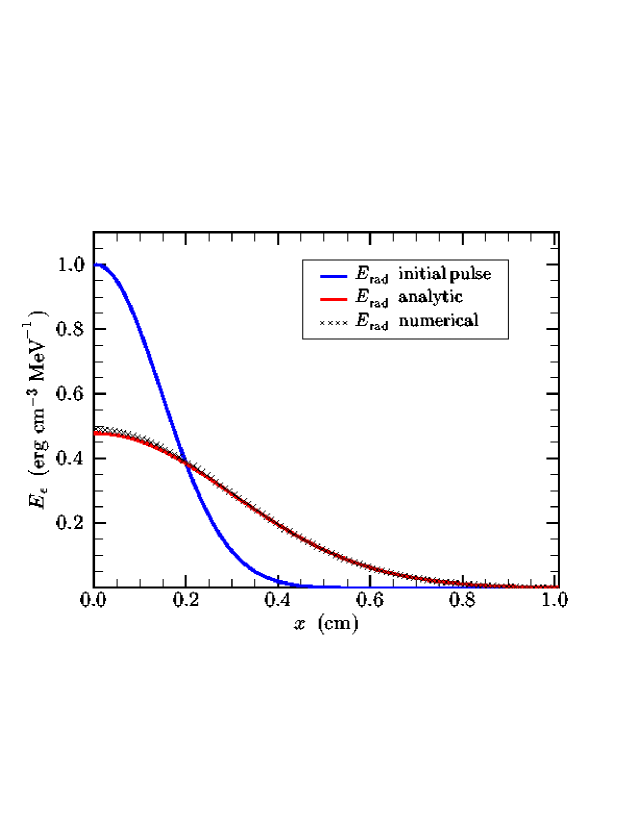
To allow a more complete testing of the code, we perform our calculation by setting up three identical parallel transport problems, thus testing all three species of radiation that V2D is currently set up to track. This is done for both particles and antiparticles of each species. In the language of neutrino transport, this is the equivalent of evolving electron, muon, and tauon neutrinos and their antiparticles. This makes in the equations below have values from 1 to 6, inclusive.
The discretized initial profile is given by
| (70) |
where, as indicated, the radial profile is replicated over all angular zones, and applied to all species of radiation. Here, for the single energy group of radiation being evolved. We have set the diffusion coefficient cm2 s-1, which in the diffusive limit corresponds to a total opacity, cm-1 via equation (9). The constant erg cm-3 MeV-1. After evolving for a time , the analytic solution to this problem leads us to expect a numerical solution of the form
| (71) |
where we have set ns for this test. We run the simulation to where ns, a total of 100 timesteps. The timestep size was chosen to be . Figure 14 shows a comparison between the analytic solution and that achieved by the numerical test. Except near the center, where the numerical solution slightly lags the analytic solution, the agreement is excellent. With the setup described, and using the familiar Euclidean norm, the test exhibits a small relative residual at the final timestep,
| (72) |
for each radiation species individually. As a check, we confirm that the results for each species are bitwise identical.
We also check how well the code maintains spherical symmetry. Because the metric tensor, when using spherical coordinates, contains trigonometric functions of the angular coordinates, it cannot be expected that spherical symmetry will be identically preserved. In our 16-angular-zone model, we find that the maximum relative deviation in the radiation energy densities between corresponding points along radial rays is 4 . Thus, spherical symmetry is well maintained, and the departure from it is of the degree expected for a system whose machine epsilon is of order .
4.3.2 Diffusion of a Gaussian Pulse in Two Dimensions
This problem extends the 1-D Gaussian pulse problem to two dimensions and tests the performance of the diffusion algorithm in multiple dimensions. The computational domain is similar to the spherically symmetric problem: The same single radiation-energy group extending from 0–1 MeV is used. The spatial domain is a curvilinear square similar to that used in the previous problem, but this time measuring 2 cm on a side. The center of this domain is located at a radius of cm from the origin in a spherical-polar coordinate system. The radial domain is divided into 101 zones; the angular domain of rad is also divided into 101 zones. The use of an odd number of zones ensures that the pulse can be placed at the exact center of the domain. Since the computational domain is small relative to its distance from the origin, it resembles a Cartesian grid, which is the way we view it in Figure 15, which shows both initial conditions and results. Nevertheless, the numerical problem is actually solved in spherical polar coordinates and the solution is compared against the analytic solution in that same coordinate system.
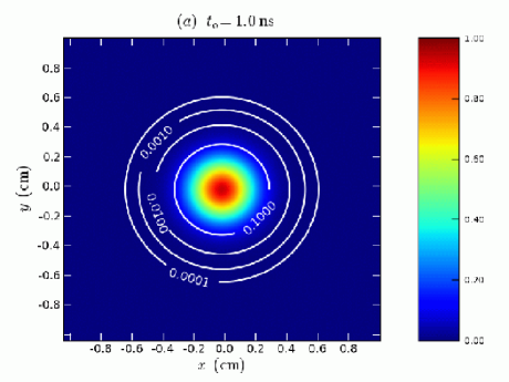
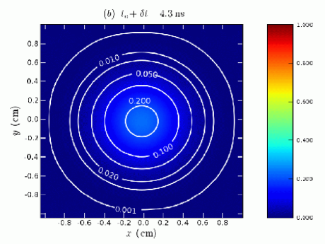
The initial Gaussian pulse is given by
| (73) |
which gives an azimuthally symmetric distribution about the point , which is the displacement of the center of the pulse from the origin. For our test problem, we have selected cm and the direction of the displacement to be located at the angular center of our chosen domain. Once again, we have chosen a uniform, constant diffusion coefficient cm2 s-1, erg cm-3 MeV-1, and ns.
This pulse is initialized numerically at time to the values given by
| (74) | |||||
where is half of the angle subtended by the computational domain at the origin, is the angular coordinate at the first half-integer mesh point, and is the angular coordinate of a general cell center where the distribution is being initialized. The quantity is the angular coordinate of the center of the initial pulse. Flat (zero-flux) boundary conditions are applied at the edges of the grid. We allow the initial pulse to evolve for 3.3 ns in time. As in the 1-D problem, the timestep was chosen to be . By direct substitution, it is straightforward to show (Riley, Hobson, & Bence, 1998) that at time , the analytic solution for this problem is
| (75) |
We note that for this two-dimensional problem, the fraction containing and , which multiplies the Gaussian function, appears as a linear power. This contrasts with the 1-D case, where this factor appears under a square root (eq. [4.3.1]).
The analytic solution corresponds to a predicted numerical solution of
| (76) | |||||
Figure 15 shows the results of solving the test problem numerically with V2D. In Figure 15(a), we show the initial conditions as given by equation (74). Both the colormap and the plotted contours show the initial radiation energy density.
Figure 15(b) shows results after ns of evolution using the same scaled colormap for as in (a). The initial pulse has spread. Except for areas close to the boundary, where edge effects are present, the pulse precisely maintains its axisymmetric form about throughout the evolution. The boundary discrepancies result from our imposition of flat boundary conditions (see Appendix K) and our use (by necessity!) of a finite domain. This results in a numerical solution that is too small at the boundary. The behavior of the solution near the boundaries could likely be improved through the imposition of time-dependent boundary conditions. Nevertheless, at 0.1 cm inside a boundary, the deviation of the numerical from the analytic solution is already reduced to 1.4%, which is typical of the deviation over the rest of the domain. The character of the deviation of the numerical from the analytic solution is similar to the 1-D problem of §4.3.1. The numerical pulse diffuses too slowly, so that it is slightly too large near the center and slightly too small further out.
Running with the setup described and using the results displayed in Figure 15, we calculate the residual as a quantitative measure of the solution quality. With the Euclidean norm, the test exhibits a relative residual at the final timestep of
| (77) |
4.3.3 Flux Divergence Test
The flux divergence test was posed by Turner & Stone (2001) as a means of testing the divergence term of the diffusion equation. Our problem setup is modeled after that test described in §5.2 of Turner & Stone (2001). An analytic solution is known for the case of the diffusion equation on a unit square in Cartesian coordinates with periodic boundary conditions and a constant diffusion coefficient. For this problem, the diffusion equation can be solved via separation of variables. Lamb (1995) outlines an analytic solution:
| (78) |
For the numerical test, we discretize a unit square in curvilinear coordinates into 100 uniform zones in each spatial dimension in a fashion similar to the previous 2-D Gaussian verification problem. The inner edge of the grid is located at cm. For the radiation, we use a single energy group, bounded by 0 and 1 MeV, with the arithmetic average of the group boundaries, 0.5 MeV, assigned as the group-center value. Since this is a pure transport test and the radiation microphysical cross-sections are set such that opacities are independent of material properties (, the values of the material variables are irrelevant (other than the specification that the medium is hydrostatic).
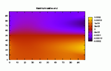
The system is initialized to the differenced form of the analytic solution at a small time, s,
| (79) |
and is left to evolve for 1 second (approximately 100 timesteps). Timesteps are chosen such that , where is the spacing of the radial zones.
The comparison between the numerical and analytical results is very good. Figure 16 shows the maximum relative error of the numerical solution across the spatial domain. This is the maximum relative amount by which each spatial point deviates, at any time, during the course of the calculation. Therefore, at a typical timestep, the solution is actually better than that plotted. In our benchmark calculation, on the final timestep, the maximum relative error that any point reaches over the entire domain is about . The maximum relative error that any point reaches over the entire domain at any time in the course of the simulation is about .
At the final timestep, using the Euclidean norm, we find our results exhibit a very small relative residual,
| (80) |
This number is small at all timesteps throughout the calculation. It sees its maximum value () right at the beginning of the calculation. It then declines almost monotonically to the final value shown in equation (80).
4.3.4 Light-Front Propagation
The light-front propagation problem tests the ability of the algorithm to propagate a front in the optically thin (free-streaming) limit where the behavior of the Boltzmann equation is hyperbolic. This presents a challenging test for a flux-limited diffusion algorithm. This test was used for the flux-limited diffusion algorithm of Turner & Stone (2001) (see their §5.5).
The problem consists of modeling the propagation of a light front, following it from its start, at the inner edge of the domain, until it reaches the halfway point of the domain. The time for this to occur is just the straightforward expectation, based on a front traveling at speed .
The numerical version of this problem is set up in spherical polar coordinates, at a large radius , which we choose as cm. We divide a 1-cm spatial domain in the radial direction into 100 zones, equally spaced. A single radiative energy group is also assigned. It is arbitrarily bounded by 0 and 1 MeV and given the arithmetic average value, 0.5 MeV, at the group center. We set the total radiative opacity, , which is constant in space and time. Like the other transport verification problems in this subsection, there is no emission or absorption. The initial value for the radiation energy density within the computational domain is set to a suitably small value ( erg cm-3 MeV-1) to avoid encountering possible problems with zero or negative energy densities.
Energy is supplied to the domain by a Dirichlet boundary condition at the inner edge of the domain. This is accomplished by fixing all left-hand-boundary zones at all times to 1 erg cm-3 MeV-1. This positions the radiation front at when . Since the problem is of limited duration, the boundary conditions chosen for cm, the right-hand boundary, are largely irrelevant. We run this problem with flat boundary conditions (see Appendix H).
We also run this test as a nominal two-dimensional problem, with 2 zones in the direction that span rad. Periodic boundary conditions are applied to quantities in this second dimension.
These initial conditions are slightly different that those used by Turner & Stone (2001), who fix to achieve an optical depth of 0.01 for the domain. This places our version of the problem in an optically thinner medium, since our smaller value of gives our domain an optical depth of . In addition, Turner & Stone position the radiation front initially at cm.
Our results are shown in Figure 17. This plot corresponds to a time of about s. The curve shown in Figure 17(a) shows results from our standard version of the test. The timestep is selected as 0.5 times the minimum transport CFL time, , in the problem. Since the zones are equally spaced, this corresponds to a timestep of s. The problem runs 100 timesteps to reach the outcome shown. Clearly, the numerical solution is somewhat diffusive.
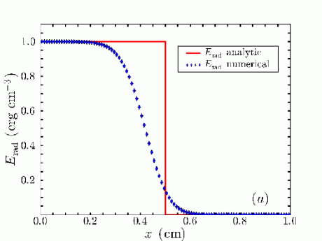
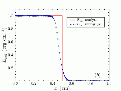
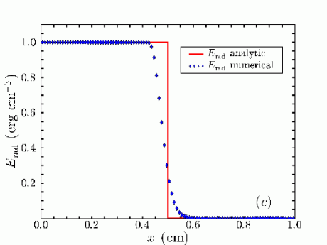
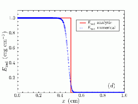
Improvement can be obtained when timesteps are reduced. However, even then, the advantage realized is limited. This is illustrated in Figures 17(b) and (c), where calculations were made using CFL fractions of 0.05 and 0.005, respectively. Although both the radiation fronts are much better resolved than for Figure 17(a), 10 and 100 times the amount of computational effort was expended in producing results (b) and (c) relative to (a). Furthermore, the resolution improvement in (c) relative to (b) is probably not significant enough to warrant 10 times the computational effort.
In Figure 17(d), we set the CFL fraction back to 0.5, but divide the domain into 1000 zones in the radial direction. The combination of more zones, which are thinner and thus decrease the timestep size, results in a calculation that requires roughly the same computational work as performed for (c). The resolution of the radiation front is also comparable, though the increased spatial resolution noticeably sharpens the front and reduces the presence of its numerical precursor.
An analogous set of tests are performed for light fronts propagating in the direction. These tests achieves similar results to those of the direction tests.
All the results we obtain compare favorably with those of Turner & Stone (2001), who also use the Levermore-Pomraning flux limiter in a diffusion scheme to model their radiation. However, in both cases, the diffusivity evident in the solutions demonstrates some ultimate limitations in using flux-limited diffusion in a regime that is maximally far away from the diffusion limit.
4.4 Radiation Hydrodynamics Tests
We have conducted a set of verification tests designed to elucidate the performance of our algorithm on radiation-hydrodynamic phenomena. These tests focus on the exchange of energy between matter and radiation under a variety of conditions. The first of these verification problems tests the exchange of energy in cases where the matter is static. The second tests the exchange of energy under conditions where the dynamics of the matter drives the exchange.
4.4.1 Relaxation to Thermal Equilibrium Tests
This test, suggested by Turner & Stone (2001), is designed to test the ability of a code to achieve thermal equilibrium between matter and radiation by means of emission and absorption. This problem is a gray problem where the emission is blackbody in nature. Our multigroup algorithm can accommodate this problem by simply setting the number of groups to one and setting the group width to MeV. The gray opacities and emissivity can then be used for this single group to model a gray problem. We consider two cases: one where the initial matter temperature is above the equilibrium value and the other where the initial matter temperature is below the equilibrium value. In both cases, the initial radiation energy density is set to erg cm-3. The equation of state is described by a ideal gas with a mean molecular weight of . The density of the material is taken to be g cm-3 and the opacity is taken to be cm-1. In the first case, the initial value of the matter energy density is chosen as erg cm-3; in the second case the initial value is erg cm-3. The timestep was chosen to be s with the initial time set to s. The numerical results of these tests are displayed in Figure 18.
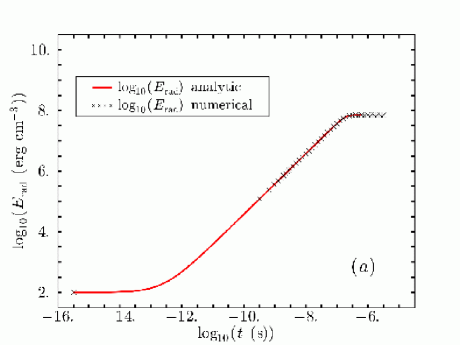
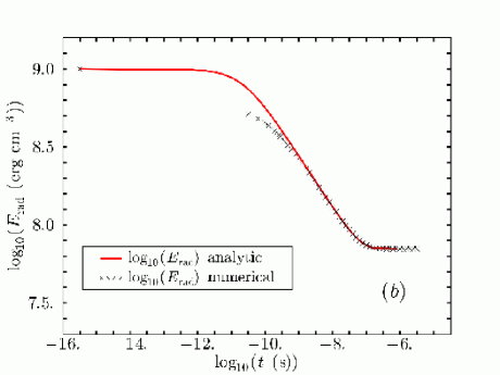
The analytic solution to this problem can be easily obtained by integrating the ordinary differential equation defined by the emission-absorption terms:
| (81) |
where
| (82) |
| (83) |
and is the radiation constant and is the baryon mass. If we make the assumption that the radiation energy density is approximately constant, then by substituting equation (83) into equation (82), we can rewrite (81) as
| (84) |
where and are constants. Clearly, the initial value of the matter energy density , at time , reaches a final equilibrium point at some time . Thus, we can integrate equation (84) to find
| (85) |
The indefinite form of the integral on the right-hand-side of equation (85) can be expressed in two forms (Selby, 1972; Gradshteyn & Ryzhik, 1994)
| (86) |
which depend on the relationship of to . Thus, we can rewrite equation (85) to yield an analytic relationship between and :
| (87) |
In this form, it is easy to compute the time at which a value of the energy density obtains.
In Figure 18, we compare the numerical and analytic solutions that we obtain for both the heating and cooling cases. In both cases, the solution achieves the equilibrium value, as expected. In the radiative cooling case, we note that the numerical results lead the analytic solution slightly for the first few steps. This is expected, since the cooling timescale is initially somewhat shorter than the numerical timestep—resulting in an slightly inaccurate solution. As time evolution proceeds and the matter radiatively cools towards equilibrium, the cooling timescale exceeds the time step, and the numerical solution becomes nearly identical to the analytic solution for subsequent times. The cooling-case result makes an interesting contrast to the results reported in Figure 3 of Turner & Stone (2001), who indicate that their numerical solution for cooling lags the analytic result at early times. The difference between are solution and theirs arises because our algorithm does not solve the Lagrangean portion of the gas energy equation simultaneously with the radiation-diffusion equation.
4.4.2 Radiation-damping of Acoustic Hydrodynamic Waves
This verification test, first carried out by Turner & Stone (2001), is based on the linearized analysis of the radiation-hydrodynamic equations carried out by Mihalas & Mihalas (1983) (hereafter MM83). This analysis predicts the radiation-damping of acoustically driven hydrodynamic disturbances. The dynamics of the acoustically driven wave depend on the ratio of the optical depth of the problem to the damping length.
Our test utilizes the same parameters as those employed by Turner and Stone. The gas is an ideal gas with adiabatic index of . The unperturbed matter density is specified as g cm-3. The unperturbed matter internal energy density is given by erg cm-3 which corresponds to an unperturbed temperature of MeV and an adiabatic sound speed of cm s-1 (). The unperturbed radiation energy density is specified as erg cm-3 MeV-1. We utilize a single energy group centered on an energy of MeV with a width of MeV. This choice of grouping makes the MGFLD equations behave as though they were gray flux-limited diffusion equations. This choice of problem parameters yields a Boltzmann number for the system of
| (88) |
where is the adiabatic sound speed of the gas given by
| (89) |
In the linearized analysis of MM83, the system is also characterized by the quantity given by
| (90) |
which, for the parameters described above, yields the value of . Finally, the matter is assumed to have an absorption opacity given by cm-1.
MM83 posit plane-wave solutions to the linearized radiation-hydrodynamic equations which allows us to write the density, matter internal energy density, and velocity in the form
| (91) |
| (92) |
| (93) |
where , , and are constants specifying the amplitude of the acoustic perturbation.
Based on these perturbations MM83 derive a dispersion relationship for the time-dependent linear radiation-hydrodynamics equations described by the equation
| (94) |
where , , and are complex coefficients given by
| (95) |
| (96) |
| (97) |
and where we define
| (98) |
and
| (99) |
The quantity is related to the optical depth per acoustic perturbation wavelength. MM83 suggest that equation (94) must be solved numerically, but an simple analytic solution of this particular form of quartic equation exists. By the substitution equation (94) is reduced to a complex quadratic equation, for which the standard quadratic formula applies. The roots are then given by
| (100) |
The wave number can then be written as
| (101) |
and, thus, the perturbation takes the form
| (102) |
where the damping length and the perturbation wavelength are defined by
| (103) |
and
| (104) |
The complex relationship between the damping length and the perturbation wavelength is illustrated in Figure 19 for the aforementioned values of and .
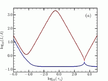
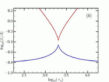
| BehavioraaThe behavior of the material acoustic wave is listed for each set of parameters. | |||||
|---|---|---|---|---|---|
| (rad s-1) | (cm) | (cm) | |||
| damped | |||||
| undamped | |||||
| damped |
This figure reveals that acoustic waves with a values of or should be only slightly undamped while those with should be heavily attenuated. We point out that, despite appearances, the two curves do not intersect near . Our curves, however, show a much closer approach at these points than do the artist-rendered curves of MM83.
To formulate test problems based on this analytic solution of the radiation-hydrodynamic equations, it is more convenient to work with the variable
| (105) |
which is the optical depth per wavelength.
We choose three test cases corresponding to values of of , , and . The corresponding values of and are also given in Table 2. By combining equation (102) with equations (91)–(93), and retaining only the real portion, we obtain the solutions
| (106) |
| (107) |
and
| (108) |
For our test problems we choose the amplitude for the perturbations to be one percent in all cases giving and . The problem is spatially discretized by choosing the zoning such that the domain is divided into 150 zones, with the zone width of 10 zones per perturbation wavelength (). The left-end of the domain is located at a radius large enough to put the spherical coordinate system into the plane-parallel limit. We have retained the same equation of state and energy group structure as used in the radiative heating/cooling problem. The timestep is chosen to be approximately a factor of 10 greater than the heating/cooling timescale in each problem.
The analytic solution describes a wave moving from left to right across the domain. The density, velocity, matter internal energy density, and radiation energy density are initialized to their analytic values at . The perturbations are driven by reseting these quantities to their analytic values in the leftmost ten zones, after the completion of every timestep.
Our numerical results for late-times are displayed in Figures 20–22. The behavior in all cases agrees well with the analytic solution. In the optically thick and thin cases, the numerical solution is damped just as predicted while the optically translucent case produces a solution that is almost unattenuated—again, as predicted. Since the timesteps are much longer than the radiative diffusion timescales, the radiation energy density is essentially flat in all cases. If we choose timesteps shorter than the heating/cooling timescales, we can also reproduce oscillatory behavior in the radiation-energy density.
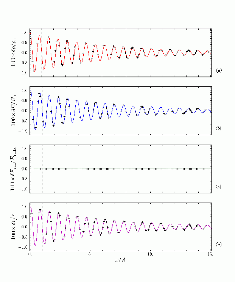
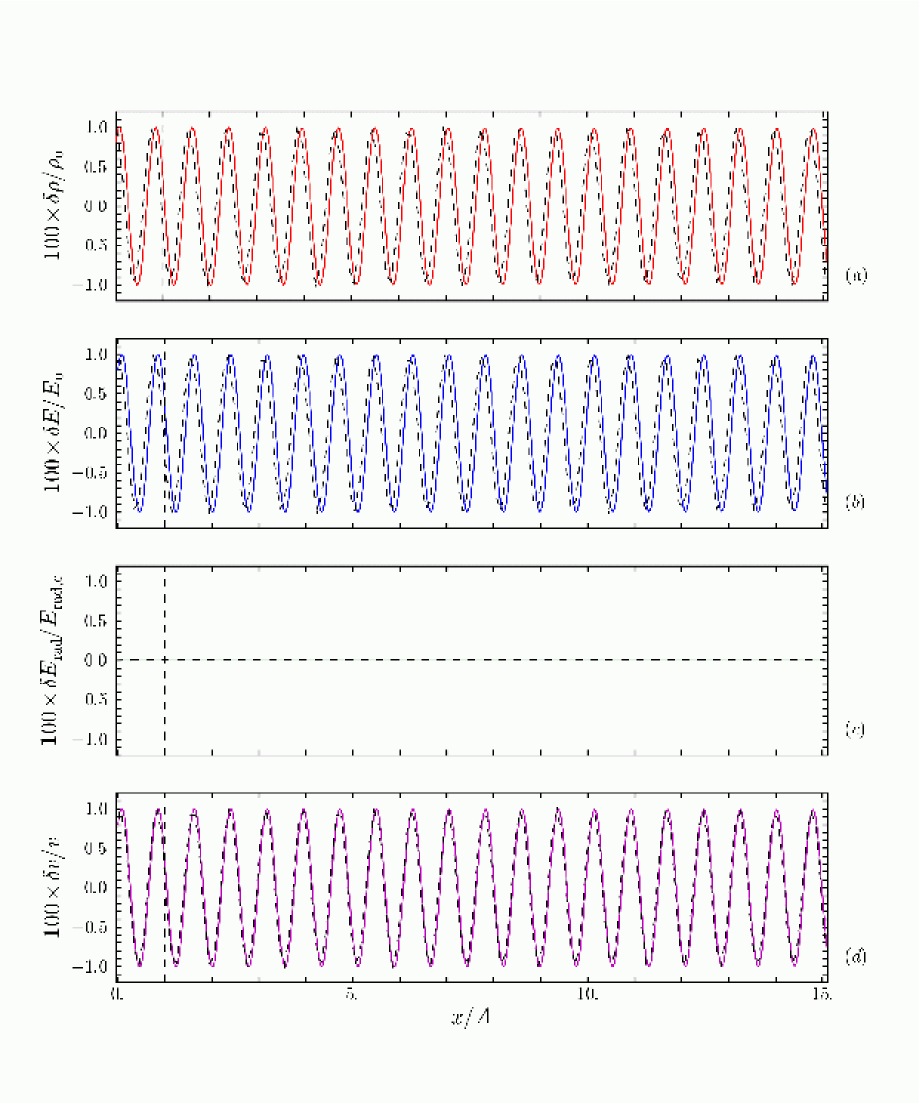
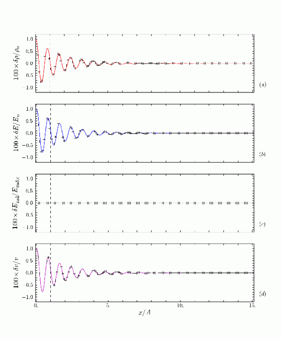
4.5 Parallel-Integrity Tests
The parallel-integrity tests are a set of miscellaneous tests that are intended to confirm that the parallel implementation of V2D is correct. As such, they are more in the nature of computer-code implementation tests instead of physics tests. Nevertheless, since a portion of this paper is devoted to the parallelization of this algorithm, we include a brief description of these tests. The regular execution of these tests is critical to ensure that the parallel implementation is bug-free.
We describe three tests in this section. The first two check for correct parallelization of I/O in the code. The third tests for the correctness of parallelization of the entire V2D code on a test neutrino-radiation-hydrodynamic problem. There are numerous other parallel integrity tests we run that are not described here for reasons of brevity. Although they are described in other sections, we note that the shock tube and unit-density sphere tests described in §§4.1.2 and 4.2.1 are performed in such a way that makes them parallel-integrity tests as well. These tests are run on different process topology configurations and the results are compared to ensure that answers are bitwise identical in all variables regardless of the process topology. In fact, many of our verification tests are likewise run on a variety of process topology configurations and bitwise comparisons are performed among the results.
4.5.1 I/O Process Topology Comparison Test
This test serves as a test of V2D’s implementation of parallel I/O, which uses files formatted in HDF5. An initial HDF5-formatted file is created via a serial program. V2D is rerun multiple times on diverse numbers of processors. Each time, an initial data file is read in via parallel I/O and written back out in parallel. Following this, the output files and input files are then compared to verify that they are identical.
These V2D parallel I/O runs are carried out with several different processor topologies: 11, 22, 44, 88, and 1616, which correspond to 1-, 2-, 4-, 16-, 64-, and 256-processor runs. The processor topology refers to the manner in which the contents of each array have been assigned to a processor. In each case, the data has been decomposed according the spatial dimensions of the arrays. As an example, the 1616-processor run sees a 3232 array divided into 256 portions—each of dimension 22, with one portion resident on each processor. The six distinct output files produced by the multiple runs are compared to each other. We find that these files are bitwise identical, thus providing confidence in the correctness of our parallel implementation of I/O in V2D.
4.5.2 Parallel Memory-File Comparison Test
This test is a variation on the test in the previous section. Whereas the purpose of the “I/O Process Topology Comparison Test” is the integrity of data when different processor topologies are used to do reading and writing, the focus of this test is to confirm integrity of data resident in a file relative to data resident in the distributed memory of an executing parallel program. The two tests also stress two different functional processes by which data is used. The first test stresses a characteristic that is important in the post-processing of production data, which occurs across diverse platforms and processor counts. This second test stresses a characteristic that is important to the checkpointing, suspension, restarting and reading of checkpointed data during the process of performing a single production run.
A parallel program instantiates three four-dimensional arrays of dimension 402132132, which are initialized to specific floating-point values and written to an HDF5-formatted file. The file is subsequently read back by the same program, and the data read from the file is compared to data resident in memory. This test is performed with the same set of processor topologies that are used in the previous test. The decomposition of the data is also handled in the same way. In all cases, we find that the data in memory and data written to files agree bitwise.
4.5.3 Neutrino Radiation-Hydrodynamic Process Topology Comparison Test
The final parallel-integrity test we perform is a test with the complete neutrino radiation-hydrodynamics algorithm. This test stresses all parallel aspects of the code—message passing and global operations in the hydrodynamic and transport sections of the code, and parallel I/O of a realistic data set.
The test is simply constructed. For initial conditions, we take a checkpoint file from a supernova model. The test is conducted by evolving the model forward in time by a single timestep on a number of different processor topologies using a deterministic global reduction operation for global summations. As we discussed in the gravitational unit-sphere-verification-test section, the standard MPI_ALLREDUCE global reduction summation operation is non-deterministic and can yield slightly different answers with each run. Therefore, for testing purposes, we use a deterministic global summation operation. We wish to emphasize that the use of MPI_ALLREDUCE for calculating a global minimum CFL time is deterministic and there are no run-to-run variations in this quantity. For the test, a final output file is produced by each run with varying process topologies. The test is deemed successful if all variables in the checkpoint files are in exact bitwise agreement.
The deterministic global summation operation that we employ uses a brute force approach in which all of the values involved in the summation are systematically communicated to process 0 where they are summed in the same order that they would be summed if the code were purely sequential. Although this approach is slow, it guarantees that the sum is identical to all bits no matter what process topology is employed.
Although impractically slow for production work, deterministic global summations are needed for integrity tests to eliminate the possibility of message passing errors. With the deterministic global sum in place, the output files produced by each processor topology of this test should be bitwise identical. Any deviation indicates a programming error in the parallel implementation of the algorithm. Hence, deterministic programming is an invaluable development tool in achieving and maintaining consistency and correctness of code.
In performing this test, we set up the problem in spherical coordinates with 256 radial zones, 32 angular zones, 20 neutrino groups for each flavor of neutrino and corresponding antineutrino. V2D is then run for a single timestep using a number of processor topologies: 11, 22, 44, 164, 328, where the first number indicates the number of processors across which the radial portion of the domain is divided, and the second number is the same for the angular portion. A standard V2D checkpoint file is written at the end of each of these runs and compared. With the deterministic global reduction in use, we find that all result files are bitwise identical.
4.6 Solver Tests
The Newton-Krylov solver algorithms used to solve the implicitly discretized radiation-diffusion equations are also subjected to regular verification and unit testing. We construct nonlinear and linear test problems that are mathematically simple and for which solutions are known. The solvers are then tested on these problems and the numerical solution is compared to the known solution to ensure that they agree within acceptable tolerances. These tests are carried out on a single processor runs and with multiple processors. The solutions are compared with the known solutions in both cases in order to ensure that no parallel implementation errors are present. We also have carried out numerous tests using both MPI_ALLREDUCE calls and our own deterministic global summation to ensure that the slight process-to-process variability present in the summation of the MPI_ALLREDUCE poses no problem for the solution of the implicit systems arising from the implicitly discretized radiation-diffusion equations. We have never found any physically significant difference in result between the two methods for global summations.
5 Conclusions
We have developed a numerical algorithm for 2-D multigroup neutrino-radiation-hydrodynamics that is especially suited to modeling stellar core collapse, core collapse supernovae, and proto-neutron star convection. However, this algorithm is sufficiently general as to be useful for a variety of 2-D radiation-hydrodynamic applications involving radiation other than neutrinos. Our algorithm solves the combined set of comoving-frame neutrino-radiation hydrodynamics equations, where radiation is treated in a multigroup flux-limited diffusion approximation. The combined set of equations is evolved in time using an operator-splitting approach. The nonlinear diffusion equations are evolved implicitly in pair-coupled fashion while hydrodynamic portions of the operator-split equations are evolved explicitly. The explicit portion of this approach draws on a numerical scheme developed by Stone & Norman (1992a) and Stone, Mihalas, & Norman (1992). The implicit differencing of this scheme is motivated by the work of Turner & Stone (2001). However, the multigroup treatment of the radiation distribution, the pair-coupling between particles and antiparticles, the Pauli blocking effects, the solution of implicitly differenced diffusion equations via Newton-Krylov iteration, and the means of including an arbitrary equation of state have not been heretofore addressed in such an algorithm.
The numerical scheme has been described in sufficient detail to allow a complete implementation of the algorithm by the reader. We have discussed it’s parallel implementation on distributed memory architectures via spatial domain decomposition. This includes message-passing strategies to enhance the scalability of the algorithm.
In order to benchmark the numerical performance of the algorithm, we have presented the results of a suite of important verification tests. These tests stress diverse portions of the algorithm and include hydrodynamic, radiation-transport, radiation-hydrodynamic, gravitational, and parallel integrity tests. Our objective has been to establish the numerical accuracy of our algorithm both as a whole and by individual aspects. This verification process is vital to establish the integrity of future simulations. This process also helps insure that simulations carried out with this algorithm can be properly evaluated by other researchers.
Appendix A Finite Differencing Notation
All discretized quantities are denoted by the use of square brackets around the symbol for the quantity. The location in time at which quantities are defined are denoted through the use of standard superscript notation and is described in §3.4. The location at which a discretized quantity is located in space or energy is denoted through the use of standard subscript notation as follows. Any subscripts inside the square bracket denote a component of a vector, tensor, metric coefficient, or a spectral (radiation-energy-dependent) quantity. energies.Any leading superscripts inside a square bracket are used to label the specific flavor of neutrino-related quantities, e.g., electron, muon, or tauon flavors.
A coordinate, or a quantity derived from a coordinate, which we generalize by , is naturally defined either at cell centers or at cell edges in each dimension. We enumerate cell edges with integer values and cell centers with half-integer values in each dimension. With this convention, cell center is surrounded by cell edges and . Figure 1 illustrates the 2-D spatial mesh, including the enumeration of cell edges and cell centers in each dimension. The spectral or radiation dimension uses an identical enumeration (see Figure 2).
Discretized coordinates are denoted by a single subscript. Therefore, our notation for the discrete analog of coordinate at a cell edge is
| (A1) |
The value of at a cell center is given by
| (A2) |
In these cases, might be spatial coordinates, which we generically refer to as and ; an energy-space coordinate, ; differences of coordinates, metric coefficients, , , and or their spatial derivatives; or the area and volume elements, and , respectively. We use the terms “group” or “energy group” synonymously to refer to cells in the spectral dimension. Usually when we use the terms “cell” or “zone,” we will be referring to the spatial mesh.
In general, scalar quantities are defined at cell centers. A generic scalar quantity , that is a function of spatial coordinates and , has a discretized analog that is notated as
| (A3) |
Figure 1 illustrates the locations for such cell-centered discretized variables. If the scalar quantity is spectral (i.e., a function of the spectral energy ), such as the spectral radiation energy density, we denote it by . The discretized analog of this quantity, when cell centered in the spatial and energy dimensions, is denoted by
| (A4) |
Our convention is that spatial indices follow any spectral indices on all discretized quantities. Figure 2 shows the location at which such quantities are defined in the 3-D (two spatial dimensions and one spectral dimension) mesh.
A general vector quantity, , is decomposed into its two components, and . These quantities are usually defined on the respective cell faces in the direction of the component. Thus, we adopt the following notation:
| (A5) |
| (A6) |
Note that indices inside the square brackets refer to components of the vector. Figure 1 depicts the locations at which the discrete analogs of the vector components are defined.
If the vector quantity is a function of spectral energy (e.g., the spectral radiation flux density), which we denote in general by , and its components by and , then it is face-centered in the spatial dimensions, but group-centered (i.e., cell-centered) in the energy dimension. Thus,
| (A7) |
| (A8) |
Figure 2 illustrates the location at which such quantities are defined.
Most derivatives are calculated via finite differences, and these places will be made obvious throughout the text that follows. For some quantities, however, we calculate derivatives analytically and use these analytic expressions in the code. In the present paper, these analytic expressions are often used for derivatives of the metric scale factors (see §3.2). In differenced expressions, such derivatives are notated as shown in the following example
| (A9) |
Appendix B Discretized Variables
In this appendix, we present a partial list of the more important physical quantities and the discretized notation for these quantities. The conventions for the finite-difference notation we utilize is discussed in detail in Appendix A. The physical quantities and their discretized analogs are listed in Table 3. Figures 1 and 2 show the locations at which these variables are defined.
| Physical Quantity | Algebraic | Quantity Type | Notation |
|---|---|---|---|
| Symbol | |||
| spatial coordinate: cell edge | independent variable | ||
| spatial coordinate: cell center | independent variable | ||
| spatial coordinate: cell edge | independent variable | ||
| spatial coordinate: cell center | independent variable | ||
| spectral energy coordinate: | independent variable | ||
| group edge | |||
| spectral energy coordinate: | independent variable | ||
| group center | |||
| metric coefficient: | function of independent | ||
| cell edge | variable, | ||
| metric coefficient: | function of independent | ||
| cell center | variable, | ||
| mass density | cell-centered, intensive | ||
| electron fraction | cell-centered, intensive | ||
| electron number density | cell-centered, intensive | ||
| matter internal energy density | cell-centered, intensive | ||
| matter pressure | cell-centered, intensive | ||
| matter temperature | cell-centered, intensive | ||
| comp.: matter velocity | face-centered, vector | ||
| comp.: matter velocity | face-centered, vector | ||
| comp.: matter momentum | face-centered, vector | ||
| density | |||
| comp.: matter momentum | face-centered, vector | ||
| density | |||
| spectral radiation energy density | cell-centered, intensive | ||
| comp.: spectral radiation | face-centered, vector | ||
| flux density | |||
| comp.: spectral radiation | face-centered, vector | ||
| flux density | |||
| 1,2 entry: spectral radiation | cell-centered, tensor | ||
| pressure |
Appendix C Generalized Coordinates, Areas, and Volumes
In this section, we describe how the covariant formulation introduced in §3.2 is implemented in our algorithm. In adopting the formulation of Stone & Norman (1992a) for generalized coordinates, we also adopt a portion of their notation. Although there are other possible coordinate systems that could be used with this method, we focus here on the three most common systems: (i) Cartesian, (ii) cylindrical, and (iii) spherical.
Paralleling Mihalas & Mihalas (1984) and Stone & Norman (1992a), we write the metric in a generalized orthogonal coordinate system as
| (C1) |
For Cartesian, cylindrical, and spherical coordinates, Table 4 gives the values of these quantities and their derivatives. In discretized form, these quantities are used both on both the integer and staggered, half-integer mesh.
For Cartesian coordinates , all metric coefficients are unity:
| (C2) |
and all derivatives are obviously zero.
For cylindrical coordinates , the metric coefficients are
| (C3) |
with non-zero derivatives
| (C4) |
Similarly, for spherical coordinates , on the integer mesh, we have
| (C5) |
while on the half-integer mesh, we have
| (C6) |
The non-zero derivatives, when differenced, are
| (C7) |
and
| (C8) |
| Quantity | Symbol | Cartesian | Cylindrical | Spherical |
|---|---|---|---|---|
| coordinates | ||||
| metric scale factors | 1 | 1 | 1 | |
| 1 | 1 | |||
| 1 | 1 | |||
| 1 | ||||
| scale factor derivatives | 0 | 0 | 1 | |
| 0 | 0 | 1 | ||
| 0 | 0 | 0 | ||
| 0 | 0 | 0 | ||
| 0 | 0 | 0 | ||
| 0 | 1 | |||
| decomposed volume elements | ||||
| area elements | ||||
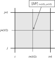
We also make frequent use of the 2-D spatial volume element, , which in general can be decomposed such that
| (C9) |
The decomposed volume elements, the ’s, are given by
| (C10) |
The value of depends on the specific coordinate system.
In Cartesian coordinates, the decomposed volume elements and their discretization are trivial:
| (C11) |
When differenced, they are defined in the code as
| (C12) |
and
| (C13) |
Cell-centered and cell-edge coordinates in the direction are usually related by
| (C14) |
with the analogous relationship for the coordinates. Cell-centered volume elements are also used:
| (C15) |
and
| (C16) |
In cylindrical coordinates, with azimuthal symmetry, these elements become
| (C17) |
which, upon discretization, become
| (C18) |
| (C19) |
Cell-centered and cell-edge coordinates in the direction are usually related by
| (C20) |
with the analogous relationship for the coordinates.
In spherical coordinates, with azimuthal symmetry imposed, these elements become
| (C21) |
When differenced, they appear in the code as
| (C22) |
| (C23) |
We note that writing the volume element in the form used in equation (C22) avoids the computation of the difference of two cubes, which can lead to a substantial loss of precision. The choice of relationship between cell-centered and cell-edge coordinates in spherical geometry is quite important. Following Mönchmeyer & Müller (1989) we usually choose
| (C24) |
for radial coordinates, while choosing
| (C25) |
to relate cell-centered and cell-edge coordinates for the angular dimension. Cell-centered volume elements are also used:
| (C26) |
| (C27) |
Also of importance are the components of the differential area vector, , in the and directions. These are given, in general, by
| (C28) |
Since these elements are components of a vector, these quantities become face-centered when differenced
| (C29) |
and
| (C30) |
Figure 24 shows the location and orientation of the components of these area vectors with respect to the cell volume they enclose.
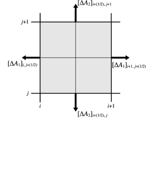
For Cartesian coordinates, the area elements and their discretization are again trivial.
| (C31) |
which, when differenced, give
| (C32) |
and
| (C33) |
In cylindrical coordinates, imposing symmetry in the azimuthal direction, the area elements are
| (C34) |
which, when differenced, give
| (C35) |
and
| (C36) |
In spherical coordinates, imposing azimuthal symmetry, the area elements are
| (C37) |
which, when differenced, give
| (C38) |
and
| (C39) |
Appendix D Discretization of Advection Equations
In this appendix we discuss the solution of equations (32), (34), (37), (42), and (48). Our numerical method for these equations is that of Stone & Norman (1992a) and the first subsection this appendix merely restates their approach for the convenience of the reader. In later subsections we write down the update equations in a convenient form for numerical implementation.
D.1 The ZEUS Advection Scheme
Since equations (32), (34), (37), (42), and (48). have the similar form, we can generalize these expressions. First, for advection of a scalar quantity, we write
| (D1) |
where represents the scalar field being advected. Similarly, for advection of a vector field , we write
| (D2) |
In solving the advection equation, it is common to solve finite-difference approximations to integral forms of equations (D1) and (D2). For advection of a scalar field, this takes the form
| (D3) |
and for advection of a vector field,
| (D4) |
where is an arbitrary volume whose bounding surface is .
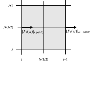
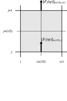
Following Stone & Norman (1992a) we directionally split the update of all equations of the form of (D3) and (D4) into separate sequential updates of the variables due to advection in the and directions. We alternate the directional order of advection updates ( updates followed by updates and vice versa) with each timestep. A complete directional “sweep” is performed by solving all of the advection equations corresponding to one direction, followed by a second sweep solving the equations corresponding to the orthogonal direction.
The consistent advection scheme of Stone & Norman (1992a) ties the advection of all variables to the mass flux. Therefore, we first consider the update to the continuity equation due to advection in the direction. We can write the discretized version of equation (32) as
| (D5) | |||||
where the bounding volume is now , the volume of an arbitrary cell in the computational mesh. The ’s are the areas of the cell faces that, collectively, bound . (These cell-face areas are defined in Appendix C.) The quantity represents the mass flux density (or mass flux per unit area) in the direction across the cell face at . The superscripts indicate the level of temporal update, with being the time-level at the beginning of the advection update, and being the time-level upon completion of the update. If the update is carried out before the update we have and ; if the update is carried out first we have and . The update equation for mass advection in the direction is given by
| (D6) | |||||
where represents the mass flux density direction across the cell face at . As in the update the superscripts indicate the time level at the beginning and end of the update: if the update is carried out before the update we have and ; if the update is carried out first we have and .
Readers who are contrasting our equations with those of Stone & Norman (1992a) will notice that the ZEUS algorithm time-centers many of the quantities that appear in the advection equations. This is necessitated by the possibility that the grid may be moving. Since we are considering only grids that are fixed in time, the advection prescription here is more straightforward. As a consequence of fixing the grid, the spatial coordinates, the volume and area elements, as well as the metric coefficients, are all constant in time.
Simple algebra allows equations (D5) and (D6) are readily solved for the new values of the density in terms of the old values and the mass fluxes which are computed base on those old values.
The mass fluxes are constructed as
| (D7) |
and
| (D8) |
where the ’s are van Leer monotonic upwind advection functions (van Leer, 1977) given by
| (D9) |
where
| (D10) |
and
| (D11) |
Here, and in equations that follow, we have temporarily suspended temporal superscripts whenever writing expressions at a generic time-level. Equations for updates will retain the appropriate time superscripts. For reasons of brevity, we will not write down the analogous expressions for the direction. However, Table 5 gives a complete prescription for constructing from the definition.
The advection equations for scalar quantities other than the density are discretized as
| (D12) | |||||
for the update and
| (D13) | |||||
for the update.
One of the hallmarks of the ZEUS advection strategy is the use of Norman’s consistent advection scheme (Norman et al., 1980), which ties the fluxes for all advected quantities to the mass flux. For scalar quantities other than the density, the fluxes are written as
| (D14) |
and
| (D15) |
When equations (D14) and (D15) are substituted into equations (D12) and (D13) we can solve for new values of all scalar quantities in terms of old values and the fluxes which are calculate in terms of those old values.
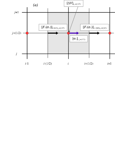
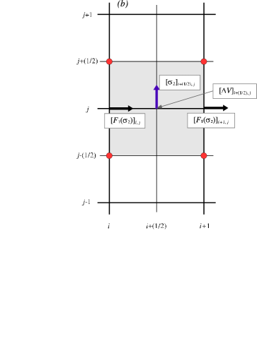
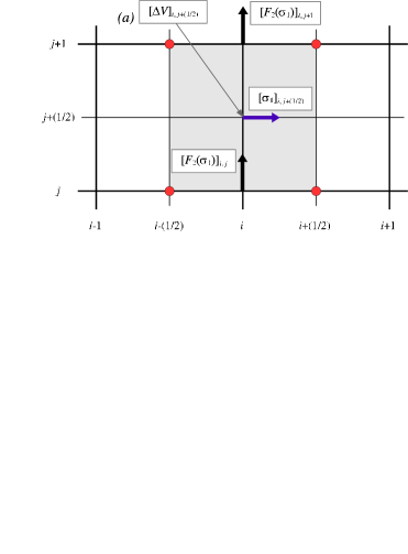
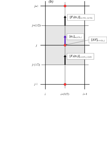
Advection of vector quantities proceeds slightly differently because of the location where vector components are defined on the staggered mesh. The analog of equations (D5) and (D6) for the advection of , the component of vector , in both the and directions is
| (D16) | |||||
and
| (D17) | |||||
where the fluxes are given by
| (D18) |
and
| (D19) |
We note that fluxes in the direction (the ’s) are here needed at cell centers and the fluxes in the direction (the ’s) are needed at zone vertices—locations where neither of these quantities is naturally defined. (Figures 26(a) and 27(a) show the location of fluxes needed to the advect .) We use the following averages to supply the needed values.
| (D20) |
and
| (D21) |
The van Leer interpolation function for advection of the component of a vector in the direction, , is given by
| (D22) |
where
| (D23) |
and
| (D24) |
The interpolation function needed for the calculation of the fluxes in the direction can be obtained by the substitutions described in Table 5.
The analogs of equations (D16) and (D17) for the components of a vector are straightforward to obtain:
| (D25) | |||||
and
| (D26) | |||||
For details we direct the reader to Stone & Norman (1992a). The fluxes are given by
| (D27) |
and
| (D28) |
The van Leer interpolation function needed for the calculation of the fluxes in the direction, , is given by
| (D29) |
where
| (D30) |
and
| (D31) |
The analogous function can be obtained by the appropriate substitutions as described in Table 5.
| Advection Function aaThis column contains the van Leer interpolation functions for advection in the direction that have been provided in full in the text . | Advection Function bbThe deviations shown here for each of the “MPI with deterministic reduction” results, in fact, agree with each other bitwise—they agree to the full numerical precision of the system on which they were run. | Corresponding Substitutions ccThis column contains the needed substitutions in order to use the interpolation functions (eqs. [D9–D11] and [D22–D24]) to construct the functions. |
|---|---|---|
D.2 Update Equations for an Advection Sweep
Using the discretization scheme from the previous subsection and substituting in the appropriate formulae for the cell interface areas, we arrive at a set of update equations for a sweep.
Density update:
| (D32) |
Electron flux:
| (D33) |
Matter-internal-energy-density flux:
| (D34) |
-momentum-density flux:
| (D35) |
-momentum-density flux:
| (D36) |
Radiation-energy-density flux:
| (D37) |
Electron-density update:
Matter-internal-energy-density update:
| (D39) | |||||
-momentum-density update:
| (D40) | |||||
-momentum-density update:
| (D41) | |||||
Radiation-energy-density update:
| (D42) | |||||
D.3 Update Equations for an Advection Sweep
For the advection sweep we obtain the following set of update equations.
Density update:
| (D43) | |||||
Electron flux:
| (D44) |
Matter-internal-energy-density flux:
| (D45) |
-momentum-density flux:
| (D46) |
-momentum-density flux:
| (D47) |
Radiation-energy-density flux:
| (D48) |
Electron-density update:
| (D49) | |||||
Matter-internal-energy update:
| (D50) | |||||
-momentum-density update:
| (D51) | |||||
-momentum-density update:
| (D52) | |||||
Radiation-energy-density update:
| (D53) |
| Direction of First Sweep | Direction of Second Sweep | ||||
|---|---|---|---|---|---|
D.4 Post-Sweep Update Equations
After the advected quantities have been updated during an advection sweep, there are several related updates that must be performed to render certain related quantities, such as the momentum densities and velocities, consistent with one another. The electron fraction should be updated to make it consistent with the electron number density . The two quantities are related by , where is the baryon mass. In discretized form, this becomes
| (D54) |
where after the first advection sweep and after the second advection sweep. We must also update the velocity field that has changed as a result of momentum being advected. This is accomplished as follows
| (D55) |
and
| (D56) |
Finally, the temperature and pressure should be related to render them consistent with the updated density, electron fraction, and matter internal energy density. The procedure for doing this update is the same as that described in appendix I, and we refer the reader there for detail of this procedure. Since the temperature and pressure play no role in the advection equations, we perform this update only after the completion of the second advection sweep. The equation that must be iteratively solved for the new temperature is:
| (D57) |
D.5 The Complete Advective Update
With the complete prescription for the two advection sweeps now derived and differenced, we are finally prepared to assemble the complete sequence of operations of the advection algorithm. This sequence of steps is shown in Figure 28 and corresponds to box of Figure 3. The values for the time superscripts , , , and , which depend on the order of the advection sweeps, are given in Table 6.
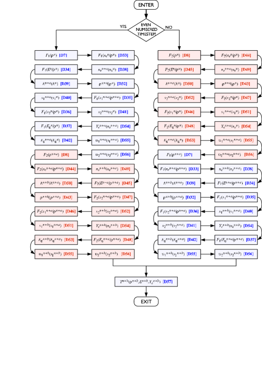
Appendix E Discretization of Viscous Dissipation Equations
To insure the accurate treatment of shocks, the ZEUS algorithm (Stone & Norman, 1992a) includes viscous dissipation in the form of a term that mimics the viscous stresses actually present at a real shock front. Were such a term omitted from our model, the hydrodynamic equations would cause oscillations to develop in the solution. Such oscillations would result from the lack of any means to generate entropy in the finite-difference scheme and satisfy the Rankine-Hugoniot jump conditions across the shock. (For more detail on the choice and implementation of artificial viscosity schemes, see Bowers & Wilson (1991).)
In this work we follow Stone & Norman (1992a), but consider only pseudo-tensorial artificial viscosities. It has been widely known for sometime (Tscharnuter and Winkler, 1979) that tensor artificial viscosities offer superior qualities to scalar schemes. In future work, we will consider such prescriptions, but for now we restrict ourselves to a scalar approach. Readers interested in tensorial forms for the viscous dissipation should consult Stone & Norman (1992a). The ZEUS scheme employs a form of the von Neumann-Richtmyer scheme (Noh, 1987; Richtmyer & Morton, 1967), where the viscous stress in the th direction is given by
| (E1) |
where is a characteristic length. With the substitution of , where is the width of the computational zone in the th direction, we have, upon differencing,
| (E2) |
| (E3) |
By doing this, we have rewritten the characteristic length in terms of a characteristic zone count. For all calculations, we set . The quantity corresponds to the approximate number of zones over which the shock is spread.
These forms enter into the discretized analogs of equations (39) and (44) exactly as described by equations (35)–(37) of Stone & Norman (1992a) and we refer the interested reader there for more detail. We difference equation (39) as
| (E4) | |||||
The components of equation (44) are differenced as
| (E5) |
and
| (E6) | |||||
Appendix F Discretization of Gas-Momentum Source Equation
The solution of equation (43), in substep , accounts for accelerations due to fluid pressure gradients and gravitational forces. Since remains unchanged during this step of the algorithm, it can emerge from the time derivative in equation (43). Thus, we rewrite equation (43) as
| (F1) |
where and are unit vectors in the and directions. Upon differencing, we obtain expressions for updated velocities. In the direction, we have
| (F2) | |||||
where the last term is the contribution of the time derivative of . (The time derivative of yields zero contribution to this term.) The averaging of the nearest four face-centered values of in the – plane gives the value at the need location for calculation of an velocity, viz., at .
Similarly, in the direction, we have
| (F3) | |||||
Here, we note that for spherical self gravity, the component of vanishes. In the case of a general gravitational potential, arising from a non-symmetric solution to the Poisson Equation, a non-zero would be present. In the direction, the contribution of the time derivative of is absorbed into the definition of the velocity. This follows from our definition of , which always has the dimension of length over time, even if the dimension of , itself, is one of angle (see §3.2).
In this algorithm, we assume a 1-D approximation to self-gravity by assuming the mass distribution behaves as if it were spherically symmetric. Although not exact, the highly condensed nature of a collapsed stellar core makes this approximation satisfactory for supernova models. With this assumption of a spherically symmetric mass distribution, we obtain a spherically symmetric gravitational potential of the form
| (F4) |
where is the gravitational mass contained within the radius at time . Note that we we have now specified spherical-polar coordinates for this calculation. Although, this is the most convenient form for problems in spherical geometry, another coordinate system could be used, with the appropriate transformation.
We evaluate as follows. In general, an element of mass is given by
| (F5) |
which in spherical geometry is
| (F6) |
The mass, , is evaluated by performing a radial integral out to the point of interest. When combined with an angular integration, we obtain an angularly averaged mass distribution,
| (F7) |
where the averaging pre-factor in front of the integral allows the computational grid, which runs from to , to be of arbitrary extent—not necessarily reaching either pole.
Finally, the differenced version of these expressions can be written. Note, that although the overall timestep advancement is from times to , since a all quantities that go into the gravitational-potential calculation are evaluated at time , the result is also given a time subscript of :
| (F8) |
with
| (F9) |
We use , and to indicate lower and upper bounds of and dimensions, respectively (see Appendix K). Expressions in equations (F8) and (F9) are evaluated once at the beginning of a timestep and kept constant until the next timestep.
Appendix G Discretization of Lagrangean Gas-Energy Equation
Equation (38) accounts for thermodynamic work done on the fluid internal energy by compression and/or expansion. Our discretization is a generalization of scheme of Stone & Norman (1992a), which allows an arbitrary equation of state in which the internal energy and pressure are expressed as a function of temperature and density. This solution method makes no assumptions about convexity of the EOS.
We implicitly difference equation (38) as
| (G1) |
where the first and third terms of equation (38) contain the EOS in the form of equations (56) and (57), respectively, and where
| (G2) | |||||
For a realistic equation of state, this equation cannot be solved explicitly, since there is no explicit way of expressing matter pressure as a simple function of internal energy. This equation must be solved iteratively for the new temperature , which is unknown and enters parametrically into the new internal energy and pressure through the equation of state as described in equations (56) and (57). Since the solution of equation (38) is the last step in the algorithm, the new value of the electron fraction and density are known prior to the solution of equation (G1). In practice, we employ a combination of Newton-Raphson and bisection algorithms to accomplish the iterative solution of equation (G1). The presence of first-order phase transitions in complex equations of state, such as those describing matter in core-collapse supernovae (Lattimer & Swesty, 1991), can create convergence problems for the solution of equation (G1) Newton-Raphson iteration. These same phase transitions also exhibit non-convex behavior, which can also pose problems for Riemann solver based methods. When non-convergence occurs during the iterative solution of equation (G1), we make use of the slower converging, but more robust, bisection method for single-variable nonlinear equations.
Appendix H Discretization of Radiation Transport Diffusive/Collision Equation
H.1 Pair-Coupling of Equations
In this appendix, we discuss the implicit solution of the sets of diffusion equations for the radiation represented by equation (49). These equations are solved as pair-coupled sets described by boxes (), (), and () of Figure 3. By the use of the terminology “pair-coupled,” we means that discretized version of equation (49) and its antineutrino analog are solved simultaneously for all energy groups for a given type of neutrino (electron, muon, or tauon). For example, in the step represented by box (c) of Figure 3, the nonlinear equations
| (H1) |
and
| (H2) |
are solved simultaneously over all groups for the electron neutrino energy density and the electron antineutrino energy density . There is one such pair of equations for each of the energy groups that span the radiation spectrum. Note that the diffusion coefficients and the source-terms in equations (H1) and (H2) are functions of the neutrino energy and differ between the neutrinos and antineutrinos. The analogous pair-coupled sets of equations are solved in the step represented by box (e) of Figure 3 for the muon neutrino-antineutrino case and in the step represented by box () of Figure 3 for the tauon neutrino-antineutrino case.
For the sake of compactness of notation in the remainder of this appendix, we use the generic notation , without the leading superscripts , , or to refer to the neutrino energy density and , without the leading superscripts , , or to refer to the antineutrino density. The finite-difference equations for each neutrino species can then be obtained by straightforwardly substituting for , for , etc.
H.2 Implicit Finite Differencing of Diffusion Equation
We discretize equations (H1) and (H2) using the spatial differencing scheme developed by Crank (1980) for diffusion equations and using the standard implicit backward-Euler approach for the time evolution scheme. The backward-Euler time discretization scheme has the advantage that method is L-stable for all timesteps (Hunsdorfer & Verwer, 2003).
Equation (H1) is implicitly discretized as
| (H3) |
where
| (H4) | |||||
| (H5) | |||||
and
In equations (H4), (H5), and (H.2) the superscript is used to indicate evaluation of the superscripted quantity at times , and according to whether the equations for electron, muon, or tauon type neutrinos, respectively, are being solved (see Figure 3 for the order of updates). For readability, we have omitted displaying all the explicit functional dependences of the microphysics factors (, , , , ) in the finite-differenced equations. These microphysics factors are also functions of the physical conditions of the matter at the spatial point in question (temperature, density, chemical composition, etc.). In addition, they are functions of the particle energy or energies in the radiation field. We denote this energy dependence in the discretized quantity through the use of additional subscripts:
| (H7) |
| (H8) |
and
| (H9) |
Equation (H.2) is fully implicit in terms of the unknowns and but some of the coefficients arising from the microphysics are evaluated at the beginning of the substep. Following the practice of Turner & Stone (2001), we evaluate the diffusion coefficient and Eddington tensor based on information at the beginning of the substep. The reason for this is that the absolute value function that appears in the evaluation of the Knudsen number would introduce a discontinuity in the Jacobian of the nonlinear system if evaluated implicitly. Such discontinuities can often produce failures in Newton-type iterative procedures for nonlinear systems. By evaluating the diffusion coefficient at the beginning of the substep, we avoid this difficulty altogether. This approximation is accurate as long as the change in the radiation energy density is small over a timestep. For most astrophysical heating/cooling problems, this is indeed the case. In equation (H.2), all quantities that are temperature-, density-, or -dependent are also evaluated at the beginning of the substep. Doing so avoids the difficult problem of simultaneously solving the radiative diffusion equations while also solving the Lagrangean portion of the gas-energy equation. All quantities, such as the opacities, emissivities, etc., are evaluated by using the values of the temperature, density, and electron fraction that are known at the beginning of the substep. If the exchange of energy, or lepton number, that takes place during a timestep is small, this approximation is accurate. The validity of these approximations are tested in the verification problems that we consider in §4.
The antineutrino counterpart of equation (H.2) is given by
| (H10) |
where
| (H11) | |||||
| (H12) | |||||
and
The finite-differenced antineutrino equations (H.2)–(H.2) are almost analogous to the finite-differenced neutrino equations (H.2)–(H.2). The one exception to this one-to-one correspondence is in the pair-production terms where the same discretized function appears in both equation (H.2) and equation (H.2). In the latter, the summation is over the first index of the function, while in the former, the summation is over the second index. Because both and appear as factors in this set of terms, the process of pair-production is responsible for coupling the neutrino diffusion equations to the antineutrino equations. This requires that the two sets of equations be solved simultaneously for each of the three neutrino flavors: electron, muon, and tauon. We discuss the method of solution of these implicitly differenced equations in §H.6.
H.3 Implementation of Boundary Conditions
Boundary conditions are specified for equations (H1) and (H2) by altering the differencing of the and terms. In this subsection, we only present boundary conditions corresponding to equation (H1), with the understanding that similar boundary conditions for equation (H2) can be trivially obtained by substitution of for etc.
We consider three types of boundary conditions in the direction: Dirichlet boundary conditions ( is specified), zero-flux boundary conditions, and free-streaming boundary conditions. The first of these conditions is handled by equation (H4) with no modifications necessary. Zero-flux boundary conditions are usually applied at the inner or left-edge of the grid. To implement zero-flux boundary conditions on a given edge, the corresponding terms in equation (H4) for zones at that edge are set to zero. In the case of free-streaming boundary conditions at the outer (or right) edge of the grid, the corresponding is replaced by in an upwinded sense. Equation (H4) then replaced in the outermost zone by
| (H14) | |||||
In this equation, we have made the assumption that radiation is flowing off the grid at the outer edge in order to determine the upwind direction. This boundary condition must be used with care and only in cases where one is sure of the accuracy of this assumption.
In the direction, we consider three types of boundary conditions: Dirichlet, zero-flux, and periodic. The first of these is again trivial and requires no modification of equation (H4). The second, zero-flux conditions, is treated as we previously described, by setting the appropriate terms to zero in equation (H4) for the zones at the corresponding edge of the mesh. The third case, periodic boundary conditions, is treated by using the ability of MPI to establish periodic process topologies. Using MPI send and receive subroutines to exchange ghost zones, together with a process topology that is periodic in the direction, permits equation (H4) to be used to apply periodic boundary conditions without modification.
Spectral boundary conditions for the term in the direction are handled similarly to the previously described zero-flux spatial boundary conditions. The appropriate terms of in equation (H5) are set to zero at the lower and upper edges of the energy grid. This ensures that no energy flows out of the spectrum at either end.
H.4 Evaluation of Diffusion Coefficient and Eddington-Tensor Terms
In the verification tests described in this paper, we rely on the Levermore & Pomraning (1981) prescription for flux-limiting, which relates the diffusion coefficient and the Eddington tensor to the Knudsen number for the radiation flow. However, the modification of our scheme to utilize other flux-limiters is trivial so long as the diffusion coefficient and the Eddington tensor can be cast into a form that relies on the Knudsen number.
In what follows, we will generically describe the evaluation of Knudsen numbers, diffusion coefficients, and Eddington tensors for neutrinos. The analogous equations for antineutrinos can be obtained by straightforward substitution of for , for , etc., and is not presented here for reasons of brevity.
In our calculation of the diffusion coefficients and Eddington tensor, we emulate Turner & Stone (2001) and make use of separate Knudsen numbers and to describe the radiation flow in each of the two orthogonal coordinate directions. Since Knudsen numbers are based on components of the gradient of radiation energy density, which is defined at cell-centers, the gradients, and hence Knudsen numbers, are naturally evaluated at cell faces—precisely where they are needed. First, for , we have
| (H15) |
expanding the right-hand-side we can write as
| (H16) | |||||
In equation (H16), we have arithmetically averaged the opacities and radiation-energy densities in adjacent cells to obtain values at the zone interface in the direction. The most recent values of the radiation-energy densities, obtained at the end of the advection substep, are used in equation (H16). The values for the opacities are obtained at the beginning of the substep at point , where takes on the values , , or for electron, muon, and tauon type neutrinos respectively. In the direction, an analogous expression can be written
| (H17) | |||||
To obtain the diffusion coefficients in each direction, and , we note that , in the Levermore-Pomraning formalism, is given by equation (11) as
| (H18) |
where is as given in equation (12) and is as given in equation (10). Many other flux-limiting prescriptions can be cast into this form and could easily be accommodated in this algorithm by replacing equation (12) with some other function (see Janka (1991) for a description of how numerous flux-limiters fit this form). Thus, we have:
| (H19) | |||||
| (H20) |
and
| (H21) | |||||
| (H22) |
The evaluation of the Eddington tensor components in terms of the Knudsen number is similarly straightforward. Equations (16) and (17) describe the Levermore-Pomraning prescription for the Eddintgton tensor. The algorithm we present is trivially modifiable to handle other closures replacing these equations with other alternative functions describing the tensor components in terms of the Knudsen number.
We now focus on the components of the Eddington tensor needed to evaluate the tensorial double-contraction terms of equation (H5). This double-contraction can be expressed as
| (H23) | |||||
We have dropped terms that are identically zero in a two-dimensional formulation, namely, those proportional to and .
The components of are evaluated using the expressions derived in Appendix H.5. The required components of are evaluated as follows. Using equation (15), we have
| (H24) |
| (H25) |
| (H26) |
and
| (H27) |
The scalar Eddington factor is evaluated using equation (16), which requires Knudsen numbers, which we have evaluated at cell faces. To perform the evaluation of , which is required at cell centers, we average over the surrounding (directionally decomposed) face-centered values, viz.,
| (H28) | |||||
where we use equation (12) in our evaluation of the ’s.
The factors in equations (H24–H27) containing and arise from the definition of the radiation flux direction . They are evaluated at cell centers by centered differences:
| (H29) |
and
| (H30) |
with
| (H31) | |||||
With the preceding derivations, we now have complete information regarding the differencing of the velocity-dependent terms.
H.5 Velocity Gradients
The evaluation of equation (H23), described in the previous subsection, requires the gradient of the velocity field, . Since is a second-rank tensor, we can use equation (126) in Appendix A of Stone & Norman (1992a) to help with the evaluation. Upon inspecting that equation, it is easy to extract the set of non-zero elements of and obtain
| (H32) |
| (H33) |
| (H34) |
| (H35) |
and
| (H36) |
When differenced, these equations yield the following expressions for the three diagonal elements,
| (H37) |
| (H38) |
and
| (H39) | |||||
The evaluation of equation (H23) requires that components of be evaluated at cell centers. Although this is a natural location for evaluation of the diagonal components of , this evaluation location does not fall naturally for and . Because of cross derivatives, these off-diagonal terms are more naturally evaluated at the vertices of the integer mesh. To obtain the values at the needed locations, we evaluate these expressions using a four-way arithmetic average of the surrounding vertex values, i.e.,
| (H40) |
which, upon use of equation (H35), gives
| (H41) | |||||
Following the same procedure for , and using equation (H36), we arrive at
| (H42) | |||||
H.6 Iterative Solution of the Implicit Finite-Difference Equations
The implicit finite-differencing scheme for the numerical solutions of equations (H1) and (H2) is fully described in the previous three subsections of this appendix. This finite-differencing results in a coupled set of nonlinear algebraic equations that must be solved for the complete set of radiation energy densities for each flavor of radiation. In this section, we briefly describe the iterative method employed to find the solution of this set of nonlinear equations.
The complete set of implicitly discretized equations that must be solved for each radiation flavor is given by equations (H.2) and (H.2). The unknowns in this set of equations are and for ; ; . We use , and to indicate lower and upper bounds of and dimensions, respectively (see Appendix K).
Nonlinearities in this set of equations arise in two forms. First, the pair-production terms in equations (H.2) and (H.2) give rise to a bilinear coupling between neutrinos and antineutrinos if the pair-production kernel is non-zero. This is what necessitates the simultaneous solution of equations (H.2) and (H.2). The second set of nonlinearities are quadratic in form and arise from the Pauli-blocking factors that appear in the scattering integrals in equations (H.2) and (H.2). In the case where the nonlinearities disappear and the set of equations decouples into two separate sets of linear equations: one set describing the energy densities of the radiation particles and one set describing the energy densities of the radiation antiparticles.
In the nonlinear case where and are non-zero, this set of equations could be solved by various means. Because of the sparseness of the nonlinear system, we have used a Newton-BiCGSTAB variant of Newton-Krylov iteration (Kelley, 1995). This iterative algorithm consists of an outer Newton iteration (Kelley, 2003) loop surrounding a Krylov subspace iteration (Saad, 2003) to solve the linearized Jacobian system. The overall flow of the algorithm is depicted in Figure 29.
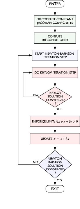
The BiCGSTAB iteration (Kelley, 1995; Saad, 2003) is implemented exactly as described in Barrett, et al. (1994). The iterative convergence of this method is hastened, or enabled, through the use of preconditioners (Chen, 2005). The particular preconditioning strategy that we employ is a 2-D extension of the sparse approximate inverse approach used for 1-D multigroup flux-limited diffusion problems (Swesty, Smolarski, & Saylor, 2004).
This iterative Newton-BiCGSTAB approach approach has several distinct advantages. First, the matrix corresponding to the Jacobian need not be computed and stored; instead, the Jacobian can be applied in operator form. Second, the knowledge of effective preconditioners from the linear flux-limited diffusion equation can be exploited to accelerate iterative convergence. Third, the method, including preconditioning, is easily parallelizable.
One minor deviation from standard Newton-Krylov iteration that we employ is the enforcement of positivity during the nonlinear iteration step. In Figure 29, we indicate this by the red box prior to the solution update. During this step, the Newton step for a particular variable is limited if it would result in a negative value for the energy density.
The stopping criterion for the Newton iteration is
| (H43) |
where the solution tolerance, , is chosen to be some value between and . In equation (H43), is the th estimate of the unknown vector is given by
| (H44) |
The stopping criterion for the Krylov iteration (BiCGSTAB) is based on the norm of the linear system residual , and is given by
| (H45) |
where is the right-hand-side of the linearized system of equations on each Newton iteration. We typically choose , based on extensive numerical trials, to yield an inexact-Newton method.
Appendix I Discretization of Energy and Lepton Exchange Equations
In the radiation-transport equations in Appendix H, collisional processes that change lepton number and/or energy of the components of the radiation field are included in the terms and in equations (H1) and (H2) respectively. Since these terms depend on the radiation energy densities and , once equations (H1) and (H2) have been solved, the amount of energy and lepton (if any) exchange is thus determined. Once the values of and are known, equations (35) and (40) can then be solved to accomplish steps , , and of Figure 3.
The right-hand side of equation (35) gives the total amount of lepton number exchange with a given flavor of radiation in terms of an integral over the spectrum:
| (I1) |
The leading superscript on quantities in equation (I1) is used to indicate radiation of the electron neutrino flavor (muon and tauon type neutrinos do not contribute to lepton number exchange since they are only produced in particle-antiparticle pairs). The first term in the integrand of equation (I1) gives the lepton number exchange between matter and radiation particles while the second term gives the lepton number exchange with antiparticles (if they are present). The minus sign in the second term reflects the negative quantum number assigned to the antiparticles.
In our discretization of equation (35), we replace the integral with a midpoint-rule summation and the time derivative with a forward difference to get
| (I2) |
which is the discretization of equation (35). Once the new value of the electron number density is known, the new electron fraction can be computed trivially as
| (I3) |
The solution of the energy exchange equation (eq. [40]) is similar to the solution of equation (35), but involves several additional steps. Although lepton number exchange only takes place for neutrinos of the electron flavor, the exchange of energy takes place for all flavors. The right-hand-side of equation (40) is given by
| (I4) |
where the leading superscript is used to indicate the flavor of the radiation-species (in the case of neutrinos equals , or ). Equation (40) thus becomes
| (I5) |
The concept of operator splitting can be applied to equation (I5), so we can solve separate equations of the form
| (I6) |
for each radiation species. These operator split sub-equations are each solved immediately after the solution of the radiation diffusion equation for the corresponding radiation flavor. In the case of electron type neutrinos in substep (box of Figure 3), equation (I6) is solved after equation (I2) is solved. Equation (I6) is solved for muon neutrinos in substep and for tauon neutrinos in substep .
The discretization of equation (I6) proceeds almost identically to the discretization of equation (I1). In substep the discretized equation solved to account for energy exchange with electron neutrinos is
| (I7) |
In substep the discretized equation solved to account for energy exchange with muon neutrinos is
| (I8) |
In substep the discretized equation solved to account for energy exchange with tauon neutrinos is
| (I9) |
In each of substeps , , and , it is necessary, after the new value of is obtained, to use the equation of state to obtain new values of the temperature and the pressure corresponding to the updated internal energy density and, in the case of substep , the new updated electron fraction. This is performed by inverting the EOS to find the temperature corresponding to the new energy density via a combination of Newton-Raphson and bisection methods for nonlinear equations.
In substep the new temperature is found by iteratively solving
| (I10) |
for the new temperature, based on the updated values of and . In the case of substep the equation solved for the new temperature is
| (I11) |
while in substep the equation solved is
| (I12) |
In each case, once the new temperature is known, the pressure is determined by the equation of state. The computational cost of the equation of state computations needed to solve iteratively equations (I10)-(I12) is negligible compared to the computational effort involved in solving the nonlinear systems corresponding to the radiation diffusion equations.
Appendix J Discretization of the Gas-Momentum Radiation Equation
In this appendix we describe the solution of equation (45). Following the update to gas momentum from the matter contribution, as described in Appendix F, we next update the gas momentum to account for radiation-matter interaction. This update corresponds to the solution of the term in equation (41),
| (J1) |
For radiation transport algorithms that have a non-zero radiation-matter momentum exchange, this step of the algorithm can also be used to solve for the term in equation (41). In such a case, the right-hand side of equation (J1) will have an additional term . As previously stated in §2, we assume . (However, see §2.4 for a discussion of radiation-transport algorithms and non-zero value of .)
To evaluate , we use Stone & Norman (1992a), equations (130)–(132). Note that several terms of these equations in Stone & Norman (1992a) have sign errors. Specifically, the term in their equation (130) and the term in their equation (131) both have the incorrect signs. Fortunately, these errors are irrelevant since the choice of the and for the coordinate systems under consideration makes these terms vanish. In writing the following expressions, we have omitted terms in the divergence that are always zero in our implementation. These include all terms in , terms proportional to zero-valued tensor elements , , terms proportional to derivatives of the constant function , and terms containing and , which are zero by definition. The remaining non-zero terms give
| (J2) | |||||
| (J3) | |||||
| (J4) |
The quantity represents the radiation pressure tensor containing contributions from the complete spectrum of radiation. Hence,
| (J5) |
where the sum over represents contributions from all species of radiation. The added term in parentheses indicates the possible presence of a distinct antiparticle that is also evolved. Remembering the definition of (see eq. [14]), this expands in terms of the Eddington tensor to give
| (J6) |
where, once again, the possible presence of an antiparticle is indicated in parentheses.
Expressing equation (J1) in differenced form (remembering that the density is constant over this step in the operator splitting and emerges from the time derivative), we have the following, where here, the possible antiparticle has been suppressed to make the equations readable, and the radiation-energy spectra have been discretized using index . This update corresponds to substep (see §3.4):
| (J7) | |||||
and
| (J8) | |||||
In this two-dimensional formulation, at all times. The summations run over energy index and species index . These expressions are evaluated over the entire spatial domain, i.e., for each index and . To include the effects of antiparticles in equations (J7) and (J8), the following substitution should be made in equations (J7) and (J8) for each instance of the expression to the left of the arrow:
| (J9) | |||||
Appendix K Implementation of Explicit Boundary Conditions
In this appendix we discuss the formulation and implementation of boundary conditions for the equations that are solved explicitly. Boundary conditions for the implicitly solved radiation-diffusion equations are discussed in Appendix H.
To permit solution of a wide range of problems, we have implemented multiple options for boundary conditions into V2D. In this appendix, we describe four such options: (i) flat, (ii) periodic, (iii) reflecting, and (iv) flux conserving. V2D makes no requirement that the same option be chosen in each direction or at each of the two boundaries in a given direction—in many problems, it is common for them to be different.
As shown in Figures 30 and 31, V2D is structured to use boundaries that are centered on the integer mesh, i.e., boundary interfaces lie on cell faces, not cell centers. In this appendix, for each option listed above, we present the necessary boundary-value assignments for both scalar and vector quantities. Since our differencing scheme uses values no farther from the point of interest than that of next-to-nearest neighbor, we need carry no more than two boundary cells.
In what follows, we describe the application of boundary conditions only in the direction. Application of the same sets of conditions in the direction is straightforward, as long as one remembers that components of vectors normal and tangential to the boundary interface are swapped.
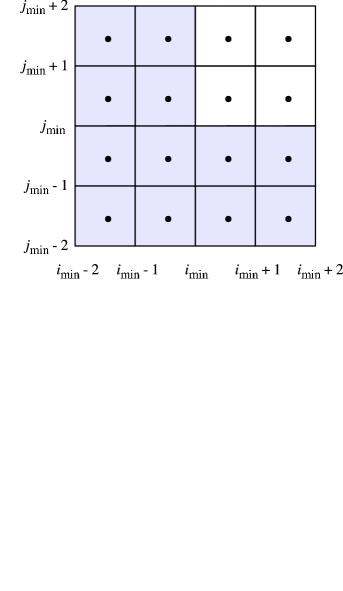
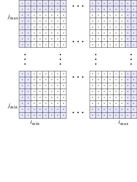
1. Flat Boundary Conditions. To implement flat boundary conditions in the direction, we apply the following procedure: First, for any scalar quantity , at the left-hand boundary, we set the values at the two left-hand boundary zones to the value at the first physical zone:
| (K1) |
This applies to all values of the index , which is also the case for all such equations in this appendix. Similarly, to implement flat conditions at the right-hand boundary, we set the scalar values of the two right-hand boundary zones to have the value of the last physical zone:
| (K2) |
For any vector quantity , the procedure is analogous. In the direction, for the component of vector , we use at left-hand boundary,
| (K3) |
where we note that is undefined. At the right-hand boundary we have
| (K4) |
We also need to specify how behaves at the both right- and left-hand boundaries. At the left-hand boundary,
| (K5) |
and, at the right,
| (K6) |
2. Periodic Boundary Conditions. Next, we apply periodic boundary conditions in the direction. For a scalar, we have at the left-hand boundary,
| (K7) |
| (K8) |
while at the right,
| (K9) |
| (K10) |
For vectors, the procedure is again analogous. In the direction, for at the left-hand boundary,
| (K11) |
| (K12) |
and at the right,
| (K13) |
| (K14) |
For at the left-hand boundary,
| (K15) |
| (K16) |
and at the right,
| (K17) |
| (K18) |
3. Reflecting Boundary Conditions. For scalars, applying reflecting boundary conditions in the direction, at the left boundary gives
| (K19) |
| (K20) |
and at the right-hand boundary,
| (K21) |
| (K22) |
For vector quantities, reflection symmetry requires that the normal component of a vector vanish at planes of symmetry, Thus, for reflecting boundary conditions in the direction, we have the following at the left-hand boundary for normal component, :
| (K23) |
| (K24) |
Similarly, at the right-hand boundary, we have
| (K25) |
| (K26) |
Since the tangential vector component, , is not defined at the planes of symmetry, we do not have to apply a zero-value requirement at boundaries. Hence, boundary values are reflected in the same way as scalars. At the left-hand boundary,
| (K27) |
| (K28) |
while at the right,
| (K29) |
| (K30) |
4. Flux-Conserving Boundary Conditions. This option is especially useful for problems with spherical geometry, when applied to the radial coordinate. Rather than keeping a physical quantity (such as density) constant across the boundary, this option allows flux of a physical quantity (such as mass flux) to be kept constant. At the outer boundary, a constant flux of is maintained when
| (K31) |
| (K32) |
If the same condition is desired at an inner boundary, for a problem where the computational grid does not extend all the way to , we have
| (K33) |
| (K34) |
Finally, it should be noted that the spatial boundary conditions we have just outlined are also applied to each spectral component of radiation quantities. Additionally, with spectral quantities, there is an another dimension for which boundary conditions must be applied—the energy dimension. In V2D, we always apply energy-space boundary conditions that prevent both inflow below the lowest group (the lower boundary is typically at zero anyway) and outflow beyond the highest group. In the case of the latter, we always carry a sufficient number of groups such that radiation occupancy in the higher groups is always small. Thus, it is largely irrelevant how we treat this upper boundary.
Appendix L Enforcing the Pauli Exclusion Principal for Neutrinos
As we discuss in §2.3, it is necessary to enforce the Pauli exclusion principle for neutrinos. Neither of the operator split portions of equation (6), the radiation diffusion equation (H1) and the neutrino advection equation (48), guarantee that the neutrino occupancy of a given energy state will remain less than unity. This reflects the fact that equation (6) is semiclassical in the sense that only the collision integral is treated in a quantum-mechanical fashion. Therefore, we must enforce the Pauli exclusion principle as a separate step in our algorithm. Other authors (Bruenn, 1985; Mezzacappa & Bruenn, 1993b) have adopted similar strategies.
The Pauli exclusion principle requires that the constraint (30) be satisfied. In general, when a numerical solution of equations (H1) or (48) are obtained, the newly calculated value of the neutrino radiation energy density may not satisfy this constraint. As neutrinos are produced during the collapse of a stellar core, the lower energy states in the center of the core become fully populated. The continued hydrodynamic compression of neutrinos within a spatial zone, as described by equation (H1) or (48), can result in occupation numbers greater than unity in a given group. In our finite difference notation, the Pauli constraint corresponds to
| (L1) |
where 9.4523 for both photons and neutrinos (for which ).
In order to counter this unphysical effect, we examine the radiation energy densities each time equation (H1) or (48) is solved. If the values of the radiation energy density in a specific group exceeds , the excess neutrinos are removed from that group and placed in the next highest energy group or groups where phase space is available. After this process is completed for all groups, the matter internal energy is corrected to account for any change in the total (integrated over the spectrum) neutrino energy density. A new temperature and pressure are then computed for the zone.
This enforcement algorithm is applied as the final operation in all substeps corresponding to the red boxes in Figure 3.
References
- Arakawa (1966) Arakawa, A. 1966, J. Comp. Phys., 1, 119 (reprinted in 1997, J. Comp. Phys., 135, 103)
- Barrett, et al. (1994) Barrett, R., et al. 1994, Templates for the Solution of Linear Systems: Building Blocks for Iterative Methods (Philadelphia: SIAM)
- Beaudet, Petrosian, & Salpeter (1967) Beaudet, G., Petrosian, V., & Salpeter, E. E. 1967, ApJ, 150, 979.
- Bludman (1977) Bludman, S. A. in Proc. Internat. Neutrino Conf., ed. G. Faissner at el. (BraunSchweig: Fedr. Vieweg), p. 633
- Bowers & Wilson (1982) Bowers, R. L., & Wilson, J. R. 1982, ApJS, 50, 115
- Bowers & Wilson (1991) Bowers, R. L., & Wilson, J. R. 1991, Numerical Modeling in Applied Physics and Astrophysics (Boston: Jones and Bartlett Publishers)
- Bruenn (1985) Bruenn, S. W. 1985, ApJS, 58, 771
- Buchler (1983) Buchler, J.-P. 1983, J. Quant. Spec. Rad. Transf., 30, 395
- Buras et al. (2006) Buras, R., Rampp. M., Janka, H.-Th., & Kifonidis, K. 2006, A&A, 447, 1049
- Butkov (1968) Butkov, E., 1968, Mathematical Physics, (Reading, MA, USA: Addison-Wesley Publishing Company)
- Calder et al. (2002) Calder. A. 2002, ApJS, 143, 201
- Calder et al. (2004) Calder. A. 2004, Comput. Sci. Eng., September 2004, 10
- Castor (2004) Castor, J. I. 2004, Radiation Hydrodynamics, (Cambridge: Cambridge University Press)
- Cernohorsky, van den Horn, & Cooperstein (1989) Cernohorsky, J., van den Horn, L. J. & Cooperstein, J. 1989, JQSRT, 42, 603
- Cernohorsky, & van den Horn (1990) Cernohorsky, J., & van den Horn, L. J. 1990, JQSRT, 43, 33
- Cernohorsky & Bludman (1994) Cernohorsky, J. & Bludman, S. A. 1994, ApJ, 433, 205
- Chandrasekhar (1967) Chandrasekhar, S. 1967, An Introduction to the Study of Stellar Structure, (New York: Dover Publications)
- Chen (2005) Chen, K. 2005, Matrix Preconditioning Techniques and Applications (Cambridge: Cambridge University Press)
- Colella & Glaz (1985) Colella, P., & Glaz, H. M. 1985, J. Comput. Phys., 59, 264
- Colella & Woodward (1984) Colella, P., & Woodward, P. R. 1984, J. Comput. Phys., 54, 174
- Courant & Friedrichs (1976) Courant, R., & Friedrichs, K. O. 1976, Supersonic Flow and Shock Waves (New York: Springer)
- Crank (1980) Crank, J. 1980, The Mathematics of Diffusion. 2nd ed. (Oxford: Oxford University Press)
- Dutta et al. (2004) Dutta, S. I., Ratković, S., Prakash, M. 2004, Phys. Rev. D, 69, 023005
- Fryxell et al. (2000) Fryxell, B., Olson, K., Ricker, P., Timmes, F. X., Zingale, M., Lamb, D. Q., MacNeice, P., Rosner, R., Truran, J. W., & Tufo, H., 2000, ApJS, 131, 273
- Fuller (1982) Fuller, G. M. 1982, ApJ, 252, 741
- Fuller et al. (1982) Fuller, G. M., Fowler, W. A., & Newman, M. J. 1982, ApJ, 252, 715
- Fuller et al. (1985) Fuller, G. M., Fowler, W. A., & Newman, M. J. 1985, ApJ, 293, 1
- Gradshteyn & Ryzhik (1994) Gradshteyn, I. S. & Ryzhik, I. M. 1994, Table of Integrals, Series, and Products (San Diego: Academic Press)
- Gropp et al. (1999a) Gropp, W., Lusk, E., & Skjellum, A. 1999, Using MPI, Portable Parallel Programming with the Message-Passing Interface, 2nd ed. (Cambridge, MA, USA: The MIT Press)
- Gropp et al. (1999b) Gropp, W., Lusk, E., & Thakur, R. 1999, Using MPI-2, Advanced Features of the Message-Passing Interface (Cambridge, MA, USA: The MIT Press)
- Gudunov (1959) Gudunov, S. K. 1959, Matematicheskii Sbornik, 47, 271
- Hawley et al. (1984a) Hawley, J. F., Smarr, L. L., & Wilson, J. R. 1984a, ApJ, 277, 296
- Hawley et al. (1984b) Hawley, J. F., Smarr, L. L., & Wilson, J. R. 1984b, ApJS, 55, 211
- Hayes & Norman (2003) Hayes, J. C., and Norman, M. L. 2003, ApJS, 147, 197
- Hayes et al. (2005) Hayes, J. C., Norman, M. L., Fiedler, R. A., Bordner, J. O., Li, P. S., Clark, S. E., ud-Doula, A., & MacLow, M.-M. 2005, preprint (astro-ph/0511545)
- Hix et al. (2003) Hix, W. R., Messer, O. E. B., Mezzacappa, A., Liebendörfer, M., Sampaio, J. M., Langanke, K., Dean, D. J., Martínez-Pinedo, G., 2003, Phys. Rev. Lett. 91, 201102
- Hix et al. (2005) Hix, W. R., Messer, O. E. B., Mezzacappa, A., Sampaio, J. M., Langanke, K., Martínez-Pinedo, G., Liebendörfer, M., Dean, D. J., 2005, Nucl. Phys. A 758, 31c
- Hunsdorfer & Verwer (2003) Hunsdorfer, W., Verwer, J. G. 2003, Numerical Solutions of Time-Dependent Advection-Diffusion-Reaction Equations. (New York: Springer)
- Janka (1991) Janka, H.-T. 1991, Dissertation, Technische Universität München
- Janka (1992) Janka, H.-T. 1992, A&A, 256, 452
- Janka et al. (1992) Janka, H.-T., Dagni, R., & van den Horn, L. J. 1992, A&A, 265, 345
- Kelley (1995) Kelley, C. T. 1995, Iterative Methods for Linear and Nonlinear Equations, (Philadelphia: SIAM)
- Kelley (2003) Kelley, C. T. 2003, Solving Nonlinear Equations with Newton’s Method, (Philadelphia: SIAM)
- Knupp & Salari (2002) Knupp, P. & Salari, K. 2002, Verification of Computer Codes in Computational Science and Engineering, (Kansas City: Chapman & Hall/CRC)
- Lamb (1995) Lamb, G. L.,Jr. 1995, Introductory Applications of Partial Differential Equations (New York: Wiley)
- Landau & Lifshitz (1959) Landau, L. D., & Lifshitz, E. M. 1959, Fluid Mechanics (Oxford: Pergamon Press)
- Langanke et al. (2003) Langanke, K., Martínez-Pinedo, G., Sampaio, J. M., Dean, D. J., Hix, W. R., Messer, O. E. B., Mezzacappa, A., Liebendörfer, M., Janka, H.-Th., & Rampp, M. 2003, Phys. Rev. Lett. 90, 241102
- Lattimer & Swesty (1991) Lattimer, J. M., & Swesty, F. D. 1991, Nucl. Phys. A, 535, 331
- Levermore (1984) Levermore, C. D. 1984, ApJ, 31, 149
- Levermore & Pomraning (1981) Levermore, C. D., & Pomraning, G. C. 1981, ApJ, 248, 321
- Liebendörfer et al. (2001) Liebendörfer, M., Mezzacappa, A., & Thielemann, F.-K. 2001, Phys Rev D, 63, 104003
- Liebendörfer et al. (2004) Liebendörfer, M., Messer, E. B., Bruenn, S. W., Cardall, C. Y. & Thielemann, F.-K. 2004, ApJS, 150, 263
- Livne et al. (2004) Livne, E., Burrows, A.,Walder, R., Lichtenstadt, I., & Thompson, T. A. 2004, Ap.J., 609, 277
- Lund (1983) Lund, C. M., 1985, in Numerical Astrophyics, ed. J. Centrella, J. M. LeBlanc, & R. Bowers, (Boston: Jones & Bartlett) 498
- Menikoff & Plohr (1989) Menikoff, R., & Plohr, B. J. 1989, Rev. Mod. Phys., 61, 75
- Mezzacappa & Bruenn (1993a) Mezzacappa, A., & Bruenn, S. W. 1993a, ApJ, 405, 637
- Mezzacappa & Bruenn (1993b) Mezzacappa, A., & Bruenn, S. W. 1993b, ApJ, 405, 669
- Mezzacappa & Bruenn (1993c) Mezzacappa, A., & Bruenn, S. W. 1993c, ApJ, 410, 740
- Mihalas & Mihalas (1983) Mihalas, D., & Mihalas, B. W. 1983, ApJ, 273, 355
- Mihalas & Mihalas (1984) Mihalas, D., & Mihalas, B. W. 1984, Foundations of Radiation Hydrodynamics (New York: Oxford University Press)
- Miller, Wilson, & Mayle (1993) Miller, D. S., Wilson, J. R. & Mayle, R. W. 1993, ApJ, 415, 278
- Minerbo (1978) Minerbo, G. N. 1978, JQSRT, 20, 451
- Mönchmeyer & Müller (1989) Mönchmeyer, R., & Müller, E. 1989, Astron. Astrophys., 217, 351
- Myra et al. (1987) Myra, E. S., Bludman, S. A., Hoffman, Y., Lichtenstadt, I., Sack, N., & Van Riper, K. A. 1987, ApJ, 318, 744
- Noh (1987) Noh,W. F., 1987, J. Comp. Phys. 72, 78
- Norman et al. (1980) Norman, M. L., Wilson, J. R., & Barton, R. 1980, ApJ, 239, 968
- Oran & Boris (2001) Oran, E. S., & Boris, J. P. 2001, Numerical Simulation of Reactive Flow, (Cambridge: Cambridge University Press)
- Pen (1998) Pen, U.-L., 1998, ApJS, 115, 19
- Pomraning (1981) Pomraning, G. C., 1981, JQSRT, 26, 385
- Pomraning (2005) Pomraning, G. C. 2005, The Equations of Radiation Hydrodynamics, (Mineola: Dover Publications Inc)
- Post & Votta (2005) Post, D. & Votta, L. 2005, Phys. Today, January, 35
- Ratković et al. (2003) Ratković, S., Dutta, S. I., Prakash, M. 2003, Phys. Rev. D, 67, 123002
- Richtmyer & Morton (1967) Richtmyer, R. D., & Morton, K. W., 1967, Difference Methods for Initial-Value Problems, 2nd. Ed. (New York: John Wiley & Sons)
- Riley, Hobson, & Bence (1998) Riley, K. F., Hobson, M. P., & Bence, S. J. 1998, Mathematical Methods for Physics and Engineering, (Cambridge: Cambridge University Press)
- Roache (1998) Roache, P. J., 1998, Verification and Validation in Computational Science and Engineering, (Albequerque: Hermosa)
- Saad (2003) Saad, Y. 2003, Iterative Methods for Sparse Linear Systems. (SIAM: Philadelphia)
- Schinder & Shapiro (1982) Schinder, P. J. & Shapiro, S. L. 1982, ApJS, 50, 23
- Schinder et al. (1987) Schinder, P. J, Schramm, D. N., Wiita, P. J., Margolis, S. H, Tubbs, D. L. 1987, ApJ, 313, 531
- Schinder (1988) Schinder, P. J. 1988, Phys. Rev., D38, 1637
- Schinder, Bludman, & Piran (1988) Schinder, P. J., Bludman, S. A. & Piran, T. 1988, Phys. Rev., D37, 2722
- Schinder & Bludman (1989) Schinder, P. J. & Bludman, S. A. 1989, ApJ, 346, 350
- Sedov (1959) Sedov, L. I. 1959, Similarity and Dimensional Methods in Mechanics, trans. M. Friedman (New York: Academic Press)
- Selby (1972) Selby, S. M., Ed. 1972, Standard Mathematical Tables (Cleveland: Chem. Ruuber Co.)
- Smit, van den Horn, & Bludman (2000) Smit, J. H., van den Horn, L. J. & Bludman, S. A. 2000, A&A, 356, 559
- Sod (1978) Sod, G. A., 1978, J. Comput. Phys., 23, 276
- Stone & Norman (1992a) Stone, J. M., & Norman, M. L. 1992, ApJS, 80, 753
- Stone & Norman (1992b) Stone, J. M., & Norman, M. L. 1992, ApJS, 80, 791
- Stone, Mihalas, & Norman (1992) Stone, J. M., Mihalas, D., & Norman, M. L. 1992, ApJS, 80, 819
- Swesty (1995) Swesty, F. D. 1995, ApJ, 445, 811
- Swesty (1996) Swesty, F. D. 1996, J. Comp. Phys, 127, 118
- Swesty (2006) Swesty, F. D. 2006, in Computational Methods in Transport, Granlibakken 2004, ed. F. Graziani (Berlin: Springer 2006) 469
- Swesty & Myra (2005a) Swesty, F. D., & Myra, E. S. 2005, in SciDAC 2005, Scientific Discovery through Advanced Computing; Journal of Physics: Conference Series, 16, 380
- Swesty, Smolarski, & Saylor (2004) Swesty, F. D., Smolarski, D. C., & Saylor, P. E. 2004, ApJS, 153, 369
- Taylor (1950) Taylor, G. 1950, Proc. Roy. Soc. Lon., Ser. A, 201, 159
- Turner & Stone (2001) Turner, N. J., & Stone, J. M. 2001, ApJS, 135, 95
- Tscharnuter and Winkler (1979) Tscharnuter, W.-M., and Winker, K.-H. 1979, Comput. Phys. Comm., 18, 171
- van Leer (1977) van Leer, B. 1977, J. Comput. Phys., 23, 276
- Woodward (1986) Woodward, P. R., 1986, in Astrophysical Radiation Hydrodynamics, ed. K.-H. Winkler & M. L. Norman (Dordrecht: Reidel) 245
- Yueh & Buchler (1976) Yueh, W. R., & Buchler, J. R. 1976, Ap. Space Sci., 41, 221
- Yueh & Buchler (1977) Yueh, W. R., & Buchler, J. R. 1977, ApJ, 217, 565
- Zel’dovich & Razier (1967) Zel’dovich, Ya. B., & Razier, Yu. P. 1967, Physics of Shock Waves and High-Temperature Hydrodynamic Phenomena (New York: Academic Press)