Density-functional-theory calculations of matter in strong magnetic fields. II. Infinite chains and condensed matter

Abstract

We present calculations of the electronic structure of one-dimensional infinite chains and three-dimensional condensed matter in strong magnetic fields ranging from $B=10^{12}$ G to $2\times 10^{15}$ G, appropriate for observed magnetic neutron stars. At these field strengths, the magnetic forces on the electrons dominate over the Coulomb forces, and to a good approximation the electrons are confined to the ground Landau level. Our calculations are based on the density functional theory, and use a local magnetic exchange-correlation function appropriate in the strong field regime. The band structures of electrons in different Landau orbitals are computed self-consistently. Numerical results of the ground-state energies and electron work functions are given for one-dimensional chains H_∞, He_∞, C_∞, and Fe_∞. Fitting formulae for the $B$-dependence of the energies are also provided. For all the field strengths considered in this paper, hydrogen, helium, and carbon chains are found to be bound relative to individual atoms (although for $B$ less than a few $\times 10^{12}$ G, carbon infinite chains are very weakly bound relative to individual atoms). Iron chains are significantly bound for $B\gtrsim 10^{14}$ G and are weakly bound if at all at $B\lesssim 10^{13}$ G. We also study the cohesive property of three-dimensional condensed matter of H, He, C, and Fe at zero pressure, constructed from interacting chains in a body-centered tetragonal lattice. Such three-dimensional condensed matter is found to be bound relative to individual atoms, with the cohesive energy increasing rapidly with increasing $B$.

I Introduction

Young neutron stars (ages $\lesssim 10^{7}$ years) are observed to have surface magnetic fields in the range of $10^{11}$-$10^{15}$ G (meszaros92, ; reisenegger05, ; woods05, ; harding06, ), far beyond the reach of terrestrial laboratories (wagner04, ). It is well known that the properties of matter can be drastically modified by such strong magnetic fields. The natural atomic unit for the magnetic field strength, $B_{0}$, is set by equating the electron cyclotron energy $\hbar\omega_{Be}=\hbar(eB/m_{e}c)=11.577\,B_{12}$ keV, where $B_{12}=B/(10^{12}~{}{\rm G})$, to the characteristic atomic energy $e^{2}/a_{0}=2\times 13.6$ eV (where $a_{0}$ is the Bohr radius):

$$B_{0}={m_{e}^{2}e^{3}c\over\hbar^{3}}=2.3505\times 10^{9}\,{\rm G}.$$ (1)

For $b=B/B_{0}\gtrsim 1$, the usual perturbative treatment of the magnetic effects on matter (e.g., Zeeman splitting of atomic energy levels) does not apply. Instead, in the transverse direction (perpendicular to the field) the Coulomb forces act as a perturbation to the magnetic forces, and the electrons in an atom settle into the ground Landau level. Because of the extreme confinement of the electrons in the transverse direction, the Coulomb force becomes much more effective in binding the electrons along the magnetic field direction. The atom attains a cylindrical structure. Moreover, it is possible for these elongated atoms to form molecular chains by covalent bonding along the field direction. Interactions between the linear chains can then lead to the formation of three-dimensional condensed matter (ruderman74, ; ruder94, ; Lai, 2001).

This paper is the second in a series where we present calculations of matter in strong magnetic fields using density functional theory. In Medin and Lai (2006) (hereafter paper I), we studied various atoms and molecules in magnetic fields ranging from $10^{12}$ G to $2\times 10^{15}$ G for H, He, C, and Fe, representative of the most likely neutron star surface compositions. Numerical results and fitting formulae of the ground-state energies were given for H_N (up to $N=10$), He_N (up to $N=8$), C_N (up to $N=5$), and Fe_N (up to $N=3$), as well as for various ionized atoms. It was found that as $B$ increases, molecules become increasingly more bound relative to individual atoms, and that the binding energy per atom in a molecule, $|E_{N}|/N$, generally increases and approaches a constant value with increasing $N$. In this paper, we present density-functional-theory calculations of infinite chains of H, He, C, and Fe. Our goal is to obtain the cohesive energy of such one-dimensional (1D) condensed matter relative to individual atoms for a wide range of field strengths. We also carry out approximate calculations of the relative binding energy between 1D chains and three-dimensional (3D) condensed matter at zero pressure.

The cohesive property of matter in strong magnetic fields is a fundamental quantity characterizing magnetized neutron star surface layers, which play a key role in many neutron star processes and observed phenomena. The cohesive energy refers to the energy required to pull an atom out of the bulk condensed matter at zero pressure. Theoretical models of pulsar and magnetar magnetospheres depend on the cohesive properties of the surface matter in strong magnetic fields (ruderman75, ; arons79, ; usov96, ; harding98, ; beloborodov06, ; gil03, ). For example, depending on the cohesive energy of the surface matter, an acceleration zone (“polar gap”) above the polar cap of a pulsar may or may not form, and this will affect pulsar radio emission and other high-energy emission processes. Also, while a hot or warm neutron star most certainly has a gaseous atmosphere that mediates its thermal emission, condensation of the stellar surface may occur at sufficiently low temperatures (lai97, ; Lai, 2001). For example, radiation from a bare condensed surface (with no atmosphere above it) has been invoked to explain the nearly perfect blackbody emission spectra observed in some nearby isolated neutron stars (burwitz03, ; mori03, ; vanadelsberg05, ; turolla04, ; perez06, ). However, whether surface condensation actually occurs depends on the cohesive energy of the surface matter.

There have been few quantitative studies of infinite chains and zero-pressure condensed matter in strong magnetic fields. Earlier variational calculations (flowers77, ; Müller, 1984) as well as calculations based on Thomas-Fermi type statistical models (Abrahams and Shapiro, 1991; fushiki92, ; lieb94a, ; lieb94b, ), while useful in establishing scaling relations and providing approximate energies of the atoms and the condensed matter, are not adequate for obtaining reliable energy differences (cohesive energies). Quantitative results for the energies of infinite chains of hydrogen molecules H_∞ in a wide range of field strengths ($B\gg B_{0}$) were presented in both Ref. (Lai et al., 1992) (using the Hartree-Fock method with the plane-wave approximation; see also Ref. (Lai, 2001) for some results of He_∞) and Ref. (Relovsky and Ruder, 1996) (using density functional theory). For heavier elements such as C and Fe, the cohesive energies of 1D chains have only been calculated at a few magnetic field strengths in the range of $B=10^{12}$-$10^{13}$ G, using Hartree-Fock models (Neuhauser et al., 1987) and density functional theory (Jones, 1985). There were discrepancies between the results of these works, and some (e.g., Ref. (Neuhauser et al., 1987)) adopted a crude treatment for the band structure (see Sec. III.3). An approximate calculation of 3D condensed matter based on density functional theory was presented in Ref. (Jones, 1986).

Our calculations of atoms and small molecules (paper I) and of infinite chains and condensed matter (this paper) are based on density functional theory (hohen64, ; kohn65, ; vignale87, ; vignale88, ; jones89, ). In the strong field regime where the electron spins are aligned with each other, the Hartree-Fock method is expected to be highly accurate (Neuhauser et al., 1987; schmelcher99, ). However, in dealing with systems with many electrons, it becomes increasingly impractical as the magnetic field increases, since more and more Landau orbitals (even though electrons remain in the ground Landau level) are occupied and keeping track of the direct and exchange interactions between electrons in various orbitals becomes computational rather tedious. Our density-functional calculations allow us to obtain the energies of atoms and small molecules and the energy of condensed matter using the same method, thus providing reliable cohesive energy values for condensed surfaces of magnetic neutron stars, a main goal of our study. Compared to previous density-functional theory calculations (Jones, 1985, 1986; kossl88, ; Relovsky and Ruder, 1996), we use an improved exchange-correlation function appropriate for highly magnetized electron gases, we calibrate our density-functional code with previous results (when available) based on other methods, and (for calculations of condensed matter) adopt a more accurate treatment of the band structure. Moreover, our calculations extend to the magnetar-like field regime ($B\sim 10^{15}$ G).

This paper is organized as follows. After briefly summarizing the approximate scaling relations for linear chains and condensed matter in strong magnetic fields in Sec. II, we describe our method and the basic equations in Sec. III. Numerical results (tables and fitting formulae) for linear chains are presented in Sec. IV. In Sec. V we describe our approximate calculation and results for the relative energy between 1D chain and 3D condensed matter. We conclude in Sec. VI. Some technical details are given in the appendix.

II Basic scaling relations for linear chains and 3D condensed matter in strong magnetic fields

The simplest model for the linear chain is to treat it as a uniform cylinder of electrons, with ions aligned along the magnetic field axis. The radius of the cylinder is $R$ and the length of a unit cell is $a$ (which is also the atomic spacing along the $z$ axis). The electrons lie in the ground Landau level, but can occupy different Landau orbitals with the radius of guiding center $\rho_{m}=(2m+1)^{1/2}\rho_{0}$, where $m=0,1,2,\ldots,m_{\rm max}$ and $\rho_{0}=(\hbar c/eB)^{1/2}=b^{-1/2}$ (in atomic units). The maximum Landau orbital number $m_{\rm max}$ is set by $\rho_{m_{\rm max}}=R$, giving $m_{\rm max}\simeq\pi R^{2}eB/(hc)=R^{2}b/2$ (this is the Landau degeneracy in area $\pi R^{2}$). For a uniform electron density $n=Z/(\pi R^{2}a)$, the Fermi wave number (along $z$) $k_{F}$ is determined from $n=bk_{F}/(2\pi^{2})$, and the kinetic energy of the electrons in a cell is $E_{k}=(Z/3)\varepsilon_{F}^{\prime}$, with $\varepsilon_{F}^{\prime}=k_{F}^{2}/2$ the Fermi kinetic energy. The total energy per atom (unit cell) in the chain can be written as (ruderman71, ; ruderman74, )

$$E_{\infty}={2\pi^{2}Z^{3}\over 3b^{2}R^{4}a^{2}}-{Z^{2}\over a}\left[\ln{2a\over R}-\left(\gamma-{5\over 8}\right)\right],$$ (2)

where $\gamma=0.5772\ldots$ is Euler’s constant. In Eq. (2), the first term is the electron kinetic energy $E_{k}$ and the second term is the (direct) Coulomb energy (the Madelung energy for the one-dimensional uniform lattice). Minimizing $E_{\infty}$ with respect to $R$ and $a$ gives

$$R=1.65\,Z^{1/5}b^{-2/5},\qquad a/R=2.14,$$

$$E_{\infty}=-0.354\,Z^{9/5}b^{2/5}.$$ (3)

Note that the energy (2) can be written as $E_{\infty}=-ZV_{0}+(Z/3)\varepsilon_{F}^{\prime}$, where $V_{0}$ is the depth of the potential well relative to the continuum. In equilibrium $E_{\infty}=-5E_{k}=-(5/3)Z\varepsilon_{F}^{\prime}$, and thus $V_{0}=2\varepsilon_{F}^{\prime}$. The Fermi level energy of the electrons in the chain relative to the continuum is then $\varepsilon_{F}=\varepsilon_{F}^{\prime}-V_{0}=-\varepsilon_{F}^{\prime}=3E_{\infty}/(5Z)$, i.e.,

$$\varepsilon_{F}(1D)=-0.212\,Z^{4/5}b^{2/5}\mbox{ a.u.}=-65.1\,Z^{4/5}B_{12}^{2/5}\mbox{ eV.}$$ (4)

Alternatively, if we identify the number of electrons in a cell, $N_{e}$, as an independent variable, we find $R=1.65\,(N_{e}^{2}/Z)^{1/5}b^{-2/5}$ and $E_{\infty}=-0.354\,(Z^{2}N_{e})^{3/5}b^{2/5}$. The chemical potential (which includes potential energy) of electrons in the chain is simply $\mu=\varepsilon_{F}=\partial E_{\infty}/\partial N_{e}$, in agreement with Eq. (4). The electron work function is $W=|\varepsilon_{F}|$.

A linear 1D chain naturally attracts neighboring chains through the quadrupole-quadrupole interaction. By placing parallel chains close together (with spacing of order $b^{-2/5}$), we obtain three-dimensional condensed matter (e.g., a body-centered tetragonal lattice) (ruderman71, ).

The binding energy of the 3D condensed matter at zero pressure can be estimated using the uniform electron gas model. Consider a Wigner-Seitz cell with radius $r_{i}=Z^{1/3}r_{s}$ ($r_{s}$ is the mean electron spacing); the mean number density of electrons is $n=Z/(4\pi r_{i}^{3}/3)$. When the Fermi energy $p_{F}^{2}/(2m_{e})$ is less than the electron cyclotron energy $\hbar\omega_{Be}$, or when the electron number density satisfies $n\leq n_{B}=(\sqrt{2}\pi^{2}\rho_{0}^{3})^{-1}=0.0716\,b^{3/2}$ (or $r_{i}\geq r_{iB}=1.49\,Z^{1/3}b^{-1/2}$), the electrons only occupy the ground Landau level. The energy per cell can be written

$$E_{s}(r_{i})={3\pi^{2}Z^{3}\over 8b^{2}r_{i}^{6}}-{0.9Z^{2}\over r_{i}},$$ (5)

where the first term is the kinetic energy and the second term is the Coulomb energy. For a zero-pressure condensed matter, we require $dE_{s}/dr_{i}=0$, and the equilibrium $r_{i}$ and energy are then given by

$$r_{i}\simeq 1.90\,Z^{1/5}b^{-2/5},$$ (6)

$$E_{s}\simeq-0.395\,Z^{9/5}b^{2/5}.$$ (7)

The corresponding zero-pressure condensation density is

$$\rho_{s}\simeq 561\,A\,Z^{-3/5}B_{12}^{6/5}\,{\rm g~{}cm}^{-3}.$$ (8)

The electron Fermi level energy is

$$\varepsilon_{F}(3D)=\frac{3}{5Z}E_{s}=-0.237\,Z^{4/5}b^{2/5}\mbox{ a.u.}=-72.7\,Z^{4/5}B_{12}^{2/5}\mbox{ eV.}$$ (9)

The uniform electron gas model can be improved by incorporating the Coulomb exchange energy and Thomas-Fermi correction due to nonuniformity of the electron gas (Lai, 2001; fushiki89, ).

Although the simple uniform electron gas model and its Thomas-Fermi type extensions give a reasonable estimate for the binding energy for the condensed state, they are not adequate for determining the cohesive property of the condensed matter. Also, as we shall see, Eq. (4) or Eq. (9) does not give a good scaling relation for the electron work function when detailed electron energy levels (bands) in the condensed matter are taken into account. The cohesive energy $Q_{s}=E_{a}-E_{s}$ is the difference between the atomic ground-state energy $E_{a}$ and the condensed matter energy per cell $E_{s}$. In principle, a three-dimensional electronic band structure calculation is needed to solve this problem. However, for sufficiently strong magnetic fields, such that $a_{0}/Z\gg\sqrt{2Z+1}\rho_{0}$ or $B_{12}\gg 100\,(Z/26)^{3}$, a linear 1D chain is expected to be strongly bound relative to individual atoms (i.e., the cohesive energy of the chain, $Q_{\infty}=E_{a}-E_{\infty}$, is significantly positive) (Lai, 2001). For such strong fields, the binding of 3D condensed matter results mainly from the covalent bond along the magnetic axis, rather than from chain-chain interactions; in another word, the energy difference $|\Delta E_{s}|=|E_{s}-E_{\infty}|$ is small compared to $Q_{\infty}$. In the magnetic field regime where $Q_{\infty}$ is small or even negative, chain-chain interactions are important in deciding whether 3D condensed matter is bound relative to individual atoms. In this paper we will concentrate on calculating $E_{\infty}$ and $Q_{\infty}$ for linear chains (Sec. III and Sec. IV). In Sec. V we shall quantify the magnitude of $\Delta E_{s}$ for different elements and field strengths.

III Density-functional-theory calculations of 1D chains: Methods and equations

Our calculations of 1D infinite chains are based on density functional theory, which is well established in the strong magnetic field regime ($B\gg B_{0}$) of interest here (vignale87, ; vignale88, ). Extensive comparisons of our density-functional-theory results for atoms and finite molecules with previous results (when available) based on different methods were given in paper I (Medin and Lai, 2006); such comparisons established the validity and calibrate the systematic error of our approach. As we discuss below, for infinite chains considered in the present paper, it is important to calculate the band structure of electrons (for different Landau orbitals) self-consistently, rather than using certain approximate ansätze as adopted in some previous works (Neuhauser et al., 1987).

III.1 Basic equations and concepts

Our calculations will be based on the “adiabatic approximation,” in which all electrons are assumed to lie in the ground Landau level. For elements with nuclear charge number $Z$, this is an excellent approximation for $b\gg Z^{2}$. Even under the more relaxed condition $b\gg Z^{4/3}$, this approximation is expected to yield a reasonable total energy and accurate results for the energy difference between different electronic systems (atoms and chains) (see paper I). Also, we use nonrelativisitc quantum mechanics in our calculations, even when $\hbar\omega_{Be}\gtrsim m_{e}c^{2}$ or $B\gtrsim B_{Q}=B_{0}/\alpha^{2}=4.414\times 10^{13}$ G. As discussed in paper I, this is accurate as long as the electrons stay in the ground Landau level.

In a 1D chain, the ions form a periodic lattice along the magnetic field axis. The number of cells (“atoms”) in the chain is $N\rightarrow\infty$ and the ions are equally spaced with lattice spacing $a$. In the adiabatic approximation, the one-electron wave function (“orbital”) can be separated into a transverse (perpendicular to the external magnetic field) component and a longitudinal (along the magnetic field) component:

$$\Psi_{m\nu k}(\mathbf{r})=\frac{1}{\sqrt{N}}W_{m}(\mathbf{r_{\perp}})f_{m\nu k}(z)\,.$$ (10)

Here $W_{m}$ is the ground-state Landau wave function (landau77, ) given by

$$W_{m}(\mathbf{r_{\perp}})=\frac{1}{\rho_{0}\sqrt{2\pi m!}}\left(\frac{\rho}{\sqrt{2}\rho_{0}}\right)^{m}\exp\left(\frac{-\rho^{2}}{4\rho_{0}^{2}}\right)\exp(-im\phi)\,,$$ (11)

which is normalized as $\int\!d^{2}{\bf r}_{\perp}|W_{m}|^{2}=1$. The longitudinal wave function $f_{m\nu k}$ must be solved numerically, and we choose to normalize it over a unit cell of the lattice:

$$\int_{-a/2}^{a/2}|f_{m\nu k}(z)|^{2}\,dz=1,$$ (12)

so that normalization of $\Psi_{m\nu k}$ is $\int\!d^{3}{\bf r}\,|\Psi_{m\nu k}|^{2}=1$ (here and henceforth, the general integral sign $\int\!d^{3}{\bf r}$ refers to integration over the whole chain, with $z$ from $-Na/2$ to $Na/2$). The index $\nu=0,1,2,\ldots$ labels the different bands of the electron (see below), rather than the number of nodes in the longitudinal wave function as in the atom or molecule case.

The quantum number $k$ is not present for atoms or finite molecules, but enters here because of the periodic nature of the electrons in the longitudinal direction. By Bloch’s theorem, the electrons satisfy the periodicity condition

$$f_{m\nu k}(z+a)=e^{ika}f_{m\nu k}(z)\,,$$ (13)

and $k$ is the Bloch wave number. Note that the longitudinal wave functions are periodic in $k$ with period $\Delta k=2\pi/a$; i.e., $f_{m\nu,k+K}(z)=f_{m\nu k}(z)$ with $K$ being any reciprocal vector (number, in one dimension) of the lattice, $K=2\pi n/a$ ($n$ is an integer). Because of this, to ensure that each wave function $f_{m\nu k}$ is unique, we restrict $k$ to the first Brillouin zone, $k\in[-\pi/a,\pi/a]$. The electrons fill each $(m\nu)$ band, with spacing $\Delta k=\pi/(Na)$, and thus the maximum number of electrons in a given band is $N$ (out of the total $ZN$ electrons in the chain). In another word, the number of electrons per unit cell in each ($m\nu$) band is $\sigma_{m\nu}\leq 1$ (see Sec. III.2).

The density distribution of electrons in the chain is given by

$$n(\mathbf{r})=\sum_{m\nu k}|\Psi_{m\nu k}(\mathbf{r})|^{2}=\frac{a}{2\pi}\sum_{m\nu}|W_{m}|^{2}(\rho)\int_{I_{m\nu}}dk\,|f_{m\nu k}(z)|^{2}\,,$$ (14)

where the sum/integral is over all electron states, each electron occupying an $(m\nu k)$ orbital. The notation $|W_{m}|^{2}(\rho)=|W_{m}(\mathbf{r}_{\perp})|^{2}$ is used here because $W_{m}$ is a function of $\rho$ and $\phi$ but $|W_{m}|^{2}$ is a function of $\rho$ only. The notation $\int_{I_{m\nu}}$ in the $k$ integral refers to the fact that the region of integration depends on the $(m\nu)$ level; we will discuss this interval and electron occupations in Sec. III.2. To simplify the appearance of the electron density expression, we define the function

$$\bar{f}_{m\nu}(z)=\sqrt{\frac{a}{2\pi}\int_{I_{m\nu}}dk\,|f_{m\nu k}(z)|^{2}}\,,$$ (15)

so that

$$n(\mathbf{r})=\sum_{m\nu}|W_{m}|^{2}(\rho)\bar{f}_{m\nu}^{\,2}(z)\,.$$ (16)

In an external magnetic field, the Hamiltonian of a free electron is

$$\hat{H}=\frac{1}{2m_{e}}\left(\mathbf{p}+\frac{e}{c}\mathbf{A}\right)^{2}+\frac{\hbar eB}{2m_{e}c}\sigma_{z}\,,$$ (17)

where $\mathbf{A}=\frac{1}{2}\mathbf{B}\times\mathbf{r}$ is the vector potential of the external magnetic field and $\sigma_{z}$ is the $z$-component Pauli spin matrix. For electrons in Landau levels, with their spins aligned parallel/antiparallel to the magnetic field, the Hamiltonian becomes

$$\hat{H}=\frac{\hat{p}_{z}^{2}}{2m_{e}}+\left(n_{L}+\frac{1}{2}\right)\hbar\omega_{Be}\pm\frac{1}{2}\hbar\omega_{Be}\,,$$ (18)

where $n_{L}=0,1,2,\ldots$ is the Landau level index; for electrons in the ground Landau level, with their spins aligned antiparallel to the magnetic field (so $n_{L}=0$ and $\sigma_{z}\rightarrow-1$),

$$\hat{H}=\frac{\hat{p}_{z}^{2}}{2m_{e}}\,.$$ (19)

The total Hamiltonian for the atom or molecule then becomes

$$\hat{H}=\sum_{i}\frac{\hat{p}_{z,i}^{2}}{2m_{e}}+V\,,$$ (20)

where the sum is over all electrons and $V$ is the total potential energy of the atom or molecule.

In the density functional formalism, the total energy per cell of the chain is expressed as a functional of the total electron density $n(\mathbf{r})$:

$$E[n]=E_{K}[n]+E_{eZ}[n]+E_{\rm dir}[n]+E_{\rm exc}[n]+E_{ZZ}[n]\,.$$ (21)

Here $E_{K}[n]$ is the kinetic energy of the system of non-interacting electrons, and $E_{eZ}$, $E_{\rm dir}$ and $E_{ZZ}$ are the electron-ion Coulomb energy, the direct electron-electron interaction energy and the ion-ion interaction energy, respectively:

$$E_{eZ}[n]=-\!\!\sum_{j=-N/2}^{N/2}Ze^{2}\int_{|z|<a/2}d\mathbf{r}\,\frac{n(\mathbf{r})}{|\mathbf{r}-\mathbf{z}_{j}|}\,,$$ (22)

$$E_{\rm dir}[n]=\frac{e^{2}}{2}\int\!\!\int_{|z|<a/2}d\mathbf{r}\,d\mathbf{r}^{\prime}\,\frac{n(\mathbf{r})n(\mathbf{r}^{\prime})}{|\mathbf{r}-\mathbf{r}^{\prime}|}\,,$$ (23)

$$E_{ZZ}[n]=\sum_{j=1}^{N/2}\frac{Z^{2}e^{2}}{ja}\,.$$ (24)

The location of the ions in the above equations is represented by the set $\{\mathbf{z}_{j}\}$, with

$${\bf z}_{j}=ja\hat{\mathbf{z}},\quad j=(-N/2),(-N/2+1),\ldots,0,\ldots,N/2.$$ (25)

The term $E_{\rm exc}$ represents the exchange-correlation energy. In the local approximation,

$$E_{\rm exc}[n]=\int_{|z|<a/2}\!d\mathbf{r}\,n(\mathbf{r})\,\varepsilon_{\rm exc}(n)\,,$$ (26)

where $\varepsilon_{\rm exc}(n)=\varepsilon_{\rm ex}(n)+\varepsilon_{\rm corr}(n)$ is the exchange and correlation energy per electron in a uniform electron gas of density $n$. For electrons in the ground Landau level, the (Hartree-Fock) exchange energy can be written as (danz71, )

$$\varepsilon_{\rm ex}(n)=-\pi e^{2}\rho_{0}^{2}nF(t)\,,$$ (27)

where the dimensionless function $F(t)$ is

$$F(t)=4\int_{0}^{\infty}\!\!\!dx\left[\tan^{-1}\left({1\over x}\right)-{x\over 2}\ln\left(1+{1\over x^{2}}\right)\right]e^{-4tx^{2}},$$ (28)

and

$$t=\left(\frac{n}{n_{B}}\right)^{2}=2\pi^{4}\rho_{0}^{6}n^{2},$$ (29)

[$n_{B}=(\sqrt{2}\pi^{2}\rho_{0}^{3})^{-1}$ is the density above which the higher Landau levels start to be filled in a uniform electron gas]. For small $t$, $F(t)$ can be expanded as (fushiki89, )

$$F(t)\simeq 3-\gamma-\ln 4t+\frac{2t}{3}\left(\frac{13}{6}-\gamma-\ln 4t\right)+\frac{8t^{2}}{15}\left(\frac{67}{30}-\gamma-\ln 4t\right)+{\cal O}(t^{3}\ln t),$$ (30)

where $\gamma=0.5772\ldots$ is Euler’s constant. We have found that the condition $t\ll 1$ is well satisfied everywhere for almost all infinite chains in our calculations. The notable exceptions are the carbon chains at $B=10^{12}$ G and the iron chains at $B\leq 10^{13}$ G, which have $t\lesssim 1$ near the center of each cell. These chains are expected to have higher $t$ values than the other chains in our calculations, as they have large $Z$ and low $B$ .

The correlation energy of uniform electron gas in strong magnetic fields has not be calculated in general, except in the regime $t\ll 1$ and Fermi wave number $k_{F}=2\pi^{2}\rho_{0}^{2}n\gg 1$ [or $n\gg(2\pi^{3}\rho_{0}^{2}a_{0})^{-1}$]. Skudlarski and Vignale (1993) use the random-phase approximation to find a numerical fit for the correlation energy in this regime (see also Ref. (stein98, )):

$$\varepsilon_{\rm corr}=-\frac{e^{2}}{\rho_{0}}\,[0.595(t/b)^{1/8}(1-1.009t^{1/8})]\,.$$ (31)

In the absence of an “exact” correlation energy density we employ this strong-field-limit expression. Fortunately, because we are concerned mostly with finding the energy difference between atoms and chains, the correlation energy term does not have to be exact. The presence or the form of the correlation term has a modest effect on the atomic and chain energies calculated but has very little effect on the energy difference between them (see paper I for more details on various forms of the correlation energy and comparisons).

Variation of the total energy with respect to the electron density, $\delta E[n]/\delta n=0$, leads to the Kohn-Sham equation:

$$\left[-\frac{\hbar^{2}}{2m_{e}}\nabla^{2}+V_{\rm eff}(\mathbf{r})\right]\Psi_{m\nu k}(\mathbf{r})=\varepsilon_{m\nu}(k)\Psi_{m\nu k}(\mathbf{r})\,,$$ (32)

where

$$V_{\rm eff}(\mathbf{r})=-\!\!\sum_{j=-N/2}^{N/2}\frac{Ze^{2}}{|\mathbf{r}-\mathbf{z}_{j}|}+e^{2}\int d\mathbf{r}^{\prime}\,\frac{n(\mathbf{r}^{\prime})}{|\mathbf{r}-\mathbf{r}^{\prime}|}+\mu_{\rm exc}(n),$$ (33)

with

$$\mu_{\rm exc}(n)=\frac{\partial(n\varepsilon_{\rm exc})}{\partial n}\,.$$ (34)

Averaging the Kohn-Sham equation over the transverse wave function yields a set of one-dimensional equations:

$$\left[-\frac{\hbar^{2}}{2m_{e}}\frac{d^{2}}{dz^{2}}+{\bar{V}}_{\rm eff}(z)\right]f_{m\nu k}(z)=\varepsilon_{m\nu}(k)f_{m\nu k}(z)\,.$$ (35)

where

$${\bar{V}}_{\rm eff}(z)=-Ze^{2}\!\sum_{j=-N/2}^{N/2}\int d\mathbf{r}_{\perp}\,\frac{|W_{m}|^{2}(\rho)}{|\mathbf{r}-\mathbf{z}_{j}|}+e^{2}\int\!\!\int d\mathbf{r}_{\perp}\,d\mathbf{r}^{\prime}\,\frac{|W_{m}|^{2}(\rho)\,n(\mathbf{r}^{\prime})}{|\mathbf{r}-\mathbf{r}^{\prime}|}$$

$$\qquad\qquad+\int d\mathbf{r}_{\perp}\,|W_{m}|^{2}(\rho)\,\mu_{\rm exc}(n).$$ (36)

This set of equations are solved self-consistently to find the eigenvalue $\varepsilon_{m\nu}(k)$ and the longitudinal wave function $f_{m\nu k}(z)$ for each orbital occupied by the electrons. Once these are known, the total energy per cell of the infinite chain can be calculated using

$$E_{\infty} = \frac{a}{2\pi}\sum_{m\nu}\int_{I_{m\nu}}dk\,\varepsilon_{m\nu}(k)-\frac{e^{2}}{2}\int\!\!\int_{|z|<a/2}d\mathbf{r}d\mathbf{r}^{\prime}\,\frac{n(\mathbf{r})n(\mathbf{r}^{\prime})}{|\mathbf{r}-\mathbf{r}^{\prime}|}$$ (37)

$$+\int_{|z|<a/2}d\mathbf{r}\,n(\mathbf{r})[\varepsilon_{\rm exc}(n)-\mu_{\rm exc}(n)]+\sum_{j=1}^{N/2}\frac{Z^{2}e^{2}}{ja}\,,$$

where the interval $I_{m\nu}$ is the same as in the electron density expression, Eq. (16).

Note that the electron-ion, direct electron-electron, and ion-ion interaction energy terms given above formally diverge for $N\rightarrow\infty$. These terms must be properly combined to yield a finite net potential energy. Note that for an electron in the “primary” unit cell ($-a/2\leq z\leq a/2$), the potential generated by a distant cell (centered at $z_{j}=ja$) can be well approximated by the quadrupole potential:

$$V_{Q}(\rho,z;ja)=\frac{3e^{2}}{2}\frac{Q_{zz}}{|ja|^{5}}\left(2z^{2}-\rho^{2}\right),$$ (38)

where $Q_{zz}$ is the quadrupole moment of a unit cell

$$Q_{zz}=\int_{|z|<a/2}d\mathbf{r}\,\left(2z^{2}-\rho^{2}\right)n(\rho,z)\,.$$ (39)

The Coulomb (quadrupole-quadrupole) energy between the primary cell and the distant cell is simply

$$E_{QQ}(ja)=\int_{|z|<a/2}d\mathbf{r}\,n({\bf r})\,V_{Q}(\rho,z;ja)=\frac{3e^{2}}{2}\frac{Q_{zz}^{2}}{|ja|^{5}}\,.$$ (40)

In our calculations, we treat distant cells with $|j|>N_{Q}$ using the quadrupole approximation, while treating the nearby cells ($|j|\leq N_{Q}$) exactly. Thus the (averaged) effective potential, Eq. (36), becomes

$${\bar{V}}_{\rm eff}(z)=-Ze^{2}\!\sum_{j=-N_{Q}}^{N_{Q}}\int d\mathbf{r}_{\perp}\,\frac{|W_{m}|^{2}(\rho)}{|\mathbf{r}-\mathbf{z}_{j}|}+e^{2}\int\!\!\int_{|z^{\prime}|<a(N_{Q}+1/2)}d\mathbf{r}_{\perp}\,d\mathbf{r}^{\prime}\,\frac{|W_{m}|^{2}(\rho)n(\mathbf{r}^{\prime})}{|\mathbf{r}-\mathbf{r}^{\prime}|}$$

$$+\int d\mathbf{r}_{\perp}\,|W_{m}|^{2}(\rho)\,\mu_{exc}(n)+\left(\!\sum_{j=N_{Q}+1}^{\infty}\frac{1}{j^{5}}\right)\frac{3e^{2}Q_{zz}}{a^{5}}\int d\mathbf{r}_{\perp}\,|W_{m}|^{2}(\rho)\left(2z^{2}-\rho^{2}\right).$$ (41)

The total energy per unit cell [see Eq. (37)] is given by

$$E_{\infty} = \frac{a}{2\pi}\sum_{m\nu}\int_{I_{m\nu}}dk\,\varepsilon_{m\nu}(k)-\frac{e^{2}}{2}\int\!\!\int_{|z|<a/2,\,|z^{\prime}|<a(N_{Q}+1/2)}d\mathbf{r}d\mathbf{r}^{\prime}\,\frac{n(\mathbf{r})n(\mathbf{r}^{\prime})}{|\mathbf{r}-\mathbf{r}^{\prime}|}$$ (42)

$$+\int_{|z|<a/2}d\mathbf{r}\,n(\mathbf{r})[\varepsilon_{\rm exc}(n)-\mu_{\rm exc}(n)]+\sum_{j=1}^{N_{Q}}\frac{Z^{2}e^{2}}{ja}-\left(\sum_{j=N_{Q}+1}^{\infty}\frac{1}{j^{5}}\right)\frac{3e^{2}}{2}\frac{Q_{zz}^{2}}{a^{5}}\,.$$

In practice, we have found that accurate results are obtained for the energy of the chain even with $N_{Q}=1$ (i.e., only the primary cell and its nearest neighbors are treated exactly and more distant cells are treated using quadrupole approximation).

Details of our method used in computing the various integrals above and solving the Kohn-Sham equations self-consistently are given in the Appendix.

III.2 The electron band structure shape and occupations

As discussed above, the electron orbitals in the chain are specified by three quantum numbers: $m,\nu,k$. While $m,\nu$ are discrete, $k$ is continuous. In the ground state, the electrons will occupy the $(m\nu k)$ orbitals with the lowest energy eigenvalues $\varepsilon_{m\nu}(k)$. To determine the electron occupations and the total chain energy, it is necessary to calculate the $\varepsilon_{m\nu}(k)$ energy curves. Here we discuss the qualitative property of these energy curves (i.e., the electron band structure) using the theory of one-dimensional periodic potentials (see, e.g., Ref. (ashcr76, )).

Like the wave functions, the energy curves are periodic, with $\varepsilon_{m\nu}(k+K)=\varepsilon_{m\nu}(k)$, where $K$ is $2\pi/a$ multiplied by any integer. The energy curves are also symmetric about the Bragg “planes” (“points” in 1D) of the reciprocal lattice, $\varepsilon_{m\nu}(K-k)=\varepsilon_{m\nu}(k)$. Thus we can determine the entire band structure of the electrons by calculating it between any two Bragg points. Since we have chosen to limit our calculation to the first Brillouin zone $k\in[-\pi/a,\pi/a]$, we only need to consider the domain $k\in[0,\pi/a]$.

For a given $m$, the energy curves lie in bands which do not overlap and increase in energy with increasing $\nu$ (see Fig. 1). These bands are bounded by the energy values at the Bragg points, such that in each band the energy increases/decreases monotonically between the two points. The direction of this growth alternates with $\nu$: For the $\nu=0$ band, the energy is at a minimum for $k=0$ and increases to a local maximum at $k=\pi/a$; for the $\nu=1$ band, the energy curve is at a minimum for $k=\pi/a$ and grows to a maximum at $k=0$, etc. These properties are depicted in Fig. 1.

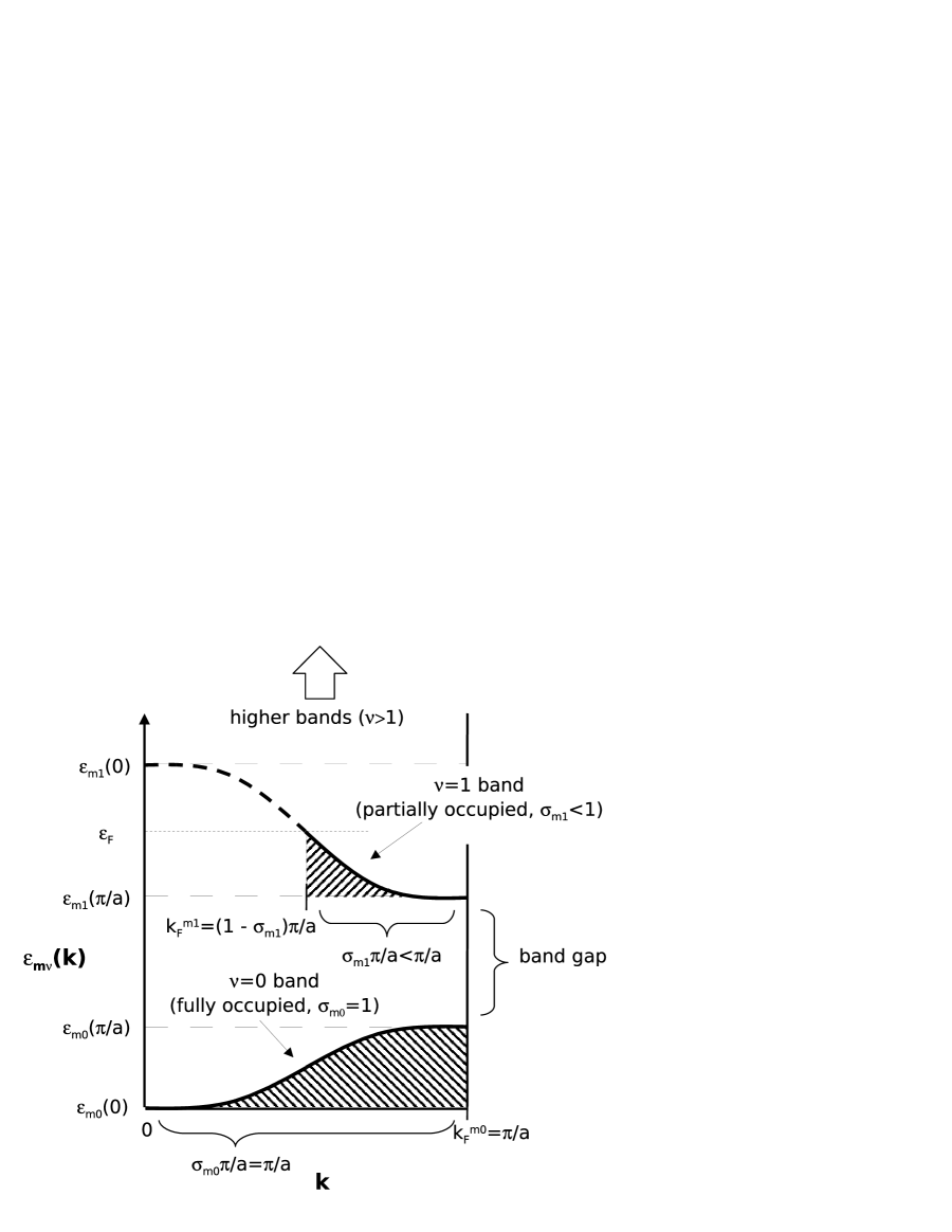
Figure 1: A schematic diagram showing the electron band structure for a particular $m$ value. In this example, the first band ($\nu=0$) is fully occupied ($\sigma_{m0}=1$) while the second band ($\nu=1$) is partially filled ($\sigma_{m1}<1$).

Also shown in the figure is the Fermi level energy $\varepsilon_{F}$ of the electrons in the infinite chain. The electrons occupy all orbitals $(m\nu k)$ with energy less than $\varepsilon_{F}$. For each $(m\nu)$ band, we define the occupation parameter $\sigma_{m\nu}$, which gives the number of electrons that occupy this band per unit cell [i.e., the number of electrons that occupy the $(m\nu)$ band in the whole chain is $\sigma_{m\nu}N$]. Since the maximum possible number of electrons in each $(m\nu)$ band is $N$, we have $\sigma_{m\nu}\leq 1$. Because there are $ZN$ electrons total in the chain, these occupation numbers are subject to the constraint

$$\sum_{m\nu}\sigma_{m\nu}=Z\,.$$ (43)

It is also useful to define for each $(m\nu)$ level the Fermi wave number $k_{F}^{m\nu}$, such that the electrons fill up all allowed orbitals between the minimum-energy Bragg point ($k=0$ for even $\nu$ and $k=\pi/a$ for odd $\nu$) and $k_{F}^{m\nu}$. The occupied $k$’s are therefore

$$k\in\left[0,\sigma_{m\nu}\frac{\pi}{a}\right]\equiv\left[0,k_{F}^{m\nu}\right]$$ (44)

for even $\nu$, and

$$k\in\left[(1-\sigma_{m\nu})\frac{\pi}{a},\frac{\pi}{a}\right]\equiv\left[k_{F}^{m\nu},\frac{\pi}{a}\right]$$ (45)

for odd $\nu$, plus the corresponding reflection about the Bragg point $k=0$. For a completely filled band (as illustrated in Fig. 1 for the $\nu=0$ band), $\sigma_{m\nu}=1$ and $k_{F}^{m\nu}=\pi/a$ (for $\nu=$ even) or $0$ (for $\nu=$ odd); for a partially filled band (the $\nu=1$ band in Fig. 1),

$$\varepsilon_{m\nu}(k_{F}^{m\nu})=\varepsilon_{F}\,.$$ (46)

With the allowed $k$ values specified, the $k$ integration domain in Eqs. (14), (15), (37) and (42) is given by

$$\int_{I_{m\nu}}dk\Rightarrow\left\{\begin{array}[]{ll}2\int_{0}^{k_{F}^{m\nu}}dk,&\mbox{ $\nu$ even,}\\ 2\int_{k_{F}^{m\nu}}^{\pi/a}dk\,,&\mbox{ $\nu$ odd.}\end{array}\right.$$ (47)

Note that the Fermi level energy $\varepsilon_{F}$ and various occupation numbers $\sigma_{m\nu}$ must be calculated self-consistently. In principle, they should be determined by minimizing the total energy with respect to $\sigma_{m\nu}$ subject to the constraint Eq. (43), i.e.,

$$\frac{\delta}{\delta\sigma_{m\nu}}\left[E[n;\sigma_{m\nu}]-\varepsilon_{F}\left(\sum_{m\nu}\sigma_{m\nu}-Z\right)\right]=0\,.$$ (48)

Since

$$\frac{\partial n(\mathbf{r})}{\partial\sigma_{m\nu}}=\pm\frac{\pi}{a}\frac{\partial n(\mathbf{r})}{\partial k_{F}^{m\nu}}=|W_{m}|^{2}(\rho)|f_{m\nu k_{F}^{m\nu}}(z)|^{2},$$ (49)

Eq. (48) yields

$$\left[-\frac{\hbar^{2}}{2m_{e}}\frac{d^{2}}{dz^{2}}+{\bar{V}}_{\rm eff}(z)\right]f_{m\nu k_{F}^{m\nu}}(z)=\varepsilon_{F}f_{m\nu k_{F}^{m\nu}}(z)\,.$$ (50)

Comparing this to Eq. (35), we find $\varepsilon_{m\nu}(k_{F}^{m\nu})=\varepsilon_{F}$, which is Eq. (46). This shows that using Eq. (46) to find $\varepsilon_{F}$ minimizes the total energy of the system.

Figure 2: A schematic diagram showing the shapes of the longitudinal wave functions of electrons in different bands at $k=0$ and $k=\pi/a$.

III.3 The complex longitudinal wave functions

The longitudinal electron wave function $f_{m\nu k}(z)$ satisfies the Kohn-Sham equations (35) subject to the periodicity condition Eq. (13), or equivalently, the cell boundary condition

$$f_{m\nu k}(a/2)=e^{ika}f_{m\nu k}(-a/2)\,.$$ (51)

Since the electron density distribution $n(\mathbf{r})$ is periodic across each cell and symmetric about each ion, the following boundary condition is also useful:

$$|f_{m\nu k}(z)|^{\prime}|_{z=a/2}=|f_{m\nu k}(z)|^{\prime}|_{z=-a/2}=0.$$ (52)

Due to the complex boundary condition Eq. (51), the wave function $f_{m\nu k}$ is complex for general $k$’s. The exceptions are $k=0$ and $k=\pi/a$: For $k=0$, the boundary condition becomes $f_{m\nu k}(a/2)=f_{m\nu k}(-a/2)$, and for $k=\pi/a$ we have $f_{m\nu k}(a/2)=-f_{m\nu k}(-a/2)$. Thus for $k=0$ and $\pi/a$, we can choose the longitudinal wave functions to be real. The general shapes of these wave functions (for different bands) are sketched out in Fig. 2. We see that at the Bragg points, between the two states with the same number of nodes, the one that is more concentrated near the ion has lower energy than the other state; this difference gives rise to the band gap. The $k=0,\pi/a$ eigenvalues $\varepsilon_{m\nu}$ and eigenfunctions can be calculated in the domain $0<z<a/2$ with the boundary condition $f_{m\nu k}(0)=0$ or $f^{\prime}_{m\nu k}(0)=0$.

The electron wave functions for general $k$’s are more difficult to compute as they have complex boundary conditions. Our procedure for calculating these wave functions and their corresponding electron energies is as follows: For each energy band $(m\nu)$, the electron eigenstates at $k=0$ and $k=\pi/a$ are first found (see above). For every energy between $\varepsilon_{m\nu}(k=0)$ and $\varepsilon_{m\nu}(k=\pi/a)$, we find the wave function that solves the Kohn-Sham equation while satisfying the symmetric/periodic density condition Eq. (52). More precisely, we choose $f=1$ (up to a normalization constant) and guess $f^{\prime}=i\,g$ (where $g$ is a real number) at $z=a/2$ (thus $|f|^{\prime}=0$ is satisfied at $z=a/2$), and then integrate the Kohn-Sham equation to $z=-a/2$; we adjust $g$ so that $|f|^{\prime}=0$ is satisfied at $z=-a/2$. Once the wave function is obtained, we determine its $k$ value from the Bloch boundary condition Eq. (51). Through this method we find $\varepsilon_{m\nu}(k)$ as a function of $k$ for each $(m\nu)$ band.

Some examples of our computed $\varepsilon_{m\nu}(k)$ are shown in Figs. 3 and 4. To show that our calculations are consistent with theoretical models, we have included several model fits for the electron energy curves: the tight-binding fit in Fig. 3, which has the form

$$\varepsilon_{m\nu}(k)\simeq c_{1}+c_{2}\cos(ka)$$ (53)

[see Ref. (ashcr76, ), Eq. (10.19)], and the weak-periodic-potential fit in Fig. 4, which has the form

$$\varepsilon_{m\nu}(k)\simeq c_{1}+\frac{1}{2}[k^{2}/2+(2\pi/a-k)^{2}/2]-\frac{1}{2}\{[(2\pi/a-k)^{2}/2-k^{2}/2]^{2}+c_{2}^{2}\}^{1/2}$$ (54)

[see Ref. (ashcr76, ), Eq. (9.26)]. The constants $c_{1}$ and $c_{2}$ in the formulas are fit to the two endpoints of the energy curves, $\varepsilon_{m\nu}(0)$ and $\varepsilon_{m\nu}(\pi/a)$. The tight-binding model fits well for the most-tightly-bound electron bands in our calculations, while the weak-periodic-potential model fits well for all of the other bands. Note that for $k\ll\pi/a$, the electron energy can be approximately fit by $\varepsilon_{m\nu}(k)=\varepsilon_{m\nu}(0)+k^{2}/2$, as would be the case if the wave functions were of the form $f_{m\nu}(z)e^{ikz}$ — this is the ansatz adopted by Neuhauser et al. (1987) in their Hartree-Fock calculations. But obviously for larger $k$, this is a rather bad approximation. We suggest that approximate treatment in the band structure may account for a large part of the discrepancies among cohesive energy results in previous works. For example, the disagreement between Ref. (Jones, 1985) [where $\varepsilon_{m\nu}(k)$ was calculated for a few values of $k$ and then fit to a simple expression] and Ref. (Neuhauser et al., 1987) (where a $k^{2}$ dependence for the electron energy was assumed) on whether or not carbon is bound at $B_{12}=5$ is due to the band structure model, not to the fact the former used the density functional theory while the latter used the Hartree-Fock method.

Figure 3: The electron energy of the $(m,\nu)=(0,0)$ band for the carbon infinite chain at $B_{12}=1$. The tight-binding model fit for this level is shown as a dashed line [see Eq. (53)], and the dotted line shows the free electron result $\varepsilon_{00}(k)-\varepsilon_{00}(0)=k^{2}/2$.

Figure 4: The electron energy of the $(m,\nu)=(0,0)$ band for the iron infinite chain at $B_{12}=2000$. The weak-periodic-potential model fit for this level is shown as a dashed line [see Eq. (54)], and the dotted line shows the free electron result $\varepsilon_{00}(k)-\varepsilon_{00}(0)=k^{2}/2$.

IV Results: One-dimensional chains

In this section we present our results for hydrogen, helium, carbon, and iron infinite chains at various magnetic field strengths between $B=10^{12}$ G and $2\times 10^{15}$ G. For each chain, data is given in tabular form for the ground-state energy (per unit cell) $E_{\infty}$, the equilibrium ion separation $a$, and the electron Fermi level energy $\varepsilon_{F}$ (the electron work function is $W=|\varepsilon_{F}|$). We provide relevant information for the electron occupations in different bands, such as the number of Landau orbitals and the number of fully occupied bands (see below for specific elements). We also give the ground-state energy of the corresponding atom, $E_{a}$, so that the cohesive energy of each chain can be obtained, $Q_{\infty}=E_{a}-E_{\infty}$.

For each chain and atom we provide numerical scaling relations for the ground-state energy and Fermi level energy as a function of the magnetic field, in the form of scaling exponents $\beta$ and $\gamma$, with

$$E_{a},~{}E_{\infty}\propto B^{\beta},\qquad\varepsilon_{F}\propto B^{\gamma}.$$ (55)

We also give the rescaled, dimensionless energy $\bar{E}_{\infty}$, and equilibrium ion separation $\bar{a}$ defined by [see Eq. (3)]

$$E_{\infty}\simeq\bar{E}_{\infty}\,Z^{9/5}b^{2/5}~{}{\rm a.u.},\qquad a\simeq\bar{a}\,Z^{1/5}b^{-2/5}~{}{\rm a.u.}.$$ (56)

We shall see that the scaling relations in Eq. (56) with $\bar{E}_{\infty}\simeq$ const. and $\bar{a}\simeq$ const. represent a reasonable approximation to our numerical results, although such scaling formulae are not accurate enough for calculating the cohesive energy $Q_{\infty}=E_{a}-E_{\infty}$. However, Eq. (4) or Eq. (9) for the Fermi level energy based on the uniform gas model is not a good representation of our numerical results. In paper I (Medin and Lai, 2006) we have shown that as $N$ increases, the energy per atom in the H_N (or He_N, C_N, Fe_N) molecule, $E_{N}/N$, gradually approaches a constant value. The infinite chain ground-state energy $E_{\infty}$ found in the present paper is consistent with the large-$N$ molecule ground-state energy limit $E_{N}/N$ obtained in paper I (see the related figures in the following subsections). Since finite molecules and infinite chains involve completely different treatments of the electron states, the consistency of $E_{\infty}$ and $E_{N}/N$ provides an important check of the validity of our calculations.

Other comparisons can be made between the infinite chains and finite molecules. For example, our results of ion separation $a$ and scaling constant $\beta$ are consistent between infinite chains and finite molecules. Also, we find that if the isolated atom has electrons in $\nu=0$ and $\nu=1$ orbitals, then the corresponding infinite chain will have electrons in $\nu=0$ and $\nu=1$ bands; if the isolated atom only has electrons in $\nu=0$ orbitals, the corresponding infinite chain will have electrons only in $\nu=0$ bands.

We have compared our cohesive energy results with those of other work, whenever available. These comparisons are presented in the following subsections.

IV.1 Hydrogen

Our numerical results for H are given in Table 1. Examples of the energy curves of various H_N molecules and H_∞ at $B_{12}=1$ are depicted in Fig. 5. The minimum of each energy curve determines the equilibrium ion separation in the molecule/chain. Figure 6 compares the molecular and infinite chain energies at various field strengths, and shows that as $N$ increases, the energy per atom in the H_N molecule asymptotes to $E_{\infty}$. Figure 7 gives the occupation number $\sigma_{m0}$ of different Landau orbitals at various field strengths. Only the $\nu=0$ bands are occupied, none of these are completely filled ($\sigma_{m0}<1$), and the $\nu\geq 1$ bands are empty ($\sigma_{m1}=0$). We see that as $B$ increases, the electrons spread into more Landau orbitals, thus the number of $m$ states occupied by the electrons ($n_{m}$ in Table 1) increases. Approximately, since the chain radius $R\propto b^{-2/5}$ and $R\sim(2n_{m}-1)^{1/2}/b^{1/2}$ (the electrons occupy the Landau orbitals with $m=0,1,2,\ldots,n_{m}-1$), we have $n_{m}\propto b^{1/5}$. Table 1 shows that for $B_{12}\gtrsim 10$ our results for $E_{\infty}$ and $a$ are well fit by

$$E_{\infty}\simeq-529\,B_{13}^{0.374}~{}{\rm eV},\qquad a=0.091\,B_{13}^{-0.40}~{}{\rm}a_{0}$$ (57)

[where $B_{13}=B/(10^{13}~{}{\rm G})$], similar to the scaling of Eq. (56). The electron work function $W=|\varepsilon_{F}|$ does not scale as Eq. (4), but is a fraction of the ionization energy of the H atom, $|E_{a}|$. Note that $|E_{a}|$ is not well fit by a power law ($\propto B^{\beta}$), but is well described by $|E_{a}|\propto(\ln b)^{2}$ (accurate fitting formulae for $|E_{a}|$ are given in, e.g., Ref. (ho03, )).

At $B_{12}=1,10,100$, we find cohesive energies of $Q_{\infty}=E_{a}-E_{\infty}=59.6$, $219.7$, $712.7$ eV (see Table 1). At those same fields, Lai et al. (1992) find cohesive energies of $28.9$, $141$, $520$ eV. At $B_{12}=0.94$, Relovsky and Ruder (1996) find a cohesive energy of $47.1$ eV. We expect our H calculation (and that of Ref. (Relovsky and Ruder, 1996)) to overestimate the cohesive energy since an exchange-correlation functional is used in the chain calculation while none is required for the H atom. But we also expect the result obtained in Ref. (Lai et al., 1992) to somewhat underestimate the cohesive energy since a uniform (longitudinal) electron density was assumed.

Table 1: The ground-state energy (per unit cell) $E_{\infty}$ (in units of eV), ion separation $a$ (in units of Bohr radius $a_{0}$), the number of occupied Landau levels $n_{m}$, and the Fermi level energy $\varepsilon_{F}$ (in eV) of 1D infinite chains of hydrogen, over a range of magnetic field strengths. The ground-state energy of individual hydrogen atoms, $E_{a}$ (in units of eV), is also provided for reference. The dimensionless energy $\bar{E}_{\infty}$ and ion separation $\bar{a}$ are calculated using Eq. (56). The scaling exponents $\beta$ and $\gamma$, defined by $E_{a},~{}E_{\infty}\propto B^{\beta}$, and $\varepsilon_{F}\propto B^{\gamma}$, are calculated over the three magnetic field ranges provided in the table: $B_{12}=1-10$, $10-100$, $100-1000$ (the exponent in the $B_{12}=1$ row corresponds to the fit over $B_{12}=1-10$, etc.). The occupation of different $(m\nu)$ bands is designated by the number $n_{m}$: the electrons occupy Landau orbitals with $m=0,1,2,\ldots,n_{m}-1$, all in the $\nu=0$ band; see Fig. 7.

	H			H∞
$B_{12}$	$\quad E_{a}\quad$		$\beta$	$\quad E_{\infty}\quad$		$\bar{E}_{\infty}$	$\beta$	$a$	$\bar{a}$	$n_{m}$	$\varepsilon_{F}$	$\gamma$
1	-161	.4	0.283	-221	.0	-0.721	0.379	0.23	2.6	6	-85.0	0.28
10	-309	.5	0.242	-529	.2	-0.688	0.374	0.091	2.6	10	-165	0.27
100	-540	.3	0.207	-1253	.0	-0.648	0.374	0.037	2.6	16	-311	0.26
1000	-869	.6	-	-2962		-0.610	-	0.0145	2.6	26	-571	-

Figure 5: The energies (per atom or cell) of various H molecules and infinite chain as a function of ion separation $a$ at $B_{12}=1$. The results of finite molecules are based on paper I (Medin and Lai, 2006). The energy of the H atom is shown as a horizontal line at $-161.4$ eV.

Figure 6: The molecular energy per atom, $|E_{N}|/N$, for the H_N molecule, as a function of $N$ at several different field strengths. The results of finite molecules are based on paper I (Medin and Lai, 2006). As $N$ increases, $E_{N}/N$ asymptotes to $E_{\infty}$. To facilitate plotting, the values of $|E_{1}|$ (atom) at different magnetic field strengths are normalized to the value at $B_{12}=1$, $161.4$ eV. This means that $\alpha=1$ for $B_{12}=1$, $\alpha=161.4/309.5$ for $B_{12}=10$, $\alpha=161.4/540.3$ for $B_{12}=100$, and $\alpha=161.4/869.6$ for $B_{12}=1000$.

Figure 7: The occupation numbers of each $m$ level of hydrogen infinite chains, for various magnetic field strengths. The data points are plotted over the curves to show the discrete nature of the $m$ levels. Note that only the $\nu=0$ bands are occupied by the electrons.

IV.2 Helium

Our numerical results for He are given in Table 2. Figure 8 compares the molecular and infinite chain energies at various field strengths, and shows that as $N$ increase, the energy per atom in the He_N molecule approaches $E_{\infty}$ for the infinite chain. Figure 9 gives occupation number $\sigma_{m0}$ of different Landau orbitals at various field strengths. As in the case of H, only the $\nu=0$ bands are occupied, and the number of Landau states required ($n_{m}$ in Table 2) increases with increasing $B$, with $n_{m}\propto Z^{2/5}b^{1/5}$. Table 2 shows that for $B_{12}\gtrsim 10$,

$$E_{\infty}\simeq-1252\,B_{13}^{0.382}~{}{\rm eV},\qquad a=0.109\,B_{13}^{-0.40}~{}{\rm}a_{0}\,,$$ (58)

similar to the scaling of Eq. (56). The electron work function $W=|\varepsilon_{F}|$ does not scale as Eq. (4), but is a fraction of the ionization energy: Using a Hartree-Fock code (e.g., Ref. (Lai et al., 1992)) we find that at $B_{12}=1,10,100,1000$ the He atomic energies are $-575.5$, $-1178.0$, $-2193$, $-3742$ eV. The He⁺ (i.e., once-ionized He) energies at these field strengths are $-416.2$, $-846.5$, $-1562.0$, $-2638$ eV. Therefore, the ionization energies of He at these field strengths are $159.3$, $331.5$, $631$, and $1104$ eV, respectively.

At $B_{12}=1$, we find a cohesive energy of $58.9$ eV (see Table 2). At the same field, Neuhauser et al. (1987) (based on the Hartree-Fock model) find a cohesive energy of $25$ eV, and Müller (1984) (based on variational methods) gives a cohesive energy of $50$ eV. At $B_{12}=0.94$, Relovsky and Ruder (1996) (based on density functional theory) find a cohesive energy of $56.6$ eV. At $B_{12}=5$ Jones (1985) finds a cohesive energy of $220$ eV, which is close to our value. That our results agree best with those of Refs. (Relovsky and Ruder, 1996; Jones, 1985) is expected, as we used a similar method to find the ground-state atomic and chain energies. Similar to the finite He molecules (paper I), we expect our density-functional-theory calculation to overestimate the cohesive energy, but we also expect the result of Ref. (Neuhauser et al., 1987) to underestimate $Q_{\infty}$.

Table 2: The ground-state energy (per unit cell) $E_{\infty}$ (in units of eV), ion separation $a$ (in units of Bohr radius $a_{0}$), the number of occupied Landau levels $n_{m}$, and Fermi level energy $\varepsilon_{F}$ (in eV) of 1D infinite chains of helium, over a range of magnetic field strengths. The ground-state energy of individual He atoms, $E_{a}$ (in units of eV), is also provided for reference (this is based on the density-functional-theory calculation of Ref. (Medin and Lai, 2006)). The dimensionless energy $\bar{E}_{\infty}$ and ion separation $\bar{a}$ are calculated using Eq. (56). The scaling exponents $\beta$ and $\gamma$, defined by $E_{a},~{}E_{\infty}\propto B^{\beta}$, and $\varepsilon_{F}\propto B^{\gamma}$, are calculated over the three magnetic field ranges provided in the table: $B_{12}=1-10$, $10-100$, $100-1000$ (the exponent in the $B_{12}=1$ row corresponds to the fit over $B_{12}=1-10$, etc.). The occupation of different $(m\nu)$ bands is designated by the number $n_{m}$: the electrons occupy Landau orbitals with $m=0,1,2,\ldots,n_{m}-1$, all in the $\nu=0$ band; see Fig. 9. Note that all of the He atoms here also have electrons only in the $\nu=0$ states.

	He			He∞
$B_{12}$	$E_{a}$		$\beta$	$E_{\infty}$		$\bar{E}_{\infty}$	$\beta$	$a$	$\bar{a}$	$n_{m}$	$\varepsilon_{F}$	$\gamma$
1	-603	.5	0.317	-662	.4	-0.621	0.385	0.28	2.7	9	-85.0	0.29
10	-1252	.0	0.280	-1608	.0	-0.600	0.382	0.109	2.7	14	-167	0.27
100	-2385		0.248	-3874		-0.575	0.382	0.043	2.7	23	-310	0.26
1000	-4222		-	-9329		-0.552	-	0.0175	2.7	39	-568	-

Figure 8: The molecular energy per atom, $|E_{N}|/N$, for the He_N molecule, as a function of $N$ at several different field strengths. The results of finite molecules are based on paper I (Medin and Lai, 2006). As $N$ increases, $E_{N}/N$ asymptotes to $E_{\infty}$. To facilitate plotting, the values of $|E_{1}|$ (atom) at different magnetic field strengths are normalized to the value at $B_{12}=1$, $603.5$ eV. This means that $\alpha=1$ for $B_{12}=1$, $\alpha=603.5/1252.0$ for $B_{12}=10$, $\alpha=603.5/2385$ for $B_{12}=100$, and $\alpha=603.5/4222$ for $B_{12}=1000$.

Figure 9: The occupation numbers of each $m$ level of infinite He chains, for various magnetic field strengths. Only the $\nu=0$ bands are occupied by the electrons. Note that for $B_{12}=1$, the $m=8$ orbital has a rather small occupation, $\sigma_{80}\simeq 0.006$; if $\varepsilon_{F}$ were slightly more negative, this orbital would be completely unoccupied.

IV.3 Carbon

Our numerical results for C are given in Table 3. Figure 10 compares molecular and infinite chain energies at various field strengths, showing that as $N$ increase, the energy per atom in the C_N molecule approaches $E_{\infty}$ for the infinite chain. Figure 11 gives the occupation number $\sigma_{m0}$ of different Landau orbitals at various field strengths. As in the case of H and He, only the $\nu=0$ bands are occupied, although for C at $B_{12}=1$, the $m=0$ and $m=1$ bands (both with $\nu=0$) are fully occupied (thus $n_{f}=2$ in Table 3). The number of Landau states required ($n_{m}$ in Table 3) increases with increasing $B$, approximately with $n_{m}\propto Z^{2/5}b^{1/5}$. Table 3 shows that for $B_{12}\gtrsim 10$,

$$E_{\infty}\simeq-10\,300\,B_{13}^{0.387}~{}{\rm eV},\qquad a=0.154\,B_{13}^{-0.43}~{}{\rm}a_{0}\,.$$ (59)

Note that these expressions are more approximate than for H and He. The electron work function $W=|\varepsilon_{F}|$ does not scale as Eq. (4), but is a fraction of the ionization energy: from paper I (Medin and Lai, 2006), the ionization energies of C at $B_{12}=1,10,100,1000$ are $174$, $430$, $990$, and $2120$ eV, respectively.

At $B_{12}=10$, we find a cohesive energy of $240$ eV (see Table 3). At $B_{12}=8.5$, Relovsky and Ruder (1996) give a cohesive energy of $240$ eV. At $B_{12}=5$ Jones (1985) finds a cohesive energy of $100$ eV; at the same field (using our scaling relations), we find a cohesive energy of $100$ eV ($\pm 30$ eV). Neuhauser et al. (1987), on the other hand, find that carbon is not bound at $B_{12}=1$ or $5$. This is probably due to the approximate band structure ansatz adopted in Ref. (Neuhauser et al., 1987) (see Sec. III.3): for fully occupied bands, the approximation that $\varepsilon_{m\nu}(k)$ increases as $k^{2}/2$ is invalid and can lead to large error in the total energy of the chain.

Table 3: The ground-state energy (per unit cell) $E_{\infty}$ (in units of eV), ion separation $a$ (in units of Bohr radius $a_{0}$), electron occupation numbers ($n_{m},n_{f}$), and Fermi level energy $\varepsilon_{F}$ (in eV) of 1D infinite chains of carbon, over a range of magnetic field strengths. The ground-state energy of individual C atoms, $E_{a}$ (in units of eV), is also provided for reference (this is based on the density-functional-theory calculation of Ref. (Medin and Lai, 2006)). The dimensionless energy $\bar{E}_{\infty}$ and ion separation $\bar{a}$ are calculated using Eq. (56). The scaling exponents $\beta$ and $\gamma$, defined by $E_{a},~{}E_{\infty}\propto B^{\beta}$, and $\varepsilon_{F}\propto B^{\gamma}$, are calculated over the three magnetic field ranges provided in the table: $B_{12}=1-10$, $10-100$, $100-1000$ (the exponent in the $B_{12}=1$ row corresponds to the fit over $B_{12}=1-10$, etc.). The occupation of different $(m\nu)$ bands is designated by the notation $(n_{m},n_{f})$: the electrons occupy Landau orbitals with $m=0,1,2,\ldots,n_{m}-1$, all with $\nu=0$; the number of fully occupied ($\sigma_{m\nu}=1$) bands is denoted by $n_{f}$; see Fig. 11. Note that all of the C atoms here also have electrons only in the $\nu=0$ states.

	C		C∞
$B_{12}$	$E_{a}$	$\beta$	$E_{\infty}$	$\bar{E}_{\infty}$	$\beta$	$a$	$\bar{a}$	$(n_{m},n_{f})$	$\varepsilon_{F}$	$\gamma$
1	-4341	0.366	-4367	-0.567	0.373	0.49	3.9	(12,2)	-92.8	0.27
10	-10075	0.326	-10315	-0.533	0.385	0.154	3.1	(23,0)	-173	0.25
100	-21360	0.287	-25040	-0.515	0.389	0.056	2.8	(41,0)	-306	0.25
1000	-41330	-	-61320	-0.502	-	0.022	2.7	(69,0)	-539	-

Figure 10: The molecular energy per atom, $|E_{N}|/N$, for the C_N molecule, as a function of $N$ at several different field strengths. The results of finite molecules are based on paper I (Medin and Lai, 2006). As $N$ increases, $E_{N}/N$ asymptotes to $E_{\infty}$. To facilitate plotting, the values of $|E_{1}|$ (atom) at different magnetic field strengths are normalized to the value at $B_{12}=1$, $4341$ eV. This means that $\alpha=1$ for $B_{12}=1$, $\alpha=4341/10\,075$ for $B_{12}=10$, $\alpha=4341/21\,360$ for $B_{12}=100$, and $\alpha=4341/41\,330$ for $B_{12}=1000$.

Figure 11: The occupation numbers of each $m$ level of infinite C chains, for various magnetic field strengths. Only the $\nu=0$ bands are occupied by the electrons. Note that for $B_{12}=1$, the $m=0$ and $m=1$ bands are completely filled.

IV.4 Iron

Our numerical results for Fe are given in Table 4. The electron density profile at various field strengths is shown in Figs. 12 and 13. As the magnetic field increases the density goes up, for two reasons. First, the equilibrium ion separation decreases. Second, the electrons become more tightly bound to each ion, in both the $\rho$ and $z$ directions (the electrons move closer to each ion faster than the ions move closer to each other). It is interesting to note that the peak density at a given $z$ is not necessarily along the centeral axis of the chain ($\rho=0$), but gradually moves outward with increasing $z$.

The energy curves for Fe₂, Fe₃ (calculated in paper I (Medin and Lai, 2006)), and Fe_∞ at $B_{12}=500$ are shown in Fig. 14. Figure 15 compares the molecular and infinite chain energies at various field strengths, showing that as $N$ increases, the energy per atom in the Fe_N molecule approaches $E_{\infty}$ for the infinite chain. Figure 16 gives the occupation number $\sigma_{m\nu}$ of different bands at various field strengths. For $B_{12}\gtrsim 100$, only the $\nu=0$ bands are occupied; for such field strengths, the Fe atom also has all its electrons in the tightly bound $\nu=0$ states (see Table 4). At $B_{12}=100$, the number of fully occupied bands is $n_{f}^{(0)}=7$ ($m=0,1,2,\ldots,6$, all with $\nu=0$). As $B$ increases, the electrons spread to more Landau orbitals, and the number of occupied $m$-states $n_{m}^{(0)}$ increases, approximately as $n_{m}^{(0)}\propto Z^{2/5}b^{1/5}$. Note that at the highest field strength considered, the electrons occupy $m=0,1,2,\ldots,156$ — keeping track of all these Landau orbitals ($n_{m}^{(0)}=157$) is one of the more challenging aspects of our computation. Table 4 shows that for $B_{12}\gtrsim 100$,

$$E_{\infty}\simeq-356\,B_{14}^{0.374}~{}{\rm keV},\qquad a=0.107\,B_{14}^{-0.43}~{}{\rm}a_{0}$$ (60)

[where $B_{14}=B/(10^{14}~{}{\rm G})$]. These scaling expressions are more approximate than for H and He. The electron work function $W=|\varepsilon_{F}|$ does not scale as Eq. (4), but is a fraction of the ionization energy: from paper I (Medin and Lai, 2006), the ionization energies of Fe at $B_{12}=100,500,1000,2000$ are $1.2$, $2.5$, $3.4$, and $5.5$ keV, respectively.

Note that at $B_{12}=5$ and $10$, the cohesive energy ($Q_{\infty}=E_{a}-E_{\infty}$) of the iron chain is rather small compared to the absolute value of the ground-state energy of the atom ($|E_{a}|$) or chain ($|E_{\infty}|$). For these field strengths, our formal numerical result for the cohesive energy is at or smaller than the standard error of our computations ($0.1\%$ of $|E_{a}|$ or $|E_{\infty}|$), so we have redone the calculations using more grid and integration points such that the atomic and chain energies reported here for these field strengths are accurate to at least $0.02\%$ of $|E_{a}|$ or $|E_{\infty}|$ (see the Appendix). Although these more-accurate cohesive energies are (barely) larger than the error in our calculations, there are of course systematic errors introduced by using density functional theory which must be considered. It is very possible that a similar, full-band-structure calculation using Hartree-Fock theory would find no binding. In any case, for such “low” field strengths ($B_{12}\lesssim 10$) the exact result of our one-dimensional calculation is not crucial, since in the three-dimensional condensed matter the additional cohesion resulting from chain-chain interactions dominates over $Q_{\infty}$, as we will show in Sec. V.

At $B_{12}=5$, Neuhauser et al. (1987) and Jones (1985) found that iron is not bound, while we find that it is barely bound. At $B_{12}=10$, Jones (1986) calculated the cohesive energy for three-dimensional condensed matter, so we compare our results with those of Ref. (Jones, 1986) in Sec. V. We have not found any quantitative calculations of cohesive energies for iron at field strengths larger than $10^{13}$ G.

Table 4: The ground-state energy (per unit cell) $E_{\infty}$ (in units of keV), ion separation $a$ (in units of the Bohr radius $a_{0}$), electron occupation numbers ($n_{m}^{(0)},n_{f}^{(0)};n_{m}^{(1)},n_{f}^{(1)}$), and Fermi level energy $\varepsilon_{F}$ (in eV) of 1D infinite iron chains, over a range of magnetic field strengths. The ground-state energy of individual Fe atoms, $E_{a}$ (in units of keV), is also provided for reference (this is based on the density-functional-theory calculation of Ref. (Medin and Lai, 2006)). The dimensionless energy $\bar{E}_{\infty}$ and ion separation $\bar{a}$ are calculated using Eq. (56). The scaling exponents $\beta$ and $\gamma$, defined by $E_{a},~{}E_{\infty}\propto B^{\beta}$, and $\varepsilon_{F}\propto B^{\gamma}$, are calculated over the three magnetic field ranges provided in the table: $B_{12}=1-10$, $10-100$, $100-1000$ (the exponent in the $B_{12}=1$ row corresponds to the fit over $B_{12}=1-10$, etc.). For atoms the electron configuration is specified by the notation $(n_{0},n_{1})$ (with $n_{0}+n_{1}=Z=26$), where $n_{0}$ is the number of electrons in the $\nu=0$ orbitals and $n_{1}$ is the number of electrons in the $\nu=1$ orbitals. For infinite chains, the occupation of different $(m\nu)$ bands is designated by the notation $(n_{m}^{(0)},n_{f}^{(0)};n_{m}^{(1)},n_{f}^{(1)})$, where $n_{m}^{(0)}$ is the total number of occupied $\nu=0$ orbitals (from $m=0$ to $m=n_{m}^{(0)}-1$), and $n_{m}^{(1)}$ the corresponding number for the $\nu=1$ orbitals; $n_{f}^{(0)}$ ($n_{f}^{(1)}$) is the number of fully occupied ($\sigma_{m\nu}=1$) $\nu=0$ ($\nu=1$) orbitals. Note that for $B_{12}\gtrsim 100$, only the $\nu=0$ states are occupied in the Fe atom, and only the $\nu=0$ bands are occupied in the Fe chain; see Fig. 16.

	Fe				Fe∞
$B_{12}$	$E_{a}$ (keV)		$(n_{0},n_{1})$	$\beta$	$E_{\infty}$ (keV)		$\bar{E}_{\infty}$	$\beta$	$a$	$\bar{a}$	$(n_{m}^{(0)},n_{f}^{(0)};n_{m}^{(1)},n_{f}^{(1)})$	$\varepsilon_{F}$ (eV)	$\gamma$
5	-107	.23	(24,2)	0.407	-107	.31	0.522	0.407	0.42	4.7	(35,15;3,1)	-161	0.27
10	-142	.15	(25,1)	0.396	-142	.30	0.525	0.398	0.30	4.4	(42,13;2,0)	-194	0.30
100	-354	.0	(26,0)	0.366	-355	.8	0.522	0.376	0.107	4.0	(69,7)	-384	0.26
500	-637	.8	(26,0)	0.346	-651	.9	0.503	0.371	0.050	3.5	(105,2)	-583	0.12
1000	-810	.6	(26,0)	0.334	-842	.8	0.493	0.372	0.035	3.3	(130,1)	-635	0.12
2000	-1021	.5	(26,0)	-	-1091	.0	0.483	-	0.025	3.1	(157,0)	-690	-

Figure 12: The density distribution of electrons in the iron infinite chain at four different magnetic field strengths (labeled on the graphs). The density is shown as a function of $\rho$ for five equally spaced $z$ points from the center of a cell ($z=0$) to the edge of that cell ($z=a/2$).

Figure 13: The density distribution of electrons in the iron infinite chain at four different magnetic field strengths (labeled on the graphs). The density is shown as a function of $z$ for five equally spaced $\rho$ points from the center of a cell ($\rho=0$) to the guiding center radius of the highest occupied $m$ level ($\rho=\rho_{m_{\rm max}}$). The $\rho$ points are given in units of $a_{0}$.

Figure 14: The energy per cell as a function of the ion separation for an infinite Fe chain at $B_{12}=500$. The molecular energy per atom versus ion separation for the Fe₂ and Fe₃ molecules at the same field strength (based on calculations in paper I) are also shown. The energy of the Fe atom is shown as a horizontal line at $-637.8$ keV.

Figure 15: The molecular energy per atom, $|E_{N}|/N$, for the Fe_N molecule, as a function of $N$ at several different field strengths. The results of finite molecules are based on paper I (Medin and Lai, 2006). As $N$ increases, $E_{N}/N$ asymptotes to $E_{\infty}$. To facilitate plotting, the values of $|E_{1}|$ (atom) at different magnetic field strengths are normalized to the value at $B_{12}=100$, $354.0$ keV. This means that $\alpha=1$ for $B_{12}=100$, $\alpha=354.0/637.8$ for $B_{12}=500$, $\alpha=354.0/810.6$ for $B_{12}=1000$, and $\alpha=354.0/1021.5$ for $B_{12}=2000$.

Figure 16: The occupation numbers of each $m$ level of infinite Fe chains, for various magnetic field strengths. For $B_{12}\gtrsim 100$, only the $\nu=0$ bands are occupied by the electrons (upper panel). For $B_{12}=5$ and $10$ the $m$ levels with $\nu=1$ are shown with points as well as lines, since there are only a few such occupied levels (lower panel).

V Calculations of three-dimensional condensed matter

For the magnetic field strengths considered in this paper ($B\gtrsim 10^{12}$ G), H and He infinite chains are significantly bound relative to individual atoms. Additional binding energy between 3D condensed matter and 1D chain is expected to be small (Lai et al., 1992) (see below). Thus the cohesive energy of the 3D condensed H or He, $Q_{s}=E_{a}-E_{s}$ (where $E_{s}$ is the energy per cell in the 3D condensed matter), is close to $Q_{\infty}=E_{a}-E_{\infty}$, the cohesive energy of the 1D H or H chain. For C and Fe at relatively low magnetic fields (e.g., C at $B_{12}\lesssim 10$ and Fe at $B_{12}\lesssim 100$), 1D chains are not significantly bound relative to atoms and additional cohesion due to chain-chain interactions is important in determining the true cohesive energy of the 3D condensed matter. Indeed, for Fe at $B_{12}=5,10$, our calculations of 1D chains give such a small $Q_{\infty}$ (see Table 4) that it is somewhat ambiguous as to whether the Fe condensed matter is truly bound relative to individual atoms. In these cases, calculations of 3D condensed matter is crucial (Jones, 1986).

In this section, we present an approximate calculation of the relative binding energy between 3D condensed matter and 1D chains, $\Delta E_{s}=E_{s}-E_{\infty}$.

V.1 Method

To form 3D condensed matter we place the infinite chains in parallel bundles along the magnetic field. We consider a body-centered tetragonal lattice structure; i.e., the chains are uniformly spaced in over a grid in the $xy$ plane (perpendicular to the magnetic axis), with every other chain in the grid shifted by half a cell ($\Delta z=a/2$) in the $z$ direction. The transverse separation between two nearest neighboring chains is denoted by $2R$, with $R$ to be determined.

To calculate the ground-state energy of this 3D condensed matter, we assume that the electron density calculated for an individual 1D chain is not modified by chain-chain interactions, thus we do not solve for the full electron density in the 3D lattice self-consistently. In reality, for each Landau orbital the transverse wave function of an electron in the 3D lattice is no longer given by Eq. (11) (which is centered at one particular chain), but is given by a superposition of many such Landau wave functions centered at different lattice sites and satisfies the periodic (Bloch) boundary condition. The longitudinal wave function $f_{m\nu k}(z)$ will be similarly modified. Our calculations show that the equilibrium separation ($2R$) between chains is large enough that there is little overlap in the electron densities of any two chains, so we believe that our approximation is reasonable.

Using this approximation, the electron density in the 3D lattice is simply the sum of individual infinite chain electron densities:

$$n_{\rm 3D}(\mathbf{r})=\sum_{ij}n(\mathbf{r}-\mathbf{r}_{ij})\,,$$ (61)

where $n(\mathbf{r})$ are the electron density in the 1D chain (as calculated in Secs. III-IV), the sum over $ij$ spans all positive and negative integers, and

$$\mathbf{r}_{ij}=2Ri\,\hat{\mathbf{x}}+2Rj\,\hat{\mathbf{y}}+\frac{a}{2}[i,j]\,\hat{\mathbf{z}}$$ (62)

represents the location of the origin of each chain (the notation $[i,j]=1$ when $i+j=$ odd, and $[i,j]=0$ when $i+j=$ even). In practice, the chain-chain overlap is so small that we only need to consider neighboring chains. The density at a point in the positive $xyz$ octant of a 3D unit cell is approximately given by

$$n_{\rm 3D}(\mathbf{r})\simeq n(\mathbf{r})+n(\mathbf{r}-2R\hat{\mathbf{x}}-a/2\hat{\mathbf{z}})+n(\mathbf{r}-2R\hat{\mathbf{y}}-a/2\hat{\mathbf{z}})+n(\mathbf{r}-2R\hat{\mathbf{x}}-2R\hat{\mathbf{y}})\,.$$ (63)

The energy (per unit cell) $\Delta E_{3D}(R)$ of the 3D condensed matter relative to the 1D chain consists of the chain-chain interaction Coulomb energy $\Delta E_{\rm Coul}$ and the additional electron kinetic energy $\Delta E_{K}$ and exchange-correlation energy $\Delta E_{\rm exc}$ due to the (slight) overlap of different chains. The dominant contribution to the Coulomb energy comes from the interaction between nearest-neighboring cells. For a given cell in the matter, each of the eight nearest-neighboring cells contributes an interaction energy of

$$E_{\rm nn}=E_{eZ,\rm nn}+E_{\rm dir,nn}+E_{ZZ,\rm nn}\,,$$ (64)

where

$$E_{eZ,\rm nn}=-Ze^{2}\int_{|z|<a/2}d\mathbf{r}\,\frac{n(\mathbf{r})}{|\mathbf{r}-\mathbf{r}_{\rm nn}|}\,,$$ (65)

$$E_{\rm dir,nn}[n]=\frac{e^{2}}{2}\int\!\!\int_{|z|<a/2,\,|z^{\prime}|<a/2}d\mathbf{r}\,d\mathbf{r}^{\prime}\,\frac{n(\mathbf{r})n(\mathbf{r}^{\prime})}{|\mathbf{r}-(\mathbf{r}^{\prime}+\mathbf{r}_{\rm nn})|}$$ (66)

$$E_{ZZ,\rm nn}=\frac{1}{2}\frac{Z^{2}e^{2}}{|\mathbf{r}_{\rm nn}|}=\frac{1}{2}\frac{Z^{2}e^{2}}{\sqrt{(a/2)^{2}+(2R)^{2}}}\,,$$ (67)

and $\mathbf{r}_{\rm nn}$ is the location of the ion in a nearest-neighboring cell, for example

$$\mathbf{r}_{\rm nn}=2R\hat{\mathbf{x}}+\frac{a}{2}\,\hat{\mathbf{z}}.$$ (68)

More distant cells contribute to the Coulomb energy through their quadrupole moments. The classical quadrupole-quadrupole interaction energy between two cells separated by a distance $d$ is

$$E_{QQ}(d,\theta)=\frac{3e^{2}}{16}\frac{Q_{zz}^{2}}{d^{5}}(3-30\cos^{2}\theta+35\cos^{4}\theta)\,,$$ (69)

where $Q_{zz}$ is given by Eq. (39) and $\theta$ is the angle between the line joining the two quadrupoles and the $z$ axis. The total contribution from all nonneighboring cells to the Coulomb energy is then

$${1\over 2}\sum_{(ijk)}E_{QQ}({\bf r}_{ijk}),$$ (70)

where

$$\mathbf{r}_{ijk}=\mathbf{r}_{ij}+a\,k\,\hat{\mathbf{z}},\quad d=|{\bf r}_{ijk}|,\quad\cos\theta={k+[i,j]/2\over d/a},$$ (71)

and the sum in Eq. (70) spans over all positive and negative integers except those corresponding to the nearest neighbors.

In the density functional theory, the kinetic and exchange-correlation energies depend entirely on the electron density. These energies differ in the 3D condensed matter from the 1D chain because the overall electron density $n_{\rm 3D}({\bf r})$ [see Eq. (61)] within each 3D cell is (slightly) larger than $n({\bf r})$ due to the overlap of the infinite chains. Since we do not solve for the electron density in the 3D condensed matter self-consistently, we calculate the kinetic energy difference using the local (Thomas-Fermi) approximation:

$$\Delta E_{K}(R)=\int_{|z|<a/2;\,|x|,|y|<R}\!d\mathbf{r}\,n_{\rm 3D}(\mathbf{r})\,\varepsilon_{K}(n_{\rm 3D})-\int_{|z|<a/2}\!d\mathbf{r}\,n(\mathbf{r})\,\varepsilon_{K}(n)\,.$$ (72)

Here $\varepsilon_{K}(n)$ is the (Thomas-Fermi) kinetic energy (per electron) for an electron gas at density $n$, and is given by (e.g., (Lai, 2001))

$$\varepsilon_{K}(n)={\hbar^{2}(2\pi^{2}\rho_{0}^{2}n)^{2}\over 6m_{e}}=\frac{e^{2}}{3\rho_{0}}\,b^{1/2}\,t\,,$$ (73)

where $t$ is given by Eq. (29). Note that the regions of integration in the $xy$ direction are different for the two terms in Eq. (72), as in the 1D chain the unit cell extends over all $\rho$ space, while in the 3D condensed matter the cell is restricted to $x,y\in[-R,R]$.

Similar to $\Delta E_{K}$, in the local approximation, the change in exchange-correlation energy per unit cell is

$$\Delta E_{\rm exc}(R)=\int_{|z|<a/2;\,|x|,|y|<R}\!d\mathbf{r}\,n_{\rm 3D}(\mathbf{r})\,\varepsilon_{\rm exc}(n_{\rm 3D})-\int_{|z|<a/2}\!d\mathbf{r}\,n(\mathbf{r})\,\varepsilon_{\rm exc}(n)\,,$$ (74)

where $\varepsilon_{\rm exc}(n)$ is the exchange-correlation energy (per electron) at density $n$ (see Sec. III.1).

Combining the Coulomb energy, the kinetic energy, and the exchange-correlation energy, the total change in the energy per unit cell when 3D condensed matter is formed from 1D infinite chains can be written

$$\Delta E_{\rm 3D}(R)=\Delta E_{\rm Coul}+\Delta E_{K}+\Delta E_{\rm exc}\,,$$ (75)

where

$$\Delta E_{\rm Coul}(R)=8E_{\rm nn}+{1\over 2}\sum_{(ijk)}E_{QQ}({\bf r}_{ijk})\,.$$ (76)

We calculate $\Delta E_{\rm 3D}(R)$ as a function of $R$ and locate the minimum to determine the equilibrium chain-chain separation $2R$ and the equilibrium energy of the 3D condensed matter. Our method for evaluating various integrals is described in the appendix.

V.2 Results: 3D condensed matter

Table 5 presents our numerical results for the equilibrium chain-chain separation $2R=2R_{\rm eq}$ and the energy difference (per cell) between the 3D condensed matter and 1D chain, $\Delta E_{s}=E_{s}-E_{\infty}=\Delta E_{\rm 3D}(R=R_{\rm eq})$, for C and Fe at various magnetic field strengths. A typical energy curve is shown in Fig. 17. We see that it is important to include the kinetic energy contribution $\Delta E_{K}$ to the 3D energy; without $\Delta E_{K}$, the energy curve would not have a local minimum at a finite $R$.

A comparison of the $R$ values in Table 5 with various iron chain electron densities in Fig. 12 shows that our assumption of small electron density overlap between chains is indeed a good approximation. The electron densities are slowly-varying at the overlapping region, so using the local (Thomas-Fermi) model to calculate the kinetic energy difference is also consistent with the results of our model. Our equilibrium $R$ is within about $15\%$ of the value predicted in the uniform cylinder model [see Eq. (3)].

Table 5: The energy difference (per unit cell) between the 3D condensed matter and 1D chain, $\Delta E_{s}=E_{s}-E_{\infty}$, for carbon and iron over a range of magnetic field strengths. Energies are given in units of eV for C and keV for Fe. The equilibrium chain-chain separation is $2R$ (in units of the Bohr radius $a_{0}$).

	C		Fe
$B_{12}$	$\Delta E_{s}$	$R$	$\Delta E_{s}$		$R$
	(eV)		(   keV)
1	-30	0.200
5	-40	0.110	-0	.6	0.150
10	-20	0.094	-0	.6	0.115
100	-20	0.041	-2	.2	0.054
500	-30	0.022	-2	.1	0.025
1000	-10	0.017	-1	.3	0.021

Figure 17: The energy (per cell) of 3D condensed matter relative to 1D chain as a function of $R$, for carbon at $B_{12}=1$. The nearest-neighbor chain-chain separation in the 3D condensed matter is $2R$. The solid curve gives $\Delta E_{\rm 3D}(R)$ [Eq. (75)] and the dashed curve gives only the Coulomb energy $\Delta E_{\rm Coul}$ [Eq. (76)].

Given our results for $\Delta E_{s}$ and the cohesive energy of 1D chains, $Q_{\infty}=E_{a}-E_{\infty}$, we can obtain the cohesive energy of 3D condensed matter from

$$Q_{s}=E_{a}-E_{s}=E_{a}-(E_{\infty}+\Delta E_{s})=Q_{\infty}-\Delta E_{s}\,.$$ (77)

For H and He, we find that $|\Delta E_{s}|$ is small compared to $Q_{\infty}$ and thus $Q_{s}\simeq Q_{\infty}$. Figure 18 depicts $Q_{s}$ and $Q_{\infty}$ as a function of $B$ for H, He, C, and Fe.

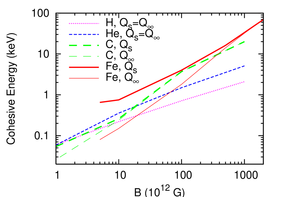
Figure 18: The cohesive energy as a function of $B$, for H (dotted line) and He (short-dashed line) infinite chains and C (long-dashed lines) and Fe (solid lines) infinite chains (lighter lines) and 3D condensed matter (heavier lines).

The only previous quantitative calculation of 3D condensed matter is that by Jones (1986), who finds cohesive energies of $Q_{s}=0.60$, $0.92$ keV for iron at $B_{12}=5,10$. At these field strengths, our calculation (see Tables 4 and 5) gives $Q_{s}=E_{a}-E_{s}=Q_{\infty}-\Delta E_{s}=0.08+0.6\simeq 0.7$ keV and $0.15+0.6\simeq 0.75$ keV, respectively.

Note that our calculations and the results presented here assume that the ion spacing along the magnetic axis in 3D condensed matter, $a$, is the same as in the 1D chain. We have found that if both $a$ and $R$ are allowed to vary, the 3D condensed matter energy can be lowered slightly. This correction is most important for relatively low field strengths. For example, in the case of Fe at $B_{12}=10$, if we increase $a$ from the 1D chain value by $10\%$, then $Q_{\infty}$ decreases by about $50$ eV, but $|\Delta E_{s}|$ increases by about $200$ eV, so that $Q_{s}$ is increased to $\sim 0.9$ keV. Given the approximate nature of our 3D calculations, we do not explore such refinement in detail in this paper.

VI Discussions

Using density functional theory, we have carried out extensive calculations of the cohesive properties of 1D infinite chains and 3D zero-pressure condensed matter in strong magnetic fields. Our results, presented in various tables, figures, and fitting formulae, show that hydrogen, helium, and carbon infinite chains are all bound relative to individual atoms for magnetic fields $B\geq 10^{12}$ G, but iron chains are not (significantly) bound until around $B\sim 10^{14}$ G. For a given zero-pressure condensed matter system, the cohesion along the magnetic axis (chain axis) dominates over chain-chain interactions across the magnetic axis at sufficiently strong magnetic fields. But for relative low field strengths (e.g. Fe at $B\lesssim 10^{14}$ G and C at $B\lesssim{\rm a~{}few}\times 10^{12}$ G), chain-chain interactions play an important role in the cohesion of 3D condensed matter. Our calculations show that for the field strengths considered in this paper ($B\gtrsim 10^{12}$ G), 3D condensed H, He, C and Fe are all bound relative to individual atoms: For C, the cohesive energy $Q_{s}=E_{a}-E_{c}$ ranges from $\sim 50$ eV at $B=10^{12}$ G to $20$ keV at $10^{15}$ G; for Fe, $Q_{s}$ ranges from $\sim 0.8$ keV at $10^{13}$ G to $33$ keV at $10^{15}$ G.

Our result for the 1D infinite chain energy (per cell), $E_{\infty}$, is consistent with the energies of finite molecules obtained in paper I (Medin and Lai, 2006), where we showed that the binding energy (per atom) of the molecule, $|E_{N}|/N$ (where $E_{N}$ is the ground-state energy and $N$ is the number of atoms in the molecule), increases with increasing $N$, and asymptotes to a constant value. The values of $|E_{N}|/N$ for various molecules obtained in Ref. (Medin and Lai, 2006) are always less than $|E_{\infty}|$. Since the electron energy levels in a finite molecule and those in an infinite chain are quite different (the former has discrete states while the latter has band structure), and the computations involved are also different, the consistency between the finite molecule results and 1D chain results provides an important check for the validity of our calculations.

It is not straightforward to assess the accuracy of our density-functional-theory calculations of infinite chains compared to the Hartree-Fock method. For finite molecules with small number of electrons, using the available Hartree-Fock results, we have found that density functional theory tends to overestimate the binding energy by about $10\%$, although this does not translate into an appreciable error in the molecular dissociation energy (Medin and Lai, 2006). For infinite chains, the only previous calculation using the Hartree-Fock method (Neuhauser et al., 1987) adopted an approximate treatment for the electron band structure (e.g., assuming that the electron energy increases as $k^{2}/2$ as the Bloch wave number $k$ increases), which, as we showed in this paper (Sec. III.3), likely resulted in appreciable error to the total chain energy. Since the cohesive energy $Q_{\infty}$ of the chain involves the difference in the binding energy the 1D chain and the atom, and because of the statistical nature of density functional theory, we expect that our result for $Q_{\infty}$ is more accurate for heavy elements (C and Fe) than for light elements (H and He). We note that it is very difficult (perhaps impractical) to carry out ab initio Hartree-Fock calculations of infinite chains if no approximation is made about the electron band structure. This is especially the case in the superstrong magnetic field regime where many Landau orbitals are populated. For example, for the Fe chain at $B=10^{15}$ G, one must be dealing with $130$ Landau orbitals (see Table 4), each with its own band structure — this would be a formidable task for any Hartree-Fock calculation.

We also note that our conclusion about 3D condensed matter is not based on fully self-consistent calculations and uses several approximations (Sec. V). Although we have argued that the approximations we adopted are valid and our calculation gave reasonable values for the relative binding energies between 1D chains and 3D condensed matter, it would be desirable to carry out more definitive calculations of 3D condensed matter.

Our computed binding energies and equilibrium ion separations of infinite chains and condensed matter agree approximately with the simple scaling relations (e.g., $E_{\infty}$ and $a$ as a function of $B$) derived from the uniform gas model (Sec. II). We have provided more accurate fitting formulae which will allow one to obtain the cohesive energy at various field strengths. Our result for the electron work function ($W=|\varepsilon_{F}|$), however, does not agree with the simple scaling relation derived for the uniform electron gas model. For example, we found that $W$ scales more slowly with $B$ ($\gamma$ is significantly smaller than than $2/5$) and does not depend strongly on $Z$ (as opposed to the $Z^{4/5}$ dependence for the uniform gas model); see Tables 1–4. This “discrepancy” is understandable since, unlike the $B=0$ case, in strong magnetic fields the ionization of an atom and binding energy of condensed matter can be very different in values and have different dependences on $B$: for sufficiently large $B$, the former scales roughly as $(\ln b)$, while the later scales as $\sim b^{0.4}$. Our computed electron work function is of order (and usually a fraction of) the ionization energy of the corresponding atom, which is generally much smaller than the estimate of $W$ based on uniform gas model. We also found that the ionization energy of successively larger (finite) molecules (Medin and Lai, 2006) approaches our calculated work function for the infinite chain — thus we believe our result for $W$ is reliable. Note that Jones (1986) also found that the work function $W$ is almost independent of $Z$, but his $W$ values scale as $B^{0.5}$ and are much larger than our results for the same field strengths. His $W$ values are also larger than the ionization energies of the corresponding atoms.

Our results for the cohesive energy and work function of condensed matter in strong magnetic fields have significant implications for the physical conditions of the outermost layers of magnetized neutron stars and the possible existence of “vacuum gap” accelerators in pulsars. We plan to investigate these issues in the future.

Appendix A Technical details and numerical method

A.1 Evaluating the integrals in the Kohn-Sham equations

The most computation-intensive term in the modified Kohn-Sham equations [Eqs. (35) and (41)] is the direct electron-electron interaction term

$$V_{ee,m}(z)=\int\!\!\int_{|z^{\prime}|<a(N_{Q}+1/2)}d\mathbf{r}_{\perp}\,d\mathbf{r}^{\prime}\,\frac{|W_{m}|^{2}(\rho)\,n(\mathbf{r}^{\prime})}{|\mathbf{r}-\mathbf{r}^{\prime}|}\,.$$ (78)

The evaluation of this term is the rate-limiting step in the entire energy calculation. The integral is over four variables ($\rho$, $\rho^{\prime}$, $z^{\prime}$, and $\phi$ or $\phi-\phi^{\prime}$), so it requires some simplification to become tractable. To simplify the integral we use the identity (e.g., Ref. (jackson98, ))

$$\frac{1}{|\mathbf{r}-\mathbf{r}^{\prime}|}=\sum_{n=-\infty}^{\infty}\int_{0}^{\infty}dq\,e^{in(\phi-\phi^{\prime})}J_{n}(q\rho)J_{n}(q\rho^{\prime})e^{-q|z-z^{\prime}|}\,,$$ (79)

where $J_{n}(z)$ is the $n$th order Bessel function of the first kind. Then

$$V_{ee}(\mathbf{r}) = \int_{|z^{\prime}|<a(N_{Q}+1/2)}d\mathbf{r}^{\prime}\,\frac{n(\mathbf{r}^{\prime})}{|\mathbf{r}-\mathbf{r}^{\prime}|}$$ (80)

$$= 2\pi\int_{-a(N_{Q}+1/2)}^{a(N_{Q}+1/2)}dz^{\prime}\int_{0}^{\infty}dq\,J_{0}(q\rho)\left[\int_{0}^{\infty}\rho^{\prime}\,d\rho^{\prime}\,n(\rho^{\prime},z^{\prime})J_{0}(q\rho^{\prime})\right]\exp(-q|z-z^{\prime}|)\,,$$ (81)

and

$$V_{ee,m}(z) = \int d\mathbf{r}_{\perp}\,|W_{m}|^{2}(\rho)\,V_{ee}(\mathbf{r})$$

$$= 4\pi^{2}\int_{-a(N_{Q}+1/2)}^{a(N_{Q}+1/2)}dz^{\prime}\int_{0}^{\infty}dq\,\left[\int_{0}^{\infty}\rho\,d\rho\,|W_{m}|^{2}(\rho)\,J_{0}(q\rho)\right]\left[\int_{0}^{\infty}\rho^{\prime}\,d\rho^{\prime}\,n(\rho^{\prime},z^{\prime})J_{0}(q\rho^{\prime})\right]\exp(-q|z-z^{\prime}|)\,.$$

Using Eq. (16) for the electron density distribution, Eq. (LABEL:Veereq) becomes

$$V_{ee,m}(z)=\sum_{m^{\prime}\nu^{\prime}}\int_{-a(N_{Q}+1/2)}^{a(N_{Q}+1/2)}dz^{\prime}\,\bar{f}_{m^{\prime}\nu^{\prime}}^{\,2}(z^{\prime})\int_{0}^{\infty}dq\,G_{m}(q)G_{m^{\prime}}(q)\exp(-q|z-z^{\prime}|)\,,$$ (84)

where

$$G_{m}(q) = 2\pi\int_{0}^{\infty}\rho\,d\rho\,|W_{m}|^{2}(\rho)\,J_{0}(q\rho)$$ (85)

$$= \exp(-q^{2}/2)L_{m}(q^{2}/2)\,,$$ (86)

and

$$L_{m}(x)=\frac{e^{x}}{m!}\frac{d^{m}}{dx^{m}}(x^{m}e^{-x})$$ (87)

is the Laguerre polynomial of order $m$. These polynomials can be calculated using the recurrence relation

$$mL_{m}(x)=(2m-1-x)L_{m-1}(x)-(m-1)L_{m-2}(x)\,,$$ (88)

with $L_{0}(x)=1$ and $L_{1}(x)=1-x$.

Using the method outlined above the original four-dimensional integral in Eq. (78) reduces to a two-dimensional integral. Once a value for $z$ is specified, the integral can be evaluated using a quadrature algorithm (such as the Romberg integration method (jackson98, )).

A.2 Evaluating the integrals in the calculation of 3D condensed matter

For the 3D condensed matter calculation, we simplify the energy integrals of the nearest-neighbor interactions in a way similar to that for the infinite chain calculation. To do this, we require Eq. (79) and one additional identity of Bessel functions:

$$J_{0}(q\sqrt{a^{2}+b^{2}-2ab\cos{\theta}})=\sum_{n=-\infty}^{\infty}e^{in\theta}J_{n}(qa)J_{n}(qb)\,.$$ (89)

With these equations the ion-electron nearest-neighbor energy term [Eq. (65)] becomes

$$E_{eZ,\rm nn}[n] = -Ze^{2}\int_{|z|<a/2}d\mathbf{r}\,\frac{n(\mathbf{r})}{|\mathbf{r}-\mathbf{r}_{\rm nn}|}$$ (90)

$$= -Ze^{2}2\pi\int_{-a/2}^{a/2}dz\int_{0}^{\infty}dq\,J_{0}(2Rq)\left[\int_{0}^{\infty}\rho\,d\rho\,n(\rho,z)J_{0}(q\rho)\right]\exp(-q|z-a/2|)$$ (91)

$$= -Ze^{2}\sum_{m\nu}\int_{-a/2}^{a/2}dz\,\bar{f}_{m\nu}^{\,2}(z)\int_{0}^{\infty}dq\,J_{0}(2Rq)G_{m}(q)\exp(-q|z-a/2|)\,.$$ (92)

The electron-electron energy term [Eq. (66)] becomes

$$E_{\rm dir,nn}[n] = \frac{e^{2}}{2}\int\!\!\int_{|z|<a/2,\,|z^{\prime}|<a/2}d\mathbf{r}\,d\mathbf{r}^{\prime}\,\frac{n(\mathbf{r})n(\mathbf{r}^{\prime})}{|\mathbf{r}-(\mathbf{r}^{\prime}+\mathbf{r}_{\rm nn})|}$$

$$= \frac{e^{2}}{2}2\pi\int_{-a/2}^{a/2}dz\int_{-a/2}^{a/2}dz^{\prime}\int_{0}^{\infty}\rho^{\prime}\,d\rho^{\prime}\,n(\rho^{\prime},z^{\prime})\times$$

$$\qquad\int_{0}^{2\pi}d\phi^{\prime}\int_{0}^{\infty}dq\,J_{0}(q|\mathbf{r}^{\prime}_{\perp}+\mathbf{r}_{\perp,\rm nn}|)\left[\int_{0}^{\infty}\rho\,d\rho\,n(\rho,z)J_{0}(q\rho)\right]e^{-q|z-z^{\prime}-a/2|}\,,$$

where $\theta$ is the angle of $\mathbf{r}^{\prime}_{\perp}+\mathbf{r}_{\perp,\rm nn}$ in the $(\rho,\phi,z)$ cylindrical coordinate system $\Rightarrow$

$$E_{\rm dir,nn}[n] = \frac{e^{2}}{2}4\pi^{2}\int_{-a/2}^{a/2}dz\int_{-a/2}^{a/2}dz^{\prime}\times$$

$$\qquad\int_{0}^{\infty}dq\,J_{0}(2Rq)\left[\int_{0}^{\infty}\rho\,d\rho\,n(\rho,z)J_{0}(q\rho)\right]\left[\int_{0}^{\infty}\rho^{\prime}\,d\rho^{\prime}\,n(\rho^{\prime},z^{\prime})J_{0}(q\rho^{\prime})\right]e^{-q|z-z^{\prime}-a/2|}$$

$$= \frac{e^{2}}{2}\sum_{m\nu,m^{\prime}\nu^{\prime}}\int_{-a/2}^{a/2}dz\,\bar{f}_{m\nu}^{\,2}(z)\int_{-a/2}^{a/2}dz^{\prime}\,\bar{f}_{m^{\prime}\nu^{\prime}}^{\,2}(z^{\prime})\int_{0}^{\infty}dq\,J_{0}(2Rq)G_{m}(q)G_{m}^{\prime}(q)\exp(-q|z-z^{\prime}-a/2|)\,.$$

Notice that the infinite chain expression for the nearest-neighbor electron-electron interaction energy is recovered when $R=0$ and $a/2$ is replaced by $\pm a$.

A.3 Solving the differential equations and the total energy self-consistently

The Kohn-Sham equations [Eqs. (35) and (41)] are solved on a grid in $z$. Because of symmetry we only need to consider $z\geq 0$, with $z=0$ coincident with an ion. The number and spacing of the $z$ grid points determine how accurately the equations can be solved. In this paper we have attempted to calculate ground-state chain energies to better than $0.1\%$ numerical accuracy. This requires approximately (depending on $Z$ and $B$) 33 grid points for each unit cell and 3 cells (for $N_{Q}=1$ there are three cells that require exact treatment: the cell under consideration $z\in[-a/2,a/2]$ and its nearest neighbors; the rest of the cells enter the calculation only through their quadrupole moments). The grid spacing is chosen to be constant from the center out to the edge of the cell. The shape of the wave function is found within one cell and then copied to the other cells.

For integration with respect to $\rho$, $\rho^{\prime}$, or $q$ (e.g., when calculating the direct electron-electron interaction term), our goal of $0.1\%$ accuracy for the total energy requires an accuracy of approximately $10^{-5}$ in the integral. A variable-step-size integration routine is used for each such integral, where the number of points in the integration grid is increased until the error in the integration is within the desired accuracy.

We discussed the boundary conditions for the wave function solutions to the Kohn-Sham equations (see Sec. III.3). The only other requirement we have for these wave functions is that the magnitude of each wave function has the correct number ($\nu$) of nodes per cell (see Fig. 2). In practice, to find $f_{m\nu 0}(z)$ and $f_{m\nu\pi/a}(z)$ we integrate Eqs. (36) and (41) from one edge of the $z$ grid (e.g., $z=a/2$) and shoot toward the center ($z=0$), adjusting $\varepsilon_{m\nu}(k=0)$ and $\varepsilon_{m\nu}(\pi/a)$ until the correct boundary condition is satisfied. For the other $k$ values with energies between these two extremes, we use the given energy to find a wave function and calculate the $k$ that solves the boundary condition Eq. (51), as discussed in Sec. III.3.

There are two parts to our procedure for finding $f_{m\nu k}(z)$, $\varepsilon_{m\nu}(k)$, and $\sigma_{m\nu}$ self-consistently: (i) determining the longitudinal wave functions $f_{m\nu k}$ and periodic potential self-consistently, and (ii) determining the electron level occupations $\sigma_{m\nu}$ self-consistently.

To determine the $f_{m\nu k}$ wave functions self-consistently, a trial set of wave functions and $\sigma_{m\nu}$ values is first used to calculate the potential as a function of $z$, and that potential is used to calculate a new set of wave functions. These new wave functions are then used to find a new potential, and the process is repeated until consistency is reached. In practice, we find that $f_{m\nu k}(z)=0$ works well as the trial wave function and a linear spread of $\sigma_{m\nu}$ from $\sigma_{0\nu}=1$ to $\sigma_{n_{m}\nu}=0$ works well for the trial $\sigma$ values. Convergence can be achieved in four or five iterations. To prevent overcorrection from one iteration to the next, the actual potential used for each iteration is a combination of the newly-generated potential and the old potential from the previous iteration (the weighting used is roughly $30\%$ old, $70\%$ new).

To determine the $\sigma_{m\nu}$ level occupations self-consistently, we first find the wave functions and eigenvalues $\varepsilon_{m\nu}(k)$ as a function of $k$ self-consistently as described above. With this information, and given a Fermi level energy $\varepsilon_{F}$, we can calculate new $\sigma$ values, using the equations in Sec. III. The Fermi level energy is adjusted until $\sum\sigma_{m\nu}=Z$ using Newton’s method. These new $\sigma_{m\nu}$ values are used to re-calculate the wave functions self-consistently. This process is repeated until self-consistency is reached, which is typically after about three (for hydrogen at $10^{12}$ G) to twelve (for iron at $2\times 10^{15}$ G) full iterations.

References

- (1) P. Mészáros, High-Energy Radiation From Magnetized Neutron Stars (University of Chicago, Chicago, 1992).
- (2) A. Reisenegger, J. P. Prieto, R. Benguria, D. Lai, and P. A. Araya, in Magnetic Fields in the Universe, edited by E. M. de Gouveia Dal Pino, G. Lugones, and A. Lazarian, AIP Conf. Proc. No. 784 (AIP, Melville, NY, 2005), p. 263.
- (3) P. M. Woods and C. Thompson, in Compact Stellar X-ray Sources, edited by W. H. G. Lewin and M. van der Klis (Cambridge University, Cambridge, 2005); e-print astro-ph/0406133.
- (4) A. K. Harding and D. Lai, Rep. Prog. Phys. 69, 2631 (2006).
- (5) U. Wagner et al., Phys. Rev. E70, 026401 (2004).
- (6) M. Ruderman, in Physics of Dense Matter, Proceedings of IAU Symposium No. 53, Boulder, Colorado, edited by C. J. Hansen (Reidel, Dordrecht, 1974), p.117.
- (7) H. Ruder, G. Wunner, H. Herold, and F. Geyer, Atoms in Strong Magnetic Fields (Springer-Verlag, Berlin, 1994).
- Lai (2001) D. Lai, Rev. Mod. Phys. 73, 629 (2001).
- Medin and Lai (2006) Z. Medin and D. Lai, Phys. Rev. A74, 062507 [paper I].
- (10) M. Ruderman and P. G. Sutherland, Astrophys. J. 196, 51 (1975).
- (11) J. Arons and E. T. Scharlemann, Astrophys. J. 231, 854 (1979).
- (12) V. V. Usov and D. B. Melrose, Astrophys. J. 464, 306 (1996).
- (13) A. K. Harding and A. G. Muslimov, Astrophys. J. 508, 328 (1998).
- (14) A. M. Beloborodov and C. Thompson, Astrophys. J. ; e-print astro-ph/0602417.
- (15) J. Gil, G. I. Melikidze, and U. Geppert, Astron. Astrophys. 407, 315 (2003).
- (16) D. Lai and E. E. Salpeter, Astrophys. J. 491, 270 (1997).
- (17) V. Burwitz et al., Astron. Astrophys. 399, 1109 (2003).
- (18) K. Mori and M. Ruderman, Astrophys. J. 592, L95 (2003).
- (19) M. van Adelsberg, D. Lai, A. Y. Potekhin, and P. Arras, Astrophys. J. 628, 902 (2005).
- (20) R. Turolla, S. Zane, and J.J. Drake, Astrophys. J. 603, 265 (2004).
- (21) J. F. Perez-Azorin et al., Astron. Astrophys. 451, 1009 (2006).
- (22) E. G. Flowers et al., Astrophys. J. 215, 291 (1977).
- Müller (1984) E. Müller, Astron. Astrophys. 130, 415 (1984).
- Abrahams and Shapiro (1991) A. M. Abrahams and S. L. Shapiro, Astrophys. J. 382, 233 (1991).
- (25) I. Fushiki, E. H. Gudmundsson, C. J. Pethick, and J. Yngvason, Ann. Phys. (N.Y.) 216, 29 (1992).
- (26) E. H. Lieb, J. P. Solovej, and J. Yngvason, Commun. Pure Appl. Math. 47, 513 (1994).
- (27) E. H. Lieb, J. P. Solovej, and J. Yngvason, Commun. Math. Phys. 161, 77 (1994).
- Lai et al. (1992) D. Lai, E. E. Salpeter, and S. L. Shapiro, Phys. Rev. A45, 4832 (1992).
- Relovsky and Ruder (1996) B. M. Relovsky and H. Ruder, Phys. Rev. A53, 4068 (1996).
- Neuhauser et al. (1987) D. Neuhauser, S. E. Koonin, and K. Langanke, Phys. Rev. A36, 4163 (1987).
- Jones (1985) P. B. Jones, Mon. Not. R. Astron. Soc. 216, 503 (1985).
- Jones (1986) P. B. Jones, Mon. Not. R. Astron. Soc. 218, 477 (1986).
- (33) P. Hohenberg and W. Kohn, Phys. Rev. 136, 864 (1964).
- (34) W. Kohn and L. J. Sham, Phys. Rev. 140, 1133 (1965).
- (35) G. Vignale and M. Rasolt, Phys. Rev. Lett. 59, 2360 (1987).
- (36) G. Vignale and M. Rasolt, Phys. Rev. B37, 10685 (1988).
- (37) R. O. Jones and O. Gunnarsson, Rev. Mod. Phys. 61, 689 (1989).
- (38) P. Schmelcher, M. V. Ivanov, and W. Becken, Phys. Rev. A59, 3424 (1999).
- (39) D. Kössl, R. G. Wolff, E. Müller, and W. Hillebrandt, Astron. Astrophys. 205, 347 (1988).
- (40) M. Ruderman, Phys. Rev. Lett. 27, 1306 (1971).
- (41) I. Fushiki, E. H. Gudmundsson, and C. J. Pethick, Astrophys. J. 342, 958 (1989).
- (42) L. D. Landau and E. M. Lifshitz, Quantum Mechanics (Pergamon, Oxford, 1977).
- (43) R. W. Danz and M. L. Glasser, Phys. Rev. B4, 94 (1971).
- Skudlarski and Vignale (1993) P. Skudlarski and G. Vignale, Phys. Rev. B48, 8547 (1993).
- (45) M. Steinberg and J. Ortner, Phys. Rev. B58, 15460 (1998).
- (46) N. W. Ashcroft and N. D. Mermin, Solid State Physics (Saunders College, Philadelphia, 1976).
- (47) W. C. G. Ho, D. Lai, A. Y. Potekhin, and G. Chabrier, Astrophys. J. 599, 1293 (2003).
- (48) J. D. Jackson, Classical Electrodynamics 3rd edition (Wiley, New York, 1998).
- (49) W. H. Press, S. A. Teukolsky, W. T. Vetterling, and B. P. Flannery, Numerical recipes in C. The art of scientific computing 2nd edition (Cambridge University, Cambridge, 1992).