An asteroseismic study of the $\beta$ Cephei star $\beta$ Canis Majoris

Abstract

Aims. We present the results of a detailed analysis of 452 ground-based high-resolution high S/N spectroscopic measurements spread over 4.5 years for $\beta$ Canis Majoris with the aim to determine the pulsational characteristics of this star, and to use them to derive seismic constraints on the stellar parameters.

Methods. We determine pulsation frequencies in the Si III 4553 Å line with Fourier methods. We identify the $m$-value of the modes by taking into account the photometric identifications of the degrees $\ell$. To this end we use the moment method together with the amplitude and phase variations across the line profile. The frequencies of the identified modes are used for a seismic interpretation of the structure of the star.

Results. We confirm the presence of the three pulsation frequencies already detected in previous photometric datasets: $f_{1}=3.9793\leavevmode\nobreak\ \mathrm{c\,d}^{-1}$ ($46.057\leavevmode\nobreak\ \mu\mathrm{Hz}$), $f_{2}=3.9995\leavevmode\nobreak\ \mathrm{c\,d}^{-1}$ ($46.291\leavevmode\nobreak\ \mu\mathrm{Hz}$) and $f_{3}=4.1832\leavevmode\nobreak\ \mathrm{c\,d}^{-1}$ ($48.417\leavevmode\nobreak\ \mu\mathrm{Hz}$). For the two modes with the highest amplitudes we unambiguously identify $(\ell_{1},m_{1})=(2,2)$ and $(\ell_{2},m_{2})=(0,0)$. We cannot conclude anything for the third mode identification, except that $m_{3}>0$. We also deduce an equatorial rotational velocity of $31\pm 5\leavevmode\nobreak\ \mathrm{km\,s}^{-1}$ for the star. We show that the mode $f_{1}$ must be close to an avoided crossing. Constraints on the mass ($13.5\pm 0.5M_{\odot}$), age ($12.4\pm 0.7$ Myr) and core overshoot ($0.20\pm 0.05\,H_{P}$) of $\beta$ CMa are obtained from seismic modelling using $f_{1}$ and $f_{2}$.

1 Introduction

Many breakthroughs have recently been achieved in the field of asteroseismology of $\beta$ Cephei stars. The observation of a few pulsating modes led to constraints not only on global stellar parameters but also on the core overshoot parameter and on the non-rigid rotation of several $\beta$ Cephei stars. In particular modelling has been performed for HD 129929 (Aerts et al. 2003a; Dupret et al. 2004) and $\nu$ Eri (Pamyatnykh et al. 2004; Ausseloos et al. 2004). Our aim is to add other $\beta$ Cephei stars to the sample of those with asteroseismic constraints.

The B 1 II-III bright $\beta$ Cephei star $\beta$ Canis Majoris (HD 44743, HR 2294, $V_{\mathrm{mag}}=1.97$) is particularly interesting to study. Indeed, earlier photometric and spectroscopic data revealed that this object exhibits multiperiodicity with rather low frequencies in comparison with the frequencies of other $\beta$ Cephei stars, which would indicate that $\beta$ CMa is either a reasonably evolved star or oscillates in modes different from the fundamental.

The variability of $\beta$ CMa has been known for one century and the star has been extensively studied. We refer to Albrecht (1908), Henroteau (1918), Meyer (1934) and Struve (1950) for the first spectroscopic measurements of $\beta$ CMa. Later Shobbrook (1973) found three pulsation frequencies from extensive photometric time series. The same three frequencies were recently confirmed by Shobbrook et al. (2006) who analysed photometric measurements of a multisite campaign dedicated to the star.

Aerts et al. (1994) collected spectroscopic data in order to identify the modes of the known frequencies of $\beta$ CMa. In this paper, we present a similar analysis but based on a much larger number of spectra and using the version of the moment method improved by Briquet & Aerts (2003). We then construct stellar models which show oscillations in accordance with our unique identification of the modes of $\beta$ Canis Majoris.

The paper is organised as follows. Section 2 describes the results from our spectroscopic observations, including data reduction, frequency analysis and mode identification. In Sect. 3 we present our seismic interpretation of $\beta$ CMa. We end the paper with a discussion about our results in Sect. 4.

2 Spectroscopic results

2.1 Observations and data reduction

Our spectroscopic data were obtained with the CORALIE échelle spectrograph attached to the 1.2m Leonard Euler telescope in La Silla (Chile). Because the beat period between the two known dominant frequencies is about 50 days we collected data on a long time span. Observations were collected during several runs spread over 4.5 years. The number of observations and the ranges of their Julian Dates are given in Table 1. In total, we gathered 452 spectra during 1692 days.

Table 1: Observing logbook of our spectroscopic observations of $\beta$ CMa.

Number of	JD
observations	2450000 +
	Start	End
22	1591	1598
26	1654	1660
70	1882	1894
62	1940	1953
60	2227	2239
27	2569	2582
02	2624	2624
91	2983	2994
54	3072	3085
38	3271	3283

An on-line reduction of the CORALIE spectra, using the INTER-TACOS software package, is available. For a description of this reduction process we refer to Baranne et al. (1996). We did a more precise correction for the pixel-to-pixel sensitivity variations by using all available flatfields obtained during the night instead of using only one flatfield, as is done by the on-line reduction procedure. Finally, all spectra were normalised to the continuum by a cubic spline function, and the heliocentric corrections were computed. For our study of the line-profile variability we used the Si III triplet around 4567 Å. This triplet is very suitable to study $\beta$ Cephei stars since the lines are strong, dominated by temperature broadening, and not too much affected by blending (see Aerts & De Cat 2003).

2.2 Frequency analysis

We performed a frequency analysis on the first three velocity moments $<v^{1}>$, $<v^{2}>$ and $<v^{3}>$ (see Aerts et al. 1992, for a definition of the moments of a line profile) of the Si III 4553 Å line by means of the program Period04 (Lenz & Breger 2005). For some $\beta$ Cephei stars (see Schrijvers et al. 2004; Telting et al. 1997; Briquet et al. 2005) a two-dimensional frequency analysis on the spectral lines led to additional frequencies compared to the one dimensional frequency search in integrated quantities such as moments. Consequently we also tried to find other frequencies for $\beta$ CMa by means of this latter method.

Figure 1: From top to bottom: phase diagram of $<v^{1}>$ for $f_{1}=3.9793$ c d^-1, for $f_{2}=3.9995$ c d^-1 after prewhitening with $f_{1}$ and for $f_{3}=4.1832$ c d^-1 after prewhitening with $f_{1}$ and $f_{2}$.

Table 2: Frequencies and amplitudes of the first moment of the Si III 4553 Å line together with their standard errors. The quoted errors for the frequency are intermediate between the overestimated value given by the frequency resolution, $1/T\sim 6\times 10^{-4}\leavevmode\nobreak\ \mathrm{c\,d}^{-1}$, and the underestimated value given by Period04 for an ideal case free from aliasing and for white uncorrelated noise ($6\times 10^{-6},6\times 10^{-6}$ and $2\times 10^{-5}\leavevmode\nobreak\ \mathrm{c\,d}^{-1}$ for $f_{1}$, $f_{2}$ and $f_{3}$ respectively).

	Frequency		Amplitude
	(c d-1)	($\mu\mathrm{Hz}$)	($\mathrm{km\,s}^{-1}$)
$f_{1}$	$3.9793\pm 0.0001$	$46.057\pm 0.001$	$2.7\pm 0.1$
$f_{2}$	$3.9995\pm 0.0001$	$46.291\pm 0.001$	$2.6\pm 0.1$
$f_{3}$	$4.1832\pm 0.0001$	$48.417\pm 0.001$	$0.7\pm 0.1$

Figure 2: Amplitude and phase distributions for $f_{1}=3.9793\leavevmode\nobreak\ \mathrm{c\,d}^{-1}$, $f_{2}=3.9995\leavevmode\nobreak\ \mathrm{c\,d}^{-1}$ and $f_{3}=4.1832\leavevmode\nobreak\ \mathrm{c\,d}^{-1}$ for the Si III 4553 Å line. The amplitudes are expressed in continuum units and the phases are expressed in $\pi$ radians.

Despite the strong aliasing of our dataset, our frequency analysis reaffirmed the presence of the already known three pulsating frequencies of $\beta$ CMa. $f_{1}=3.9793$ c d^-1, $f_{2}=3.9995$ c d^-1 and $f_{3}=4.1832$ c d^-1 (Shobbrook 1973; Shobbrook et al. 2006). Unfortunately no other frequencies could be discovered in our new spectroscopic data. Phase diagrams of $<v^{1}>$ for $f_{1}$, $f_{2}$ and $f_{3}$ are shown in Fig. 1. The frequencies and amplitudes that yielded to the best fit of $<v^{1}>$ are listed in Table 2. These three frequencies reduce the standard deviation of the first moment by 72%. Fig. 2 shows the variations across the Si III 4553 Å line for $f_{1}$, $f_{2}$ and $f_{3}$ (see Telting & Schrijvers 1997; Schrijvers et al. 1997, for a definition).

We also performed a frequency analysis on the equivalent width but we could not find any significant frequency. This is not uncommon since significant EW variations have been found in only a few $\beta$ Cephei stars with photometric variations up to now (De Ridder et al. 2002).

2.3 Mode identification

Our methodology to identify the modes of $\beta$ CMa is similar to the one used in Briquet et al. (2005), which led to a successful mode identification for the $\beta$ Cephei star $\theta$ Ophiuchi. We refer to that paper for a detailed explanation on our chosen process.

2.3.1 Adopted $\ell$-identifications

We make use of spectroscopy to identify the values of the azimuthal number, $m$, which are not accessible from photometry. In order to limit the number of parameters in our spectroscopic mode identification we adopt the degree, $\ell$, as obtained from photometric mode identification. Recently, Shobbrook et al. (2006) found $\ell_{1}=2$ for the first mode, $f_{1}$, and $\ell_{2}=0$ for the second mode, $f_{2}$. However, the degree of the third mode could not be determined.

With our dataset we corroborate the mode with $f_{2}$ to be radial as follows. Telting & Schrijvers (1997) and Schrijvers et al. (1997) showed that, when there is a minimum (almost zero) in the amplitude and a corresponding phase shift of $\pi$ near the centre of the line profile, one can conclude to be dealing with a radial or a dipole mode. As evident from Fig. 2, this is clearly the case for $f_{2}$.

2.3.2 Moment method

Figure 3: The theoretical amplitude distribution for $f_{1}$ computed from line profile time series generated for the best parameter combinations derived with the moment method.

With the adopted $\ell$-values we then determine the $m$-values by means of the moment method. The new implementation of this technique was optimised for multiperiodic signals by Briquet & Aerts (2003). Its improvements and the huge increase in dataset explain why we obtain a mode identification different from Aerts et al. (1994) who used an older version of this method and whose data did not cover the beat periods of $\beta$ CMa.

The theoretical moment values to be compared to observed moment values are computed by fixing the following parameters. A linear limb-darkening coefficient $u$ of 0.292 is taken (see e.g., Wade & Rucinski 1985). The ratio of the amplitude of the horizontal to the vertical motion, denoted by $K$, is given by $K=GM/\omega^{2}R^{3}$, where $M$ is the mass, $R$ the radius and $\omega$ the angular pulsation frequency. With $M=13.5M_{\odot}$ and $R=7.8R_{\odot}$ (De Cat 2002; Heynderickx et al. 1994) we obtain $K_{1}=0.133$, $K_{2}=0.132$ and $K_{3}=0.121$. We varied the free parameters in the following way: the projected rotation velocity, $v\sin i$, from 1 to 35 $\mathrm{km\,s}^{-1}$  with a step 1 $\mathrm{km\,s}^{-1}$, the inclination angle of the star, $i$, from 1^∘ to 90^∘ with a step 1^∘, and the line-profile width due to thermal broadening, $\sigma$, from 1 to 20 $\mathrm{km\,s}^{-1}$ with a step 1 $\mathrm{km\,s}^{-1}$.

The mode identification by means of the moment method gives a preference to $m_{1}=2$ but we cannot rule firmly out $m_{1}=1$. For the mode with frequency $f_{3}$ we cannot conclude anything, as is the case for the photometric data (Shobbrook et al. 2006).

2.3.3 The amplitude and phase variations across the line profile

Because the discriminant values of the best moment solutions are very similar we need an additional check in order to safely conclude that $(\ell_{1},m_{1})=(2,2)$. Our method is to visualise the behaviour of observed amplitude and phase variations across the line profile compared to theoretically computed ones for the best parameter sets given by the moment method.

The observed amplitude and phase variations across the Si III 4553 Å line are shown in Fig. 2 for $f_{1}$, $f_{2}$ and $f_{3}$. The theoretical distributions were computed from line profile time series generated by means of Townsend’s codes (Townsend 1997), called BRUCE and KYLIE. The line-profile variations as well as the amplitude and phase variations were computed by considering the three modes together.

The amplitude distributions for $f_{1}$ computed for the best parameter combinations for $(\ell_{1},m_{1})=(2,2)$ and $(\ell_{1},m_{1})=(2,1)$ given by the moment method are shown in Fig. 3. By comparing the observed (see Fig. 2) to the best theoretical amplitude distributions (see Fig. 3) for the mode with frequency $f_{1}$, it becomes clear that $(\ell_{1},m_{1})=(2,2)$. Indeed the behaviour of the theoretical amplitude distribution differs from the observed one for all best solutions with $(\ell_{1},m_{1})=(2,1)$ since the “triple-humped” character of those solutions are absent in the observed amplitude distribution (see top left panel of Fig. 2). All best parameter combinations with $(\ell_{1},m_{1})=(2,2)$ mimic very well the observations. For the third mode we unfortunately could not discriminate between the different solutions. All we could derive from its phase behaviour in Fig. 2 is that $m_{3}>0$.

2.4 Derivation of the stellar equatorial rotational velocity

Each solution given by the moment method indirectly gives a value for the equatorial rotational velocity, since the inclination $i$ and the projected equatorial velocity $v_{\Omega}=v_{\mathrm{eq}}\sin i$ are estimated. We made a histogram (see Fig. 4) for $v_{\mathrm{eq}}$ by considering only solutions with $(\ell_{1},m_{1})=(2,2)$ and by giving each equatorial rotational velocity $v_{\mathrm{eq},k}$ its appropriate weight $w_{k}=\Sigma_{0}/\Sigma_{k}$, where $\Sigma_{0}$ is the discriminant value for the best solution. By calculating a weighted mean and standard deviation of the data we got $v_{\mathrm{eq}}=31\pm 5\leavevmode\nobreak\ \mathrm{km\,s}^{-1}$ for $\beta$ Canis Majoris. We also constructed a histogram for the inclination angle in a similar way. We found a flat distribution in the range $[0^{\circ},90^{\circ}]$ so that we could not restrict the value for $i$. The moment method could consequently allow us to limit the range for the couple $(v\sin i,i)$ but not $v\sin i$ or $i$ separately.

Figure 4: Histogram for the equatorial rotational velocity of the star.

3 Seismic interpretation

We have performed a thorough seismic analysis of the observed frequencies by comparing them with frequencies obtained from theoretical stellar models. Apart from the two identified frequencies, $f_{1}$ and $f_{2}$, we have also taken into account the position of $\beta$ CMa on the HR diagram in our modelling. The third unidentified frequency, $f_{3}$, is not used in the modelling process.

3.1 Global parameters

The effective temperature of $\beta$ CMa has been quoted in the literature in a range of values around $24000$ K. The extreme values are $\log T_{\mathrm{eff}}=4.37$ (Heynderickx et al. 1994) and $\log T_{\mathrm{eff}}=4.45$ (Tian et al. 2003). Recently Morel et al. (2006) made a detailed NLTE analysis of $\beta$ CMa to find $\log T_{\mathrm{eff}}=4.38\pm 0.02$. We shall adopt a conservative range of $\log T_{\mathrm{eff}}=4.40\pm 0.04$ for the present work.

The luminosity can be determined from the Hipparcos parallax: $\pi=6.53\pm 0.66$ mas (Perryman et al. 1997). Assuming a bolometric correction of $-2.29$ mag, this translates to a luminosity range of $\log L/L_{\odot}=4.41\pm 0.16$. However, the value of the bolometric correction might be a major source of error in this calibration. We also find a range of values in the literature, from $\log L/L_{\odot}=4.40$ (Stankov & Handler 2005) to $\log L/L_{\odot}=4.79$ (Tian et al. 2003). We adopt the range $\log L/L_{\odot}=4.45\pm 0.20$, which covers most of these quoted values.

The metallicity of $\beta$ CMa has been found to be $\mathrm{[M/H]}=0.04\pm 0.10$ in recent studies (Niemczura & Daszyńska-Daszkiewicz 2005). We have adopted this range in our models. Assuming a solar metallicity of $Z_{\odot}=0.018$, this translates into a range of metallicity for $\beta$ CMa: $0.016\leq Z\leq 0.023$. For a given metallicity, we have also varied the hydrogen abundance slightly while exploring the parameter space for the models.

3.2 Rotational splitting

Since the rotational velocity of $\beta$ CMa has been found to be moderately low, we do not expect any strong coupling between rotation and oscillation frequencies. However, one cannot be certain if the interior rotation velocity is higher or not. Indeed, evidence of differential rotation of the core has been found in two other $\beta$ Cephei stars (Dupret et al. 2004; Pamyatnykh et al. 2004). But in the absence of observations of a rotational multiplet, or a definite estimate of the rotation velocity, we do not have enough constraints to check if the internal rotation is indeed uniform or not. As a first approximation, therefore, we have assumed rigid rotation in the interior of the star.

We constructed non-rotating stellar models and accounted for the effect of rotation by adding the rotational splitting $\delta\nu_{s}=m\beta v_{\mathrm{eq}}/R$ to the theoretical frequency, where $\beta$ represents the Ledoux constant and depends on the rotational kernels. The value of $\beta$ is calculated for each mode from the eigenfunction. The rotational splitting is found to lie between $0.9\leavevmode\nobreak\ \mu\mathrm{Hz}$ and $1.3\leavevmode\nobreak\ \mu\mathrm{Hz}$, depending on the model, the uncertainty being primarily due to the rotational velocity, $v_{\mathrm{eq}}$. Since $\delta\nu_{s}$ depends on $\beta$, instead of using a uniform value for $\delta\nu_{s}$, we have calculated it for each particular mode of every model that we want to compare with the observations. Thus, we calculate the theoretical value of the rotationally split component ($\ell=2,m=2$) of the model frequency: $\nu_{\mathrm{model}}(n,\ell=2,m=2)=\nu_{\mathrm{model}}(n,\ell=2,m=0)+\delta\nu_{s}$ and match it with the observed frequency $f_{1}$.

3.3 Stellar models

We constructed a grid of stellar models between masses of $12M_{\odot}$ and $16M_{\odot}$ using the CESAM evolutionary code (Morel 1997). These models used the OPAL equation of state (Rogers & Nayfonov 2002) and OPAL opacity tables (Iglesias & Rogers 1996), complemented by the low-temperature opacity tables of Alexander & Ferguson (1994). Convection was described by the standard mixing length theory (Henyey et al. 1965) and nuclear reaction rates were obtained from the NACRE compilation (Angulo et al. 1999). The frequencies of oscillation were computed under the adiabatic approximation, using the Aarhus pulsation package, ADIPLS (Christensen-Dalsgaard & Berthomieu 1991).

Our models adequately span the range of stellar parameters such as mass ($12\leq M/M_{\odot}\leq 16$), chemical composition ($-0.06\leq\mathrm{[M/H]}\leq 0.14$) and core overshoot ($0\leq d_{\mathrm{ov}}\leq 0.3$, where $d_{\mathrm{ov}}$ represents the extent of overshoot in terms of the local pressure scale height). For each combination of these parameters we constructed models spanning the main sequence phase of evolution. The frequencies of models lying within or close to the error box on the HR diagram were then compared to the observed frequencies of $\beta$ CMa. The mixing length of convection was not varied since it does not play a significant role in the models, the outer convective envelope being extremely thin in such stars. Diffusion and radiative levitation of elements were not incorporated in the models.

3.4 Matching the frequencies

Although the ($\ell,m$) values of two of the modes were identified from their photometric and spectroscopic characteristics, their radial orders cannot be determined from observations. Therefore, we have to account for various possibilities for the radial order in the seismic modelling. First we deal with the radial mode, $f_{2}$, by comparing it with the radial frequencies of the stellar models. It becomes evident that the radial mode must be either the fundamental mode ($\ell=0,n=1$) or the first overtone ($\ell=0,n=2$) for the star to be at its prescribed position on the HR diagram. If $f_{2}$ were to be any higher order radial frequency, then the radius of the star (hence the luminosity and $T_{\mathrm{eff}}$) would become completely inconsistent with the estimates of $\log T_{\mathrm{eff}}$ and $\log L/L_{\odot}$ for $\beta$ CMa obtained independently. Indeed, either of the fundamental mode or the radial overtone has been observed in other $\beta$ Cephei stars as well (e.g., Dupret et al. 2004; Ausseloos et al. 2004; Aerts et al. 2006). We explored both possibilities by comparing the observed frequency, $f_{2}$ with the theoretical radial mode frequencies of our models.

3.5 Radial mode – fundamental or overtone?

As a first step, we matched $f_{2}$ to the radial fundamental mode of our models. The frequency $f_{1}$ was then compared to different orders of $\ell=2$ $g$- and $p$-modes (corrected for rotational splitting, as explained in Sect. 3.2). It turns out that for the frequency range of interest, this mode being the first $g$-mode ($g_{1}$: $\ell=2,n=-1$) is the only possible solution. The so-called $f$-mode ($\ell=2,n=0$) is too high and the second $g$-mode ($g_{2}$: $\ell=2,n=-2$) is too low in value compared to $f_{1}-\delta\nu_{s}$.

However, although it is easy to find a number of models with different stellar parameters whose radial fundamental mode matches with $f_{2}$, none of these models match the frequency $f_{1}$. The central problem lies in the fact that the $g_{1}$ mode frequency of any given model is too close to the radial fundamental mode, compared to the distance between them as indicated from the observations of $f_{1}$ and $f_{2}$. The only other nearby $\ell=2$ mode, the $g_{2}$ mode, is far too distant from the radial fundamental. In other words, the “separation” between the radial fundamental mode and the $\ell=2$ modes in the models is either much smaller (for the $g_{1}$ mode) or much larger (for the $g_{2}$ mode) than the observed value, $f_{2}-(f_{1}-\delta\nu_{s})$. What we require to match both frequencies is an intermediate value ($\sim 1.2\leavevmode\nobreak\ \mu\mathrm{Hz}$) of the separation between the radial mode and the $\ell=2$ mode.

Figure 5: The variation of the frequency of $\ell=0$ and $\ell=2$ modes of a $13M_{\odot}$ stellar model with evolution (characterised by the central hydrogen abundance, $X_{\mathrm{c}}$) is shown. The dotted lines indicate the $\ell=0$ modes, while the dashed lines show the $\ell=2$ modes. Each mode is labelled by its degree and radial order ($\ell,n$). The horizontal solid line and the shaded strip show the observed radial mode ($f_{2}$) and the splitting-corrected $\ell=2$ mode ($f_{1}-\delta\nu_{s}$) respectively. The vertical dot-dashed line shows a possible solution where the theoretical frequencies match the respective observed frequencies.

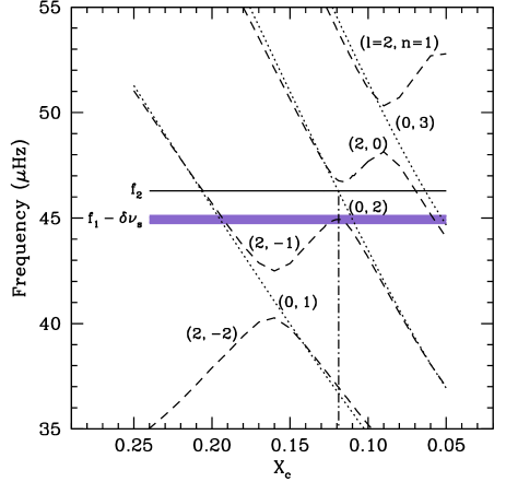
The clue to our problem lies in recognising the fact that such a small (but not too small) difference between the $\ell=0$ and $\ell=2$ modes can only occur in case of an avoided crossing. As long as the modes follow the regular smooth separation patterns, we will never find a solution where the $\ell=0$ and $\ell=2$ modes have the appropriate separation as required by the observations. This is illustrated in Fig. 5. In this figure, we show how the $\ell=0$ and $\ell=2$ modes vary with evolution of a given star. For the purpose of illustration, we have assumed an average value of the rotational splitting (with an error margin) and corrected the observed frequency, $f_{1}$, to compare it with the theoretical frequency. As the star evolves, the density gradient at the edge of the shrinking convective core increases. This has the effect of rapidly increasing the frequencies of the $g$-modes, which causes successive “bumping” of the modes. For example, as shown in Fig. 5, the $g_{2}$ mode of the $\ell=2$ degree first increases (for $X_{\mathrm{c}}\geq 0.16$), until it bumps into the $g_{1}$ mode (around $X_{\mathrm{c}}\simeq 0.16$), creating an avoided crossing between these two modes at that age. With further evolution, the $g_{1}$ mode increases in value until it creates another avoided crossing with the $f$-mode (around $X_{\mathrm{c}}\simeq 0.12$). Progressively, higher order modes are bumped as the star evolves. An excellent discussion of such mode bumping is provided by Aizenman et al. (1977).

We find that as long as we are constrained by the position of $\beta$ CMa on the HR diagram, the required separation between the $\ell=0$ and $\ell=2$ modes ($\sim 1.2\leavevmode\nobreak\ \mu\mathrm{Hz}$ around a frequency value of $45\leavevmode\nobreak\ \mu\mathrm{Hz}$) cannot be obtained if the radial mode is the fundamental mode. Even for an avoided crossing, the appropriate separation between the radial fundamental and the $\ell=2,n=-2$ bumped up mode occurs at a much lower frequency than observed. Fig. 5, which represents a typical model at the appropriate position on the HR diagram, confirms this. However, a solution is indeed plausible if we consider the observed radial mode to be the first overtone instead. In that case, the avoided crossing between the $\ell=2$ $g_{1}$ and $f$-modes bumps the $g_{1}$ close to the $\ell=0,n=2$ mode. We now, therefore, explore the possibility of the radial mode being the first overtone mode.

By considering the radial mode as the first overtone ($\ell=0,n=2$), we do indeed find a number of models with different stellar parameters that match the observed frequencies. Specifically, $f_{2}$ is matched with the $\ell=0,n=2$ mode, and $f_{1}$ with the $\ell=2,n=-1$ mode, after correcting for the rotational splitting. We have also checked the excitation rates of these two frequencies by the nonadiabatic oscillation code, MAD (Dupret 2001) and found both of them to be excited for all the models which fit the data.

Figure 6: The variation of the model frequencies with three stellar parameters – $M$, $d_{\mathrm{ov}}$ and $Z_{0}$ – are shown. In each panel, two of the parameters are fixed to clearly bring out the effect of the remaining parameter on the frequencies. The $\ell=0,n=2$ frequencies are plotted as abcissae, while the $\ell=2,n=-1$ frequency, corrected for rotational splitting, are plotted as ordinates. The dashed lines indicate the two observed frequencies. The point where the two dashed lines intersect indicate the perfect match of the desired model. Each shaded band represents an evolutionary track. The width of the band along the $y$-axis indicates the uncertainty due to the rotational splitting. A full-colour version of this figure is available in the online edition.

A similar solution with the radial mode being the second overtone ($\ell=0,n=3$) and the $\ell=2$ mode being the bumped-up $f$-mode is again ruled out because the relevant avoided crossing occurs at a higher frequency than observed.

The common feature of all the possible solutions is the fact that the $\ell=2,n=-1$ mode is an avoided crossing with the $f$-mode. This helps to constrain the stellar parameters a great deal, especially the age (or $X_{\mathrm{c}}$) of the model. The requirement that the star must be at the precise age for a specific avoided crossing to occur, is indeed a very strict one. Nevertheless, since we have only two frequencies to constrain our model with, we do find multiple combinations of the stellar parameters where such a solution exists. We have investigated the limits of the stellar parameters that can be constrained with the observed frequencies (see next section). Although the limits on effective temperature and luminosity were not explicitly used in determining the best models, all of them do lie well within the errorbox on the HR diagram adopted in Sect. 3.1.

3.6 Limits on stellar parameters

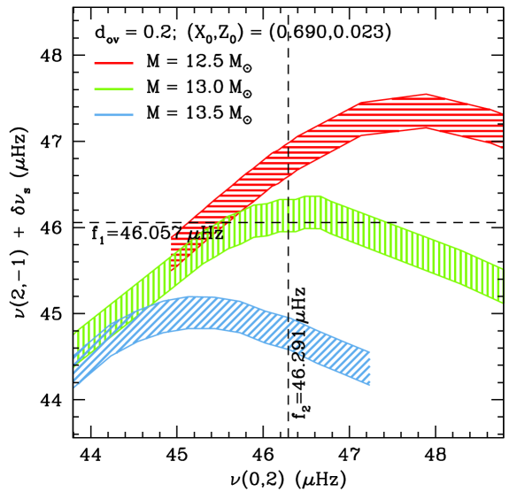
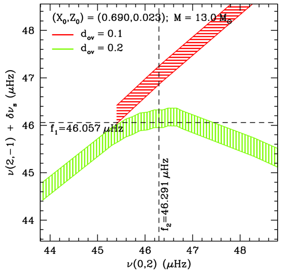
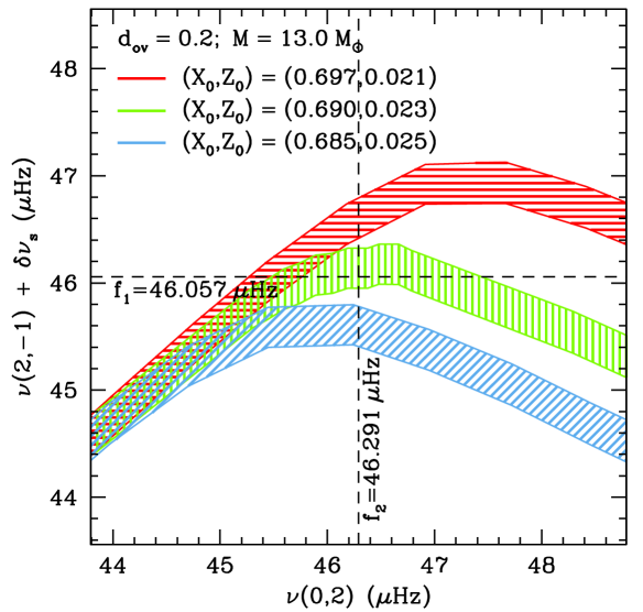
We have, in principle, four major stellar parameters to tune our models with – $M$, $d_{\mathrm{ov}}$, $X_{0}$ and $Z_{0}$. For each appropriate combination of these parameters, the age (in terms of $X_{\mathrm{c}}$) is automatically chosen by the closest match of the frequencies. The initial hydrogen abundance, $X_{0}$, must, however, be linked somewhat to the metallicity, $Z_{0}$; we have varied $X_{0}$ only within permissible limits for a particular choice of $Z_{0}$ so that $\mathrm{[M/H]}$ remains within the bounds quoted in Sect. 3.1. In Fig. 6, we have shown how the relevant frequencies of the models, $\nu(\ell=0,n=2)$ and $\nu(\ell=2,n=-1)$, vary as each of the stellar parameters are changed. In each panel, only one parameter is changed at a time, keeping the others constant. Each band is, in fact, an evolutionary track – the sense of evolution being from the right to the left (decreasing radial frequency). The width of the shaded bands along the $y$-axis reflects the uncertainty due to the rotational splitting correction. The tracks are truncated beyond the ages where the models lie outside the error box on the HR diagram. Our best models lie near the centre of each plot, where both the model frequencies match the observed ones.

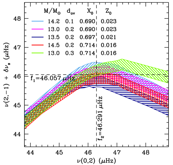
In Fig. 7 we vary multiple parameters simultaneously to obtain a good match of the model frequencies with the observed ones. This illustrates that several solutions are possible in the multi-dimensional parameter space. Actually, we have shown only the models with the extreme limits of the stellar parameters for which a solution can still be found. These are only indicative of the trend of the frequencies of the models, and several other solutions are possible when the parameters (especially overshoot and metallicity) are varied within their bounds. Table 3 lists the physical parameters for these selected models.

We find that no solutions are possible in the absence of core overshoot. Even with a small amount of overshoot ($d_{\mathrm{ov}}=0.1$), we need to have a higher mass to obtain a solution. The higher stellar mass helps to increase the mass of the convective core to offset the low overshoot. Most of our best fit models use $d_{\mathrm{ov}}=0.2$. Higher overshoot ($d_{\mathrm{ov}}=0.3$) models can reproduce the frequencies only for low metallicity and proportionally lower helium content, again suggesting a trade-off between overshoot and helium content to maintain a balance of the core size. This indicates that the size of the convective core plays a crucial role in determining the frequencies. Indeed, all our best fit models, including those with low and high overshoot have fractional convective core mass of $24$–$28\%$.

Table 3: Physical parameters of representative stellar models that match the observed frequencies.

$M/M_{\odot}$	$X_{\mathrm{c}}$	$X_{0}$	$Z_{0}$	$d_{\mathrm{ov}}$	$\log T_{\mathrm{eff}}$	$\log L/L_{\odot}$	$R/R_{\odot}$	Age(Myr)
14.2	0.105	0.690	0.023	0.1	4.378	4.530	10.67	10.95
13.0	0.127	0.690	0.023	0.2	4.364	4.440	10.35	13.04
13.5	0.128	0.697	0.021	0.2	4.373	4.488	10.50	12.48
14.5	0.123	0.714	0.016	0.2	4.391	4.582	10.75	11.75
13.0	0.134	0.714	0.016	0.3	4.370	4.471	10.40	14.49

The mass of our best fit models are mostly limited to $13.5\pm 0.5M_{\odot}$, for $d_{\mathrm{ov}}=0.2$. The mass could be higher (up to $14.5M_{\odot}$) if either the metallicity is low ($\mathrm{[M/H]}=-0.06$) or the overshoot is low ($d_{\mathrm{ov}}=0.1$). The central hydrogen abundance of the best models are limited to the range $0.128\geq X_{\mathrm{c}}\geq 0.123$, for overshoot values of $d_{\mathrm{ov}}=0.2$. As expected, the low overshoot models have younger ages and lower $X_{\mathrm{c}}$. The situation is opposite for high overshoot models.

Figure 7: Similar to Fig. 6, except that multiple parameters are varied at a time to obtain a good match between the theoretical frequencies and the observed ones. Selected models with limiting values of overshoot and metallicity are shown only. A full-colour version of this figure is available in the online edition.

4 Conclusions

$\beta$ Canis Majoris is one of the $\beta$ Cephei stars whose variability has been observed and analysed for one century. It was discovered that this star pulsates with three frequencies rather low in comparison with other known stars of its type. For this reason $\beta$ CMa is an important target for asteroseismology purposes. However, so far, no definite mode identification had been achieved for this star so that no modelling could be attempted. Our aim was to increase the number of known pulsating frequencies and mostly to provide a unique identification of the modes of $\beta$ CMa.

Our study was based on 452 ground-based high-resolution high S/N spectroscopic measurements spread over 4.5 years. We used the Si III 4553 Å line to derive the pulsation characteristics of $\beta$ CMa. Our dataset unfortunately suffers from strong aliasing but the three established frequencies of the star were confirmed in the first three velocity moments of the line and in the spectra themselves. They are $f_{1}=3.9793\leavevmode\nobreak\ \mathrm{c\,d}^{-1}$ ($f_{1}=46.057\leavevmode\nobreak\ \mu\mathrm{Hz}$), $f_{2}=3.9995\leavevmode\nobreak\ \mathrm{c\,d}^{-1}$ ($f_{2}=46.291\leavevmode\nobreak\ \mu\mathrm{Hz}$) and $f_{3}=4.1832\leavevmode\nobreak\ \mathrm{c\,d}^{-1}$ ($f_{3}=48.417\leavevmode\nobreak\ \mu\mathrm{Hz}$). Unfortunately no new frequencies were discovered neither in our spectroscopic observations nor in the recent multisite photometric measurements led by Shobbrook et al. (2006).

The important result of the combination of both intensive campaigns is an identification of the two main modes of $\beta$ CMa, which is a strong constraint for further asteroseismic modelling of the star. The photometric identification by Shobbrook et al. (2006) yielded $\ell_{1}=2$ and $\ell_{2}=0$. Our spectroscopic data could corroborate that the mode with $f_{2}$ is radial. We adopted the photometric identification of $\ell_{1}$ and spectroscopic techniques allowed us to derive the $m$-value of the main mode. The application of the moment method gave a preference to $m_{1}=2$. Because moment solutions could not definitely exclude $m_{1}=1$ we made use of the behaviour of the amplitude distributions across the line profile for the best parameter sets given by the moment method. In this way we could conclude without any doubt that $(\ell_{1},m_{1})=(2,2)$. For the third mode nothing could be concluded. In addition we derived a stellar equatorial rotational velocity of $31\pm 5\mathrm{km\,s}^{-1}$.

The definite identification of two of the observed modes and a much improved estimate of the rotation velocity of $\beta$ CMa allowed us to attempt the first seismic modelling of this star. Although it is not realistic to hope for a unique model to fit just two frequencies, we have thoroughly explored the stellar parameter space to derive reasonable constraints for the mass, age, and core overshoot. The most significant aspect of the seismic analysis is the fact that we could assert that the non-radial mode, $f_{1}$, is close to an avoided crossing. This implies a very strong constraint on the stellar parameters, especially the age of the star. At the same time, it rules out the possibility of the radial mode, $f_{2}$, being the fundamental mode. This makes $\beta$ CMa one more $\beta$ Cephei star known to have a dominant radial overtone mode of pulsation (cf. Aerts et al. 2006).

Our best fit models indicate that $\beta$ CMa has a mass of $13.5\pm 0.5M_{\odot}$, an age of $12.4\pm 0.7$ Myr ($X_{\mathrm{c}}=0.126\pm 0.003$) and core overshoot of $d_{\mathrm{ov}}=0.20\pm 0.05$. No satisfactory model can be found if core overshoot is absent. A small overshoot parameter is possible only for a higher mass along with high metallicity (and proportionally higher helium content). On the other hand, higher core overshoot is required if the star is metal-poor ($\mathrm{[M/H]}<-0.05$). However, Morel et al. (2006) found the composition of $\beta$ CMa not much different from that of the Sun, making such possibilities unlikely. Therefore, it is safe to conclude that the models with $d_{\mathrm{ov}}=0.20\pm 0.05$ are the most likely ones. If the chemical composition of $\beta$ CMa could be known to higher accuracy independently, one would be able to constrain the other parameters even more. All the solutions turn out to have effective temperatures close to the cooler edge of the adopted errorbox on the HR diagram. This is consistent with the recent estimates of $T_{\mathrm{eff}}$ (e.g., Morel et al. 2006). We note that we had deliberately chosen a very conservative errorbox for effective temperature and luminosity; a stricter limit on these parameters would rule out some of our possible models.

In retrospect, one can also try to identify the mode of oscillation for the third frequency, $f_{3}$, by comparing it with the theoretical model frequencies. In this comparison, we allowed for different rotational splitting values, $m_{3}$, for each non-radial mode with the restriction $m_{3}>0$, as we found in Sect. 2. This leads us to only one possibility for $f_{3}$, for all the models which match $f_{1}$ and $f_{2}$: $\ell_{3}=3,m_{3}=2,n_{3}=-1$. We hope that this identification of $f_{3}$ can be checked through future observations. However, we cannot place further constraints on the models at this stage using this frequency; all the models with stellar parameters in the range restricted by the first two frequencies also match the third frequency with the identification given above within the uncertainty associated with the rotational velocity. One would need a more precise estimate of the rotational velocity to distinguish between these models.

The rotation period may be calculated from our estimate of the equatorial velocity (Sect. 2.4) and the radius of our best models which indeed lie in a narrow range (Table 3). We estimate the rotation period to be $18.6\pm 3.3$ days, which indicates that $\beta$ CMa is indeed a slow rotator; therefore, our assumption in neglecting higher order terms of the rotation velocity while calculating the frequency splitting stands justified.

Despite the knowledge of only two frequencies for this star, the occurrence of the avoided crossing goes a long way towards constraining most of the stellar parameters. While one cannot expect to be so lucky for every star, we have shown that the identification of an avoided crossing might help us to extract a lot more information about the star than any normal mode.