30 Glitches in slow pulsars

We have analyzed 5.5 years of timing observations of 7 “slowly” rotating radio pulsars, made with the Westerbork Synthesis Radio Telescope. We present improved timing solutions and 30, mostly small, new glitches. Particularly interesting are our results on PSR J1814$-$1744, which is one of the pulsars with similar rotation parameters and magnetic field strength to the Anomalous X-ray Pulsars (AXPs). Although the high-B radio pulsars do not show X-ray emission, and no radio emission is detected for AXPs, the roughly similar glitch parameters provide us with another tool to compare these classes of neutron stars. Furthermore, we were able to detect glitches one to two orders of magnitude smaller than before, for example in our well-sampled observations of PSR B0355$+$54. We double the total number of known glitches in PSR B1737$-$30, and improve statistics on glitch sizes for this pulsar individually and pulsars in general. We detect no significant variations in dispersion measure for PSRs B1951$+$32 and B2224$+$65, two pulsars located in high-density surroundings. We discuss the effect of small glitches on timing noise, and show it is possible to resolve timing-noise looking structures in the residuals of PSR B1951$+$32 by using a set of small glitches.

1 Introduction

Two sorts of irregularities, in the otherwise very stable pulsar rotation rates exist, which limit the accuracy to which pulse arrival times can be measured: timing noise and glitches.
Timing noise is seen as random fluctuations in the rotation rate of the pulsar on timescales of days to years. It is largest in young pulsars and pulsars with large period derivatives (Cordes & Helfand 1980; Arzoumanian et al. 1994).

Glitches on the other hand are characterized by a sudden increase of the pulsar rotation frequency $(\nu)$, accompanied by a change in spindown rate $(\dot{\nu})$ and sometimes followed by relaxation or exponential decay to the previous rotation state. Typical magnitudes of glitches are from $10^{-10}\nu$ to $10^{-6}\nu$ and steps in slowdown rate are on the order of $10^{-3}\dot{\nu}$. Glitches give an unique opportunity to study the internal structure of neutron stars, as they are believed to be caused by sudden and irregular transfer of angular momentum from the superfluid inner parts of the star to the more slowly rotating crust (Ruderman et al. 1998). They are mostly seen in pulsars with characteristic ages ($\tau_{c}$) around $10^{4}-10^{5}$ yr and can occur up to yearly in some pulsars. Most of the youngest pulsars, with $\tau_{c}\lesssim 2000$ yr show very little glitch activity. This could be because they are still too hot which allows the transfer of angular momentum to happen more smoothly (McKenna & Lyne 1990).

A lot of new glitches have been found in the last decades (Lyne et al. 2000; Urama & Okeke 1999; Wang et al. 2000). This makes statistical analysis of glitch sizes and activity possible. However, no clear relations between glitch parameters or dependence of glitch parameters on rotation properties have been found so far. Extending the sample of glitches, especially with previously unknown small-magnitude glitches will lead to a better insight into the glitch mechanism and the structure of the neutron star.

2 Observations and data analysis

We have observed our sample of pulsars since 1999 at the Westerbork Synthesis Radio Telescope (WSRT) with the Pulsar Machine (PuMa; Voûte et al. 2002). Depending on brightness, we observed each pulsar at multiple frequencies centered at 328, 382, 840 or 1380 MHz as shown in Table 1. We have approximately monthly observations of 6 to 60 minutes duration. The sampling time for all observations was 0.4096 ms and the bandwidth used was 8$\times$10 MHz for the observations at 840 and 1380 MHz. The low-frequency observations only used 10 MHz of bandwidth, and were usually simultaneous at both frequencies. Each 10 MHz band was split into 64 channels.

The data was dedispersed and folded offline, and then integrated over frequency and time over the whole duration to get a single profile for each observation. The profile was cross-correlated with a standard profile, obtained from the summation of high signal-to-noise (S/N) profiles, to calculate a time of arrival (TOA) for each observation. These were referred to local time using time stamps from a H-maser at WSRT. These times are converted to UTC using GPS maser offset values measured at the observatory, and clock offsets from the IERS. The times of arrival were converted to the Solar system barycentre using the JPL ephemeris DE200 (Standish 1982).

The TOAs are analysed with TEMPO (version 11.002), using a model including position, rotation frequency, first derivative and dispersion measure (DM) of the pulsar. In this version of TEMPO it was only possible to fit for the parameters of 4 different glitches simultaneously. Because of the large numbers of glitches we found, in for example PSR B1737$-$30, it was necessary to be able to fit for more glitches, so we extended the number of glitch parameters to enable fitting up to 9 glitches simultaneously.

A glitch can be recognized by the sudden increase of the rotation frequency, causing the residuals from the timing model to increase towards earlier arrival (e.g. Figs. 1 and 2). Glitches can be described as combinations of steps in rotational frequency and its derivative, of which parts can decay exponentially on various timescales. Usually only the larger glitches show measurable exponential decay. Because we mostly found small-magnitude glitches, we could only fit for the permanent steps in frequency and frequency first derivative. The few large glitches we found in PSR B1737$-$30 were not sufficiently well sampled to enable us to fit the exponential decay, or a new glitch happened too soon after a large one which caused the relaxation part, if present, to be absorbed in the next glitch parameters.

Solutions before and after the glitch epoch are used to roughly estimate the steps in frequency and its first derivative. If the gap between observations around the glitch epoch is not too large, the epoch can be found more accurately by requiring a phase-connected solution over the gap. This is done using another parameter in TEMPO, GLPH, which represents a fraction of the phase needed as a jump to get a connected solution. Minimization of this parameter by changing the epoch results in the best value for the glitch epoch. However if the gap is too large, rotations can be missed and the glitch epoch is estimated as the mid-point of the gap.

Table 1: Summary of observed frequencies.

Pulsar Name	328 MHz	382 MHz	840 MHz	1380 MHz
B0355$+$54	$\star$	$\star$	$\star$	$\star$
B0525$+$21	$\star$	$\star$	$\star$	$\star$
B0740$-$28	$\star$	$\star$	$\star$	$\star$
B1737$-$30			$\star$	$\star$
J1814$-$1744				$\star$
B1951$+$32			$\star$	$\star$
B2224$+$65			$\star$	$\star$

3 Individual pulsars: Results

Table 2: Position and rotation parameters. The uncertainties are the standard TEMPO errors and refer to the last digit quoted. Rms values result from models including glitch parameters presented in Table 3.

Pulsar name	B0355$+$54	B0525$+$21	B0740$-$28
	J0358$+$5413	J0528$+$2200	J0742$-$2822
Right ascension (J2000)	03:58:53.7166(3)	05:28:52.26(1)	07:42:49.082(3)
Declination (J2000)	54:13:13.717(3)	22:00:03(3)	$-$28:22:43.96(6)
Epoch (MJD)	52350	52362	52200
Data span (MJD)	51386$-$53546	51408$-$53548	51386$-$53546
Frequency $\nu$ (s-1)	6.39453829911(4)	0.26698470619(3)	5.996409260(2)
Frequency first derivative $\dot{\nu}$ ($10^{-15}$ s-2)	$-$179.747(1)	$-$2.8537(3)	$-$604.71(4)
Frequency second derivative $\ddot{\nu}$ ($10^{-24}$ s-3)	0.18(2)		0.9(1)
Dispersion measure $DM$ (pc cm-3)	57.1420(3)	50.87(1)	73.782(2)
Characteristic age $\tau_{c}$ (kyr)	564	1480	157
Surface magnetic field strength $B$ ($10^{12}$G)	0.84	12.4	1.69
Glitch activity $A_{g}$ ($10^{-7}$ yr-1)	0.0004	0.003	0.01
Number of TOAs	184	83	209
Rms timing residual ($\mu$s)	47	777	709

	B1737$-$30		B1951$+$32	B2224$+$65
	J1740$-$3015	J1814$-$1744	J1952$+$3252	J2225$+$6535
Right ascension (J2000)	17:40:33.75	18:14:43.10(5)	19:52:58.164(5)	22:25:52.627(3)
Declination (J2000)	$-$30:15:43.8	$-$17:44:48(8)	32:52:40.38(5)	65:35:35.16(2)
Epoch (MJD)	52200	52353	52245	52400
Data span (MJD)	51427$-$53100	51391$-$53545	51427$-$53546	51427$-$53546
Frequency $\nu$ (s-1)	1.6480330270(4)	0.251515052(1)	25.29570396(1)	1.4651138511(2)
Frequency first derivative $\dot{\nu}$ ($10^{-15}$ s-2)	$-$1266.635(7)	$-$47.11(2)	$-$3737.3(4)	$-$20.774(3)
Frequency second derivative $\ddot{\nu}$ ($10^{-24}$ s-3)			54(8)	$-$0.55(3)
Dispersion measure $DM$ (pc cm-3)	152.15(2)	830	45.19(2)	36.42(2)
Proper motion in right ascension (mas yr-1)				106(15)
Proper motion in declination (mas yr-1)				174(18)
Characteristic age $\tau_{c}$ (kyr)	21	85	107	1118
Surface magnetic field strength $B$ (1012G)	17	55	0.49	2.6
Glitch activity $A_{g}$ ($10^{-7}$ yr-1)	1.6	0.08	0.008	0.0007
Number of TOAs	64	80	106	97
Rms timing residual ($\mu$s)	150	8580	359	215

3.1 PSR B0355$+$54 (J0358+5413)

This relatively old pulsar ($5.6\times 10^{5}$ yr) has been studied intensively since its discovery (Manchester et al. 1972). It has low timing noise and the only report of glitches in this pulsar is by Lyne (1987) and Shabanova (1990). The reported glitches are very different, the first happened at MJD 46079 and was quite small with $\Delta\nu/\nu=5.6\times 10^{-9}$. The second, at MJD 46496, is one of the largest glitches known, with $\Delta\nu/\nu=4.4\times 10^{-6}$.

We have a well-sampled multi-frequency observing data span of almost 6 years for this pulsar. We improve on previously published (Hobbs et al. 2004; Wang et al. 2001) timing solutions. Although a timing solution for our data span including only position parameters and two frequency derivatives already yields a better root-mean-square (rms) of 67 $\mu s$, we find a better solution (47 $\mu s$) including 4 mini-glitches with frequency steps over an order of magnitude smaller than any glitch found to date in a slowly rotating pulsar: $\Delta\nu/\nu$ of $10^{-10}$ to $10^{-11}$. In Fig. 1 the residuals with and without fitting for these glitches are shown. The upper plots show the result for keeping all parameters fixed but leaving the glitches out one at the time, the bottom plot shows the best-fit solution to our data including the four mini-glitches. Parameters for this solution can be found in Tables 2 and 3.

Because these mini-glitches are so much smaller than any glitch found before, we investigated what our detection limit is for glitches in this pulsar by carrying out simulations. We first created a set of times of arrival resembling a model including a mini-glitch. This was done by fitting our data set to the model, but keeping all, including the simulated glitch parameters, fixed. The resulting residuals were used to correct all individual TOAs so that they would follow the model exactly. Then random noise was added to each TOA with a level typical for this pulsar. These new TOAs were used in the usual process of finding a timing solution to see whether we could significantly redetect the glitch. For this pulsar, the simulations have shown that we can detect glitches as small as $\Delta\nu/\nu=10^{-11}$.

Figure 1: Detection of four miniglitches in PSR B0355$+$54. a) Residuals when not fitting for any glitches and keeping best-solution rotation and position parameters fixed (Table 2). The epochs of the glitches are indicated by arrows in the upper plot. The residuals bend down to earlier arrival at the epoch of the first glitch (MJD 51673). b) Like plot (a), but also including the parameters for the first glitch; the residuals bend down at the epoch of the second glitch (MJD 51965). c) Third glitch (MJD 52941). d) Fourth glitch (MJD 53216). Plot (e) shows the residuals for our best-fit model, including the four mini-glitches (Table 3).

3.2 PSR B0525$+$21 (J0528+2200)

Only one small glitch has been observed before in this old, very slowly rotating pulsar (Downs 1982; Shemar & Lyne 1996). It occurred at MJD 42057 and had a magnitude of $\Delta\nu/\nu=1.2\times\leavevmode\nobreak\ 10^{-9}$. An exponential decay of 50% in 150 days was measured.

We find a glitch at MJD 52284 with similar parameters as the one before, with a magnitude of $\Delta\nu/\nu=1.46\times\leavevmode\nobreak\ 10^{-9}$. Unfortunately the new glitch occurs in a large gap in our data span which makes it impossible to fit for an exponentional decay. Our data suggests that another glitch happened around MJD 53375 (January 2005). When using data up until June 2005, we can only fit for the step in frequency, which appears to be small, $\Delta\nu/\nu=1.7\times\leavevmode\nobreak\ 10^{-10}$.

3.3 PSR B0740$-$28 (J0740-2822)

D’Alessandro et al. (1993) have reported two small glitches in this pulsar, at MJDs 47678 and 48349 with relative sizes 2.63 and 1.5 $\times\leavevmode\nobreak\ 10^{-9}$. Another two small glitches (1.9 and 1.3 $\times\leavevmode\nobreak\ 10^{-9}$) at MJDs 49298 and 50376 were reported by Urama & Okeke (1999).

With the four new glitches we find, this pulsar is showing regular glitching behaviour, with small glitches roughly every 900 days. All glitches are surprisingly similar in magnitude.

3.4 PSR B1737$-$30 (J1740-3015)

This frequently glitching pulsar has been intensively studied since 1987 by McKenna & Lyne (1990), Shemar & Lyne (1996), Urama & Okeke (1999) and Krawczyk et al. (2003). It has a large spindown value of $-1.267\times\leavevmode\nobreak\ 10^{-12}$ s^-2. Large glitches, with magnitudes $\Delta\nu/\nu$$\approx$$10^{-7}$, occur roughly every 800 days, and smaller ones every 2–300 days. Fourteen glitches have been reported up to MJD 51000.

Because of the large number of glitches in a short time, and the location of the pulsar close to the ecliptic plane, it is difficult to find a good value for the pulsar declination in the timing solution. Therefore we first use a recently published value for the position, from Wang et al. (2001), and keep this position fixed when fitting for the glitches.

Due to a limited number of data points in the middle of our data set, we were at first not able to find a connected timing solution. In overlap with our data span, five glitches were reported in the conference proceedings of the Lake Hanas Pulsar meeting (2005) by Esamdin et al. and Zou et al. We used the glitch parameters they found to create a phase-connected solution for our data set covering almost 4.5 years.

We find a solution confirming those glitches and add 5 new small ones, which results in a continuing high glitch rate of $10$ new glitches in 4.5 years for this pulsar. Some of those are an order of magnitude smaller than the smallest glitch found before for this pulsar.

We almost double the total number of glitches known for this pulsar. This allows us to have better statistics on the glitch size distribution. In the bottom panel of Fig. 4 a histogram of glitch sizes is shown, including all known glitches for PSR B1737$-$30. With the new, mostly small glitches included, the sizes appear to be roughly equally distributed between $\Delta\nu/\nu=10^{-10}$ and $10^{-6}$.

3.5 PSR J1814$-$1744

This pulsar was discovered in 1997 (Camilo et al. 2000). Its estimated surface dipole magnetic field strength is one of the highest known for radio pulsars, $5.5\times\leavevmode\nobreak\ 10^{13}$G. This is very close to the magnetic field strengths for anomalous X-ray pulsars (AXPs). The spin parameters are very similar as well. However, no X-ray emission was detected for this pulsar (Pivovaroff et al. 2000). There are now six high-B radio pulsars known. Two have been detected in X-rays, but all have X-ray luminosity upper limits one to three orders of magnitudes less than AXPs (Pivovaroff et al. 2000; McLaughlin et al. 2003; Gonzalez et al. 2004; Kaspi & McLaughlin 2005).

Three glitches have been detected in AXPs so far: two in 1RXS J1708$-$4009, and one in 1E 2259$+$586. In Table 4 the glitches found for all high-magnetic field objects are shown. The steps in frequency in AXP glitches seem at least an order of magnitude larger than those in the high-B radio pulsars, but the values are not uncommon for radio pulsars in general. For example the Vela pulsar and PSR B1737$-$30 show comparably large-magnitude glitches.

We have detected three glitches for PSR J1814$-$1744. The parameters are listed in Table 3 and the residuals are shown in Fig. 2. Together with another glitch detected in the high-magnetic field pulsar J1119$-$6127 (Camilo et al. 2000), we are now able to compare AXPs and radio pulsars in another way.

Figure 2: Glitch detections in PSR J1814$-$1744. Like Fig. 1, the upper plots (a,b,c) show the residuals for the best-fit model and including parameters for each glitch in turn for each following plot. The second, larger glitch is already clearly visible in plot (a). Plot (d) shows the residuals for the best-fit model including the parameters for the three glitches detected.

3.6 PSR B1951$+$32 (J1952+3252)

This low-magnetic field pulsar was discovered in 1987 by Kulkarni et al. (1988), and is associated with the CTB 80 supernova remnant (Strom 1987). Timing solutions have been presented by Foster et al. (1994) and Hobbs et al. (2004). A small glitch was detected by Foster et al. (1990) in the beginning of March 1988.

Because of the high timing activity of this pulsar, it was quite difficult to find a new timing solution for this pulsar when starting from a solution with an epoch just before the start of our data span. Only by shifting the epoch a few hundred days at a time and creating new solutions for each next epoch could we generate the present solution with the epoch in the middle of our data set.

We found a solution for our data span of 5.5 years consisting of observations at 840 and 1380 MHz. The solution has a rms of 3.2 ms, which is the best timing solution so far found for this pulsar only including the first two frequency derivatives. The residuals show a large timing activity, see Fig. 3-a. We noticed that the $\ddot{\nu}$ was surprisingly stable when fitting for small parts of the data, therefore we also included a third derivative in our solution. This results in a better solution (2.2 ms) than the one using only two frequency derivatives, but still a lot of timing activity is present (Fig. 3-b).

The pulsar is currently interacting with its supernova remnant, and has a high proper motion (Hobbs et al. 2005). Therefore it is not unlikely that DM variations are influencing our timing solution. To get a better view of the influence of the medium surrounding the pulsar on the arrival times, we searched for dispersion measure variations in our data set. Starting from the solution including only position and rotation parameters, we fixed all parameters and fitted only for DM over small parts of the data set. The result can be seen in Fig. 4. Although our errors are too large to constrain the variations, the DM appears to be wandering slowly around the mean value of $45.19$ pc cm^-3, but no clear trend is seen. This indicates that DM variations are not responsible for the timing-noise in this pulsar.

The pulsar has shown glitching behaviour before, and the cusp-like structures in the residuals are known to be an indication for glitches (Hobbs 2002). Therefore we tried to resolve the variations with glitches.

A solution including four glitches results in a much better rms of 0.4 ms for our data span. The glitches we use are of similar magnitude to the one reported by Foster et al. (1990). The steps in frequency derivative are also comparable, see Table 3. The residuals are shown in Fig. 3-c. Another glitch is likely to have happened around MJD 51500, at the beginning of our observing span. Because we have only three data points before that date, which prevents us from sampling the rotation properties properly, we have excluded them.

Figure 3: PSR B1951+32: a) Residuals to a model including two frequency derivatives. b) Residuals for a timing solution also including a third frequency derivative. c) Residuals for the solution presented in Tables 2 and 3. Note that the vertical scale is $10$ times smaller than plots (a) and (b). For all diagrams, circles are observations at 1380 MHz, squares at 840 MHz.

Figure 4: DM measurements for PSR B1951+32. Each point is calculated using two observations at 1380 MHz, and two observations at 840 MHz. For each point, we fit for DM keeping the parameters for the solution presented in Fig. 3-a fixed. The horizontal line represents the average DM found for the best timing solution.

3.7 PSR B2224$+$65 (J2225+6535)

For this old pulsar only one glitch has been found before, by Backus et al. (1982). It was very large, with a magnitude of $\Delta\nu/\nu\approx 1.7\times 10^{-6}$. An upper limit of $\Delta\dot{\nu}/\dot{\nu}=0.003$ on the step in frequency derivative was given. Shemar & Lyne (1996) used improved rotation parameters to confirm the glitch parameters, and they also report a $\ddot{\nu}$ of $0.1\times 10^{-24}$s^-3.

We report three very small new glitches for this pulsar, with steps in rotation frequency of $\Delta\nu/\nu$ of $0.14,0.08$, and $0.19\leavevmode\nobreak\ \times\leavevmode\nobreak\ 10^{-9}$ respectively (Table 3).

PSR B2224$+$65 is traveling at very high speed in the Guitar Nebula. Chatterjee & Cordes (2004) report on shape evolution of the tip of the nebula, where the pulsar is located: ”the observations reflect the motion of the pulsar through random density inhomogeneities combined with a gradient toward a region of lower density.”

Like for PSR B1951$+$32, we have searched our data for dispersion measure variations. The result is shown in Fig. 5. Our data is consistent with a stable dispersion measure. However, we have insufficient sensitivity to measure the very small variations predicted by Chatterjee & Cordes (2004).

Figure 5: DM variations for PSR B2224+65. Crosses: each point is calculated using two observations at 1380 MHz, and two observations at 840 MHz. Squares: each point is calculated using all data points in intervals of 200 days. Horizontal line is the average DM value for the best timing solution.

4 Discussion

4.1 Glitch sizes

Little is known about the range of glitch sizes and their distribution within this range. Lyne et al. (2000) showed a distribution for 48 glitches in 18 pulsars. They claimed there was a peak around $\Delta\nu/\nu\approx 10^{-6.5}$, but they also noted that the glitch sample could be incomplete at the lowest level. How small do we expect glitches to be? Glitches are believed to be the result of the unpinning of neutron superfluid vortices which causes transfer of angular momentum of the interior superfluid to the solid crust of the star. There is no report of restrictions on a minimum stress needed before vortices unpin, so it is not unlikely that the observed lower limit on glitch sizes is mainly due to the detection limits of the observing systems and the timing precision achievable for a given pulsar.

In this paper we measure glitch sizes down to $\Delta\nu/\nu=10^{-11}$, which provides the first evidence that such small glitches occur and can be measured in slowly rotating pulsars. These glitches are then of a similar size to the one reported by Cognard & Backer (2004) in a millisecond pulsar, and thus perhaps provide further evidence for a continuous distribution of glitch sizes.

Let us now consider how these small glitches affect the observed glitch size distribution. In Fig. 4, a histogram is shown for all now known glitch sizes. New glitches found in this study are shown added on top of the old glitch distribution. A Kolmogorov-Smirnov test shows that over the whole range, the distribution has only a probability of $0.001$% to be consistent with a flat distribution in log space of glitch sizes. But if we consider only the part of the diagram between $10^{-9}\leavevmode\nobreak\ <\leavevmode\nobreak\ \Delta\nu/\nu\leavevmode\nobreak\ <\leavevmode\nobreak\ 10^{-5.5}$, where the statistics are better, another KS test shows that the distribution has a $29.8$% chance to be drawn from a flat distribution. The increased number of glitches with sizes around $\Delta\nu/\nu\approx 10^{-9}$, now comparable to the amount of larger glitches observed, suggests again that the lack of the smallest glitches at the lower end of the distribution is due to observing limits. The lack of glitches at the upper end of the distribution can not be due to observing limits. Apparently there is some physical restriction to the maximum size of a glitch, and we can consider the boundary of $\Delta\nu/\nu\approx 10^{-5}$ as the natural upper limit of glitch sizes.

The glitch size distribution may be biased because there is a whole range of different pulsars included, which can all show different glitching behaviour. For example the Vela pulsar suffers from a large number of huge glitches. The fact that those are more easily detectable, will have a large influence on the overall glitch size distribution. We take a frequently glitching pulsar, PSR B1737$-$30 and make a similar histogram as before to see what happens if we study the glitch size distribution for one pulsar. The result is shown in the bottom panel of Fig. 4. As we now have almost doubled the number of glitches detected for this pulsar, and we measure glitches an order of magnitude smaller than before, we can do a statistical analysis of the glitch size distribution for a single pulsar with glitches covering almost the whole range of sizes observed. Using a Kolmogorov-Smirnov test, we calculated that in the observed size range there is a $90.2$% probability that the glitches of PSR B1737$-$30 are drawn from a flat distribution (in log space) of glitch sizes.

The greater glitch rate of PSR B1737$-$30 allows us to obtain sufficient glitches to show that the distribution of glitches in this pulsar are likely drawn from a flat log-space distribution of glitch sizes. Whether this is representative of the glitch size distribution of pulsars in general is more difficult to determine based on just this pulsar and a larger sample of pulsars where such fits can be determined is required.

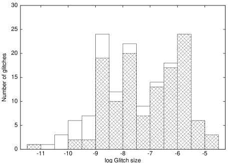
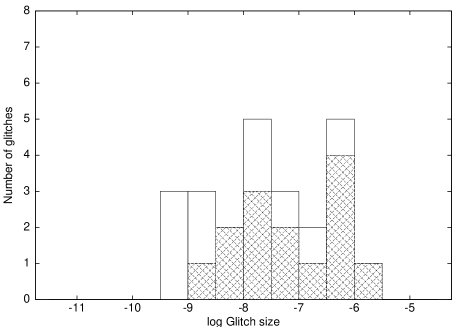
Figure 6: Upper panel: histogram of all known glitch sizes, from the ATNF glitch table  (Manchester et al. 2005) and Urama & Okeke (1999). New glitches found in this study are added on top of the known glitches. The lower panel shows the glitches of PSR B1737$-$30.

4.2 Glitch activity

An indication of glitch activity was first introduced by McKenna & Lyne (1990) as the mean fractional change in the rotation frequency per year due to glitches:

$$A_{g}=\frac{1}{t_{g}}\sum\frac{\Delta\nu}{\nu},$$ (1)

where $\Sigma\frac{\Delta\nu}{\nu}$ is the sum of all glitches occurring in the observed time span $t_{g}$, which is measured in years. They found that the glitch activity is highest for pulsars with low characteric ages and high frequency derivatives. Most young pulsars ($\tau_{c}\lesssim 2000$ yr) show no glitch activity, which is believed to be an effect of higher temperatures reducing the effect of vortex pinning. Apparently for older pulsars, the glitch activity is higher for pulsars with higher spindown rates (e.g. Wang et al. (2000) and Urama & Okeke (1999)).

Our values for glitch activity for pulsars B0740$-$28 and B1737$-$30 are the same as given by Urama & Okeke (1999), see Table 2. However, due to the four mini-glitches in PSR B0355$+$54 and no large glitches in our data span, we calculate a much lower value for the glitch activity of this pulsar than the previously published value including the large glitch seen in this pulsar. Although we find quite a large number of small glitches in the older pulsars of our sample, the derived glitch activity is still low.

4.3 Glitch vs timing noise

Apart from glitches, irregularities in the rotation of the pulsar are usually described as timing noise. Like glitches, timing noise is also seen mostly in the younger pulsars with high spin frequency derivatives. Timing noise is seen as random wanderings in the rotation rate and the timescales range from months to years. Relaxations after glitches are also supposed to be on those timescales. As we are now able to measure smaller and smaller glitches, although not yet including relaxations, it is important to investigate whether small glitches can mimic timing noise.

Arzoumanian et al. (1994) use the parameter $\Delta_{8}$ to quantify the amount of timing noise in a pulsar. They define the parameter as

$$\Delta(t)=\log\left(\frac{1}{6\nu}|\ddot{\nu}|t^{3}\right),$$ (2)

which is usually quoted as $\Delta_{8}$ using a standard time interval of $10^{8}$ seconds. They note that values of $\Delta_{8}$ are expected to vary for non-overlapping data sets. Therefore it is difficult to make a statement about the influence of small glitches on this parameter. What we can do, is compare the value of this parameter for our own data sets, using solutions with glitches and without glitches. If the parameter stays the same, we can conclude that it is not influenced by glitches and the glitches are a different phenomenon than timing noise. Unfortunately, the variation in $\Delta_{8}$ is so large, even for adjacent or partially overlapping intervals of $10^{8}$ seconds in our data, that it is impossible to draw a conclusion from the values.

To make a better distinction, if possible, between timing noise and glitches, more modelling is needed, both on the expected glitch size distributions, as well as on the exact influence on timing parameters of small glitches and recoveries from large glitches. We have seen that for frequently glitching pulsars, it can be difficult to resolve glitches that occur close together in time. This effect is probably more important for small glitches, as they appear to occur more often and thus are more likely to merge together. There are many manifestations of timing noise and some have a form which clearly cannot be explained as being due to glitches. However our discovery of small glitches and the way in which we were able to improve a ”timing-noise-like” set of residuals for PSR B1951$+$32 by including glitches in the solution indicates that they may play a role, and that improved sensitivity and more frequent observations may be required to find more such instances.

Table 3: Glitch parameters for the 30 new glitches found in this study. Where no error in the glitch epoch is quoted, it was not possible to constrain the epoch by using the extra glitch parameter GLPH. In these cases the middle of the interval between adjacent datapoints is quoted as the glitch epoch.

Pulsar name	Epoch (MJD)	$\Delta\nu/\nu(10^{-9})$	$\Delta\dot{\nu}/\dot{\nu}(10^{-3})$
B0355$+$54	51673(15)	000.04(2)
	51965(14)	000.030(2)	00$-$0.102(7)
	52941(9)	000.04(1)	$-$000.13(4)
	53216(11)	000.10(2)	00$-$0.03(4)
B0525$+$21	52289(11)	001.46(5)	$-$000.6(1)
	53379	000.17(5)
B0740$-$28	51770(20)	001.0(3)	$-$000.9(2)
	52027(5)	002.1(2)	00$-$1.1(2)
	53090.2(2.6)	002.9(1)	$-$000.39(3)
	53469.7(8.1)	001.1(2)
B1737$-$30	51685(21)	000.7(4)	$-$000.09(7)
	51822(7)	000.8(3)	00$-$0.07(7)
	52007(6)	000.7(1)	00$-$0.08(2)
	52235	42.1(9)
	52271	444(5)
	52344	220.6(9)
	52603(5)	001.5(1)	00$-$0.60(3)
	52759(5)	001.6(3)	00$-$0.59(8)
	52859	17.6(3)	$-$000.9(1)
	52943.5	22.1(4)
J1814$-$1744	51700(16)	005(2)
	52117(6)	33(2)	00$-$0.5(4)
	53302(22)	007(2)	00$-$2(1)
B1951$+$32	51967(9)	002.25(9)	00$-$0.2(1)
	52385(11)	000.72(9)	00$-$0.04(8)
	52912(5)	001.29(7)	00$-$0.30(9)
	53305(6)	000.51(9)	00$-$0.11(7)
B2224$+$65	51900	000.14(3)	00$-$2.9(2)
	52950	000.08(4)	00$-$1.4(2)
	53434(13)	000.19(6)

Table 4: Glitches in AXPs and high-B radio pulsars. The differences in $\Delta\dot{\nu}/\dot{\nu}$ for the second glitch in 1RXS J1708$-$4009 are due to a different time scale fitted in the papers. Dall’Osso et al. (2003) fit short term change, Kaspi & Gavriil (2003) long-term. See Fig.1b of Kaspi & Gavriil (2003).
References: 1. Dall’Osso et al. (2003), 2. Kaspi & Gavriil (2003) 3.Kaspi et al. (2003), 4. Camilo et al. (2000), 5. this paper.

AXP name	Epoch (MJD)	$\Delta\nu/\nu\leavevmode\nobreak\ (10^{-9})$	$\Delta\dot{\nu}/\dot{\nu}\leavevmode\nobreak\ (10^{-3})$	ref.
1RXS	51459.0	643(5)	$-$0017.2(5)	1
J1708$-$4009	51444.601	549(20)	$-$0010.0(4)	2
	52015.65	330(20)	330(30)a	1
	52014.177	141(27)	$-$0000.1(4)a	2
1E 2259$+$586	52443.9	4100(30)	1110(70)	3
Pulsar name	Epoch (MJD)	$\Delta\nu/\nu\leavevmode\nobreak\ (10^{-9})$	$\Delta\dot{\nu}/\dot{\nu}\leavevmode\nobreak\ (10^{-3})$	ref.
J1119$-$6127	51398	0004.4(4)	$-$0000.039(5)	4
J1814$-$1744	51700	0005(2)		5
	52117	0033(2)	000$-$0.5(4)	5
	53302	0007(2)	$-$0002(1)	5

References

- Arzoumanian et al. (1994) Arzoumanian, Z., Nice, D. J., Taylor, J. H., & Thorsett, S. E. 1994, ApJ, 422, 671
- Backus et al. (1982) Backus, P. R., Taylor, J. H., & Damashek, M. 1982, ApJ, 255, L63
- Camilo et al. (2000) Camilo, F., Kaspi, V. M., Lyne, A. G., et al. 2000, ApJ, 541, 367
- Chatterjee & Cordes (2004) Chatterjee, S. & Cordes, J. M. 2004, ApJ, 600, L51
- Cognard & Backer (2004) Cognard, I. & Backer, D. C. 2004, ApJ, 612, L125
- Cordes & Helfand (1980) Cordes, J. M. & Helfand, D. J. 1980, ApJ, 239, 640
- D’Alessandro et al. (1993) D’Alessandro, F., McCulloch, P. M., King, E. A., Hamilton, P. A., & McConnell, D. 1993, MNRAS, 261, 883
- Dall’Osso et al. (2003) Dall’Osso, S., Israel, G. L., Stella, L., Possenti, A., & Perozzi, E. 2003, ApJ, 599, 485
- Downs (1982) Downs, G. S. 1982, ApJ, 257, L67
- Foster et al. (1990) Foster, R. S., Backer, D. C., & Wolszczan, A. 1990, ApJ, 356, 243
- Foster et al. (1994) Foster, R. S., Lyne, A. G., Shemar, S. L., & Backer, D. C. 1994, AJ, 108, 175
- Gonzalez et al. (2004) Gonzalez, M. E., Kaspi, V. M., Lyne, A. G., & Pivovaroff, M. J. 2004, ApJ, 610, L37
- Hobbs (2002) Hobbs, G. 2002, PhD thesis, University of Manchester
- Hobbs et al. (2005) Hobbs, G., Lorimer, D. R., Lyne, A. G., & Kramer, M. 2005, MNRAS, 360, 974
- Hobbs et al. (2004) Hobbs, G., Lyne, A. G., Kramer, M., Martin, C. E., & Jordan, C. 2004, MNRAS, 353, 1311
- Kaspi & Gavriil (2003) Kaspi, V. M. & Gavriil, F. P. 2003, ApJ, 596, L71
- Kaspi et al. (2003) Kaspi, V. M., Gavriil, F. P., Woods, P. M., et al. 2003, ApJ, 588, L93
- Kaspi & McLaughlin (2005) Kaspi, V. M. & McLaughlin, M. A. 2005, apj, 618, L41
- Krawczyk et al. (2003) Krawczyk, A., Lyne, A. G., Gil, J. A., & Joshi, B. C. 2003, MNRAS, 340, 1087
- Kulkarni et al. (1988) Kulkarni, S. R., Clifton, T. R., Backer, D. C., et al. 1988, Nature, 331, 50
- Lyne (1987) Lyne, A. G. 1987, Nature, 326, 569
- Lyne et al. (2000) Lyne, A. G., Shemar, S. L., & Graham-Smith, F. 2000, MNRAS, 315, 534
- Manchester et al. (2005) Manchester, R. N., Hobbs, G. B., Teoh, A., & Hobbs, M. 2005, AJ, 129, 1993
- Manchester et al. (1972) Manchester, R. N., Taylor, J. H., & Huguenin, G. R. 1972, Nature Phys. Sci., 240, 74
- McKenna & Lyne (1990) McKenna, J. & Lyne, A. G. 1990, Nature, 343, 349
- McLaughlin et al. (2003) McLaughlin, M. A., Stairs, I. H., Kaspi, V. M., et al. 2003, ApJ, 591, L135
- Pivovaroff et al. (2000) Pivovaroff, M., Kaspi, V. M., & Camilo, F. 2000, ApJ, 535, 379
- Ruderman et al. (1998) Ruderman, M., Zhu, T., & Chen, K. 1998, ApJ, 492, 267
- Shabanova (1990) Shabanova, T. V. 1990, Sov. Astron., 34, 372
- Shemar & Lyne (1996) Shemar, S. L. & Lyne, A. G. 1996, MNRAS, 282, 677
- Standish (1982) Standish, E. M. 1982, A&A, 114, 297
- Strom (1987) Strom, R. G. 1987, ApJ, 319, L103
- Urama & Okeke (1999) Urama, J. O. & Okeke, P. N. 1999, MNRAS, 310, 313
- Voûte et al. (2002) Voûte, J. L. L., Kouwenhoven, M. L. A., van Haren, P. C., et al. 2002, A&A, 385, 733
- Wang et al. (2000) Wang, N., Manchester, R. N., Pace, R., et al. 2000, MNRAS, 317, 843
- Wang et al. (2001) Wang, N., Manchester, R. N., Zhang, J., et al. 2001, MNRAS, 328, 855