Searching dark-matter halos in the GaBoDS survey

Abstract

Context. We apply the linear filter for the weak-lensing signal of dark-matter halos developed in Maturi et al. (2005) to the cosmic-shear data extracted from the Garching-Bonn-Deep-Survey (GaBoDS).

Aims. We wish to search for dark-matter halos through weak-lensing signatures which are significantly above the random and systematic noise level caused by intervening large-scale structures.

Methods. We employ a linear matched filter which maximises the signal-to-noise ratio by minimising the number of spurious detections caused by the superposition of large-scale structures (LSS). This is achieved by suppressing those spatial frequencies dominated by the LSS contamination.

Results. We confirm the improved stability and reliability of the detections achieved with our new filter compared to the commonly-used aperture mass (Schneider, 1996; Schneider et al., 1998) and to the aperture mass based on the shear profile expected for NFW haloes (see e.g. Schirmer et al., 2004; Hennawi & Spergel, 2005). Schirmer et al. (2006) achieved results comparable to our filter, but probably only because of the low average redshift of the background sources in GaBoDS, which keeps the LSS contamination low. For deeper data, the difference will be more important, as shown by Maturi et al. (2005).

Conclusions. We detect fourteen halos on about eighteen square degrees selected from the survey. Five are known clusters, two are associated with over-densities of galaxies visible in the GaBoDS image, and seven have no known optical or X-ray counterparts.

1 Introduction

Claims have been made in the literature that dark mass concentrations were significantly detected through their weak-lensing signal (see e.g. Erben et al., 2000; Umetsu & Futamase, 2000; Miralles et al., 2002; Erben et al., 2003). If confirmed, these detections were extremely exciting because they showed that large, dark mass concentrations could exist which for some reason failed to emit light, either as stellar light from galaxies or X-ray emission from hot intracluster plasma. Since the baryon fraction in clusters should faithfully reflect the cosmic mixture of baryonic and dark mass (Ettori et al., 2003, 2006), detections of truly dark cluster-sized halos could shed doubt on our understanding of the formation of non-linear cosmic structures.

Obviously, gravitational lensing is the only method able to detect dark mass concentrations. This strength is also its weakness: all density inhomogeneities projected along the line-of-sight cause gravitational light deflection, thus any detection of a lensing signal possibly due to a dark-matter halo is affected to some degree by the large-scale structures projected into the observed field. Superpositions of large-scale structures can create signals mimicking dark-matter halos.

Commonly used methods for detecting halos through weak lensing, in particular the aperture mass (Schneider, 1996; Schneider et al., 1998), are optimised for measuring the total projected mass enclosed within an aperture, and for suppressing the cross-correlation of the signal in neighbouring apertures.

A clean separation between the signals of halos and large-scale structures is strictly impossible because the large-scale structure can be considered as composed of halos with a broad mass spectrum. Unambiguous noise suppression can thus not be achieved. However, we have argued in (Maturi et al., 2005) that the weak-lensing power spectrum obtained from the linearly evolved dark-matter power spectrum can reasonably be considered as a noise contribution against which the weak-lensing signal of halos can be filtered. The underlying assumption is that those halos which we are searching for do in fact create the non-linear power spectrum.

Using simulations, we demonstrated that the linear filter which follows uniquely from this noise model and the assumption that dark-matter halos on average have an NFW density profile does indeed perform as expected (Maturi et al., 2005). It suppresses the noise from large-scale structures substantially, thus considerably reducing the number of spurious detections, and is much less sensitive than the aperture mass against changes in the filter scale. Removing the LSS contamination is less important for relatively shallow observations, i.e. for average source redshifts $z_{\mathrm{s}}\lesssim 1$, but it is fundamental for deep observations in which the integrated contribution of the matter along the line-of-sight becomes non-negligible.

We now apply this filter to the weak-lensing data obtained from the Garching-Bonn-Deep-Survey (hereafter GaBoDS, see Schirmer et al., 2003). The purpose of this study is two-fold. First, we wish to compare the halo detections with the new filter and with the aperture mass, and second, we want to assess the reliability of the halo detections and their stability against changes in the filter scale.

We emphasise that we do not want to devaluate the aperture mass. It was shown to have many desirable properties for the measurement of cosmic shear. However, its construction for a different purpose than halo detection motivates us to search for an alternative measure. Ultimately, our filter can be seen as a variant of the aperture mass based on a considerably narrower angular weight function, which is characterised by the assumed halo density profile and the noise model.

Throughout, we assume that dark matter halos have density profiles of NFW shape and use the angular scale radius of the profile as a free parameter. Moreover, we compute the weak-lensing power spectrum of linear large-scale structures adopting a $\Lambda$CDM cosmological model, with $\Omega_{0}=0.3$, $\Omega_{\Lambda}=0.7$, $\sigma_{8}=0.9$ and $h=0.7$.

The paper is structured as follows: Sect. 2 briefly summarises the survey characteristics; Sects. 3 and 4 describe the aperture mass and our optimal filter, respectively; and Sect. 5 presents the analysis of the data sample. Our conclusions are presented in Sect. 6.

2 The GaBoDS survey

The Garching-Bonn Deep Survey collects observations obtained with the Wide Field Imager (WFI) mounted on the MPG/ESO 2.2m telescope. The survey covers $\sim 19$ square degrees in the $R$ band and consists of shallow ($4-7\,\mbox{ksec}$, $9.6\,\mbox{deg}^{2}$), medium ($8-11\,\mbox{ksec}$, $7.4\,\mbox{deg}^{2}$) and deep ($13-56\,\mbox{ksec}$, $2.6\,\mbox{deg}^{2}$) exposures taken under sub-arcsecond seeing conditions. To a large extent, the data constitute a virtual survey in the sense that a very substantial fraction of it was identified in the ESO archive.

The fields are randomly distributed in the southern sky and at high Galactic latitude, avoiding bright stars, extended foreground objects and to some degree also known massive galaxy clusters (for more details see Schirmer et al. 2003).

The number density of galaxies used for our weak lensing study reflects the inhomogeneous depth of the survey and ranges from $n=6-24\,\mbox{arcmin}^{-2}$, with an average of $\bar{n}\approx 12\,\mbox{arcmin}^{-2}$.

A comprehensive characterisation of the survey can be found in (Schirmer et al., 2003), including references to its suitability for weak lensing studies. The data reduction was performed with the THELI pipeline, which Erben et al. (2005) describe in detail.

3 Aperture mass

The aperture mass is widely used for weak-lensing studies. It is defined as a weighted integral of the local convergence,

$$M_{\mathrm{ap}}(\@vec{\theta})=\int\mathrm{d}^{2}\theta^{\prime}\,\kappa(\@vec{\theta}^{\prime})U(\@vec{\theta}-\@vec{\theta}^{\prime})\;,$$ (1)

where the aperture is chosen to be circular and $U$ is a compensated axially symmetric weight function, i.e. it satisfies

$$U(\theta) = U(|\@vec{\theta}|)$$ (2)

$$= \int_{0}^{\theta}\mathrm{d}\theta^{\prime}\,\theta^{\prime}\,U(\theta^{\prime})=0\;.$$ (3)

Figure 1: Comparison between the filter profiles. Different line types refer to the conventional aperture mass (solid line), the optimal filter described in this paper but without the large-scale structure contribution to the noise power spectrum (dashed line), the full optimal filter for $r_{s}=2^{\prime}$ and $r_{s}=4^{\prime}$ (heavy solid and heavy dash-dotted lines, respectively). The large-scale structure power spectrum modifies the filter shape according to the filter scale by lowering its sensitivity on large scales where weak lensing by large-scale structure dominates.

Since the convergence is not directly measurable, Eq. (1) is conveniently expressed in terms of the shear component $\gamma_{\mathrm{t}}$ tangential with respect to the aperture centre $\@vec{\theta}$ on the sky, and can be written in the form

$$M_{\mathrm{ap}}(\@vec{\theta})=\int\mathrm{d}^{2}\theta^{\prime}\,\gamma_{\mathrm{t}}(\@vec{\theta}^{\prime})Q(|\@vec{\theta}-\@vec{\theta}^{\prime}|)\;,$$ (4)

where the function $Q$ is related to $U(\theta)$ through

$$Q(\theta)\equiv\frac{2}{\theta^{2}}\int_{0}^{\theta}\mathrm{d}\theta^{\prime}\,\theta^{\prime}\,U(\theta^{\prime})-U(\theta)\;.$$ (5)

The function $Q$ is usually chosen to have a compact support, which is adequate for the finite data fields on which halos are sought. It is also typically chosen to suppress the halo centre because there the tangential component of the ellipticity is not defined, the weak-lensing approximation may break down, and cluster galaxies may prevent the shapes of background galaxies from being precisely measured.

Schneider et al. (1998) proposed a polynomial shape for $Q$,

$$Q_{\mathrm{pol}}(x)=\frac{(1+l)(2+l)}{\pi\theta^{2}}\,x^{2}(1-x^{2})^{l}\mathrm{H}(1-x)\,,$$ (6)

where $\mathrm{H}$ is the Heaviside step function, $l$ is a free parameter usually set to $l=1$, $x\equiv\theta/\Theta$ and $\Theta$ is the radius where $Q$ vanishes.

These filter profiles do not minimise the variance of the estimate $M_{\mathrm{ap}}$, and their aperture can be arbitrarily chosen by the observer, leading to unstable results which sensitively depend on the filter scale (Maturi et al., 2005). It was designed for cosmic shear statistics, but it is widely used in the literature for halo searches.

In recent years, other function types have been introduced for $Q$ in order to maximise the signal-to-noise ratio. Schneider et al. (1998) showed that this is achieved if $Q$ mimics the tangential shear profile of the lens. For example, Schirmer et al. (2004); Hennawi & Spergel (2005) and Padmanabhan et al. (2003) use functions which approximate the expected shear profile of a NFW halo.

Specifically, Schirmer et al. (2004) used the following parameterisation

$$Q_{\mathrm{tanh}}(x)=\frac{1}{1+\mathrm{e}^{6-150x}+\mathrm{e}^{-47+50x}}\frac{\tanh(x/x_{\mathrm{c}})}{x/x_{\mathrm{c}}}\,,$$ (7)

where $x_{\mathrm{c}}$ defines how peaked the profile is in analogy to the scale radius of the NFW profile. The exponential pre-factor damps the filter within its inner and outermost 10%.

However, all these functions have some disadvantage since they neglect the presence of the cosmic shear from large-scale structures which dominates the halo lensing signal above some scale and thus acts as an intense source of noise.

4 Optimal filter

Table 1: GaBoDS fields rejected because of an excessive $B$-mode contamination. Each column lists the names of the rejected fields, where the selection was performed for each filter and all scales because they determine the sensitivity for the residual $B$-mode.

$M_{ap}$ 4’	$M_{oap}$ 10’	$M_{oap}$ 20’	$A_{opt}$ 2’	$A_{opt}$ 4’
A1347_P3	-	-	-	-
-	-	A1347_P4	-	-
B8m3	-	-	-	-
-	-	B8p0	-	B8p0
B8p2	-	-	-	-
-	-	B8p3	-	B8p3
-	-	C0400	-	C0400
C04p3	C04p3	C04p3	C04p3	C04p3
CL1119	-	-	-	-
-	-	Cl1301	-	-
-	-	-	-	DEEP3b
FDF	-	-	-	-
-	Pal3	Pal3	Pal3	Pal3
SGP	-	-	-	-

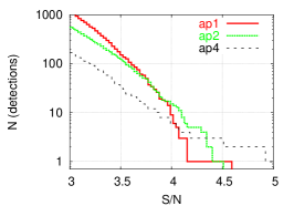
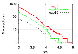
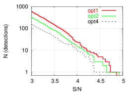
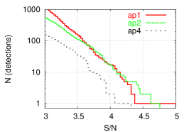
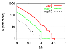
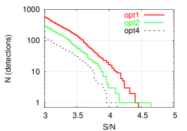
Figure 2: Cumulative distribution of the S-detections (upper panels) and of the N-detections (bottom panels) as a function of their signal-to-noise ratio. Three filter functions were used: the aperture mass $M_{\mathrm{ap}}$ as described by Schneider (1996) (left panels), the aperture mass $M_{\mathrm{oap}}$ as defined by Schirmer et al. (2004) (middle panels), and the optimal filter $A_{\mathrm{opt}}$ developed by Maturi et al. (2005) (right panels). Three different scales were used: $1^{\prime}$, $2^{\prime}$ and $4^{\prime}$ for $M_{\mathrm{ap}}$ and $A_{\mathrm{opt}}$, and $5^{\prime}$, $10^{\prime}$ and $20^{\prime}$ for $M_{\mathrm{oap}}$. The number of spurious N-detections is high with all filters. However, only with $M_{\mathrm{oap}}$ and $A_{\mathrm{opt}}$ have the distributions of S-detections a tail extending towards high signal-to-noise ratio for all filter scales, exceeding the number of noise detections. A comparison between the distributions of the S-detections and of the N-detections is more clearly shown in Fig. (3).

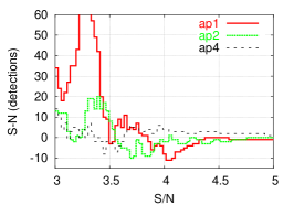
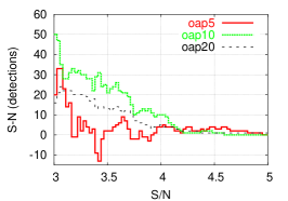
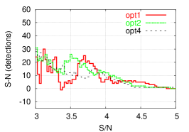
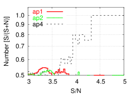
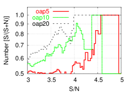
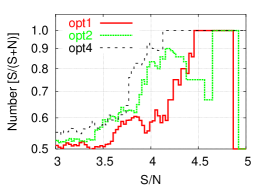
Figure 3: In order to more clearly compare the S- and N-distributions for each filter, we plot their difference (upper panels) and the ratio between the S-distribution and the sum of the S- and N-distributions (bottom panels). The original aperture mass $M_{\mathrm{ap}}$ (left panels) shows a significant contribution of S-detections only for an aperture of $4^{\prime}$. In comparison, $M_{\mathrm{oap}}$ (middle panels) and $A_{\mathrm{opt}}$ (right panels) give a net positive contribution for large signal-to-noise ratios on all scales. Consequently, it is possible to define a threshold S/N ratio above which the detections can be considered reliable. This plot underlines the superior statistical properties of the two optimised filters compared to the aperture mass $M_{\mathrm{ap}}$. It also shows that $A_{\mathrm{opt}}$ yields more reliable and stable results than the other filters. In fact, at high signal-to-noise ratios, it produces the largest difference between S- and N-detections.

As discussed by Maturi et al. (2005), we shall model this weak-lensing contribution as a noise component to be filtered out. The measured data $D(\@vec{\theta})$ is thus composed by the signal $S(\@vec{\theta})$ and some noise $N(\@vec{\theta})$,

$$D(\@vec{\theta})=S(\@vec{\theta})+N(\@vec{\theta})=A\tau(\@vec{\theta})+N(\@vec{\theta})\;,$$ (8)

expressing that the signal is modelled as the weak-lensing signal of a dark-matter halo with amplitude $A$ and angular shape $\tau(\@vec{\theta})$. We assume $\tau$ is axially symmetric on average, thus $\tau(\@vec{\theta})=\tau(|\@vec{\theta}|)$. Since the signal contained in our data $D$ is the reduced shear $g$, we now identify $\tau$ with the reduced shear expected from a given halo model, and approximate the reduced shear by the shear $\gamma$. This is justified for weak-lensing, $\kappa\ll 1$.

The noise component $N$ is assumed to be random with zero mean and isotropic, since to sufficient approximation the background galaxies are randomly placed and oriented, and weak lensing by large-scale structures is well described by an isotropic Gaussian random field. The variances of the noise components are conveniently described in the Fourier domain, where their correlation functions are given by the power spectrum

$$\langle\hat{N}(\@vec{k}^{\prime})^{*}\hat{N}(\@vec{k})\rangle=(2\pi)^{2}\,\delta(\@vec{k}^{\prime}-\@vec{k})P_{N}(k)\;.$$ (9)

The hats above symbols denote their Fourier transforms, and $P_{N}(k)$ is the noise power spectrum. Thus the noise given by the intrinsic ellipticity of the sources combined with their finite number is modelled by its power spectrum $P_{\epsilon}$, and the noise caused by weak lensing of intervening large-scale structures is modelled by the cosmic-shear power spectrum $P_{\gamma}$ derived from the linear dark-matter power spectrum. The complete noise power spectrum is thus

$$P_{N}(k)=P_{\epsilon}(k)+P_{\gamma}(k)=\frac{1}{2}\frac{\sigma_{\epsilon_{\mathrm{s}}}^{2}}{n_{\mathrm{g}}}+\frac{1}{2}\,P_{\gamma}(k)\;,$$ (10)

where the factor $1/2$ arises because only one (the tangential) component of the ellipticity contributes to the measurement. The linear filter $\Psi(\@vec{\theta})$ is constructed to yield an estimate $A_{\mathrm{est}}$ for the amplitude $A$ of the signal at position $\@vec{\theta}$,

$$A_{\mathrm{est}}(\@vec{\theta})=\int D(\@vec{\theta}^{\prime})\Psi(\@vec{\theta}-\@vec{\theta}^{\prime})\,\mathrm{d}^{2}\theta^{\prime}\;,$$ (11)

which is unbiased, i.e. the mean error has to vanish $b\equiv\langle A_{\rm est}-A\rangle=0$, and minimises the measurement noise $\sigma^{2}\equiv\left\langle(A_{\mathrm{est}}-A)^{2}\right\rangle$. A filter $\Psi$ satisfying these two conditions is found by introducing a Lagrangian multiplier $\lambda$ and searching for the function $\Psi$ which minimises the functional $L[\Psi]=\sigma^{2}+\lambda b$. This yields

$$\hat{\Psi}(\@vec{k})=\frac{1}{(2\pi)^{2}}\left[\int\frac{|\hat{\tau}(\@vec{k})|^{2}}{P_{N}(k)}\mathrm{d}^{2}k\right]^{-1}\,\frac{\hat{\tau}(\@vec{k})}{P_{N}(k)}\;.$$ (12)

By construction, the filter $\Psi$ is thus most sensitive for those spatial frequencies where the signal $\hat{\tau}$ is large and the noise $P_{N}(k)$ is low (for details see Maturi et al., 2005).

Throughout the paper, we assume that the signal is faithfully modelled by the shear of an NFW profile (see e.g. Bartelmann, 1996; Wright & Brainerd, 2000; Li & Ostriker, 2002; Meneghetti et al., 2003). Consequently, the filter is optimised to detect the same halo shape as the optimised aperture mass given by Eq. (7). We emphasise that, in contrast to the aperture mass, this filter is not constructed from an arbitrary compensated filter function for the convergence, but defined such that it maximises the signal-to-noise ratio and minimises the contamination induced by the LSS or, in principle, by any Gaussian noise with known power spectrum. It has the further advantage of being more stable against changes of the filter size, due to the shape control imposed by the noise power spectrum. Thus, like the aperture mass, this approach is based on an ordinary convolution (11) of the data with a filter $\Psi$ or $Q$, but its signal-to-noise properties differ from that of the aperture mass because they are determined by the specific choice of the filter. The different filter profiles are compared in Fig. (1).

To fully exploit these properties, deep observations with a high galaxy number density are needed, because if the shot noise is dominant with respect to the LSS noise, its performance is expected to be comparable to the optimised aperture mass.

5 Analysis of the GaBoDS data

The GaBoDS survey data are fully analysed by Schirmer et al. (2006) (hereafter [S06]), who aim at compiling a list of candidate dark-matter halos which is as complete as possible. They are selected with the aperture mass $M_{\mathrm{ap}}$ combined with a different statistic evaluating the probability for finding a cluster with a given S/N at a particular position. The latter is also based on $M_{\mathrm{ap}}$ ; see [S06] for details. They find 158 detections, $\sim 50\%$ of which coincide with galaxy over-densities visible in the GaBoDS images.

In the present analysis based on the filter $\Psi$ optimised for suppressing the noise, we reject all detections below a minimum signal-to-noise ratio. This threshold is motivated by a statistical analysis performed on the same data (see Sect. 5.3), even if they coincide with known clusters or galaxy overdensities. In this way, we obtain a list which is shorter than that obtained by [S06], but contains only those detections which are statistically reliable.

We also present a statistical comparison between the results obtained with our optimal filter and with the two versions of the aperture mass.

5.1 Formalism for discrete data

Since our estimation is performed on discrete sources, the integral in Eqs. (4) and (11) must be approximated by a sum over the background galaxies,

$$A_{\mathrm{est}}(\@vec{\theta})=\frac{1}{n_{\mathrm{g}}}\,\sum_{i}\epsilon_{\mathrm{t}i}(\@vec{\theta}_{i})\,\Psi(|\@vec{\theta}_{i}-\@vec{\theta}|)\;.$$ (13)

The noise estimate in $A_{\mathrm{est}}$ is obtained from the variance definition $\sigma^{2}\equiv\left\langle(A_{\mathrm{est}}-A)^{2}\right\rangle$ as

$$\sigma^{2}_{A_{\mathrm{est}}}(\@vec{\theta})=\frac{1}{2n_{\mathrm{g}}^{2}}\,\sum_{i}|\epsilon_{\mathrm{t}i}(\@vec{\theta}_{i})|^{2}\Psi^{2}(|\@vec{\theta}_{i}-\@vec{\theta}|)\;,$$ (14)

where $n_{\mathrm{g}}$ is the number density of sources, $\epsilon_{\mathrm{t}i}(\@vec{\theta}_{i})$ denotes the tangential component of the $i$th galaxy’s ellipticity relative to the line connecting $\@vec{\theta}_{i}$ and $\@vec{\theta}$. Thus, the filtering is performed in the real domain, which requires to Fourier back-transform the filter function from Eq. (12). Equation (14) is a good approximation where the local shear is negligible compared to the intrinsic galaxy ellipticities, but it will typically fail near clusters. This limitation can be overcome by substituting the variance of the intrinsic galaxy ellipticities measured in the entire field.

Since the aperture mass and the optimal filter use the same linear estimator, this discretisation is also used for the aperture mass, by substituting $Q$ for $\Psi$ in Eqs. (13) and (14).

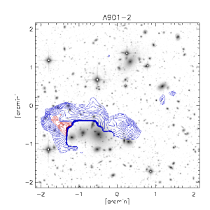
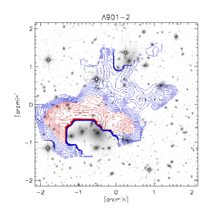
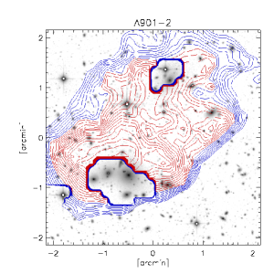
Figure 4: Example of a weak-lensing detection obtained with the optimal filter $A_{\mathrm{opt}}$ for the three different filter scales adopted in this study; $1^{\prime}$, $2^{\prime}$ and $4^{\prime}$. The signal-to-noise iso-contours of the weak-lensing signal are superimposed here on the R-band image. The panel has a side length of $4.3^{\prime}$, and the iso-contour lines start from $S/N=3$ with a step width of $0.1$. The red iso-contours are for $S/N>4.37$, $S/N>4.12$ and $S/N>3.90$, respectively, and mark the reliable detections for each filter scale. Note the mask applied to remove bright galaxies and stars from the weak-lensing data.

5.2 Signal-to-noise maps

Using Eqs. (13) and (14), we produce maps of the signal-to-noise ratio for all our fields, henceforth called S-maps, using the aperture masses $M_{\mathrm{ap}}$ and $M_{\mathrm{oap}}$ given by Eqs. (6) and (7), and the optimal filter $A_{\mathrm{opt}}$ given by Eq. (12). The optimal filter $\Psi$ used in $A_{\mathrm{opt}}$ is computed for each field, because it has to be optimised according to the observed galaxy number density. We use different filter sizes to test the stability of the results achieved.

In order to investigate the noise properties of our data and to test the reliability of the detections, we repeated the analysis on data catalogues in which all individual shear measurements were rotated with a phase angle of $45$ degrees, deleting any lensing signal contained in the data. The analysis of these “rotated” data sets yields signal-to-noise maps similar to the previous S-maps, but containing only noise due to the residual $B$-modes and to the shot noise present in the data, and where no detections caused by lensing can be found. We call these maps N-maps.

We define the detections from the S- and N-maps as peaks above a given S/N threshold and call them S- and N-detections, respectively. The detections are automatically identified using a friends-of-friends (FF) algorithm which finds groups of pixels on the S- and the N-maps connected with a linking length of $1^{\prime}$. This procedure avoids that S/N peaks associated with the same distortion pattern are identified as different detections. In fact, the signal given by a single halo can be fragmented by the noise, especially for low signal-to-noise ratios and small filter scales, for which the shot noise is more relevant.

We reject all fields where the noise given by the residual $B$-mode, as detected in the N-maps, gives spurious detections which are not compatible with the typical properties of the noise of our full data sample, i.e. with signal-to-noise ratios and angular extentions belonging to extended tails in the respective distributions. This selection has only a small impact on the final detection sample. The selection of these fields depends on the filter used, because of their different sensitivity on different scales. Our analysis revealed that this contamination is larger for filters with a larger aperture, as can be seen in Tab. (1), where we list the rejected fields.

In Sect. (5.3) we discuss the statistical properties of the detections, defining a threshold criterion which justifies the reliability of the peaks described in Sect. (5.4).

5.3 Statistics of the detections

The statistical properties of the S- and N-detections, described in Sect. (5.2), are shown in the upper and lower panels of Fig. (2), respectively. There, we plot the cumulative distributions of the number of detections as a function of their maximum signal-to-noise ratio. The curves are shown for $M_{\mathrm{ap}}$ (left panels), $M_{\mathrm{oap}}$ (middle panels) and $A_{\mathrm{opt}}$ (right panels). Each filter was used with three different scales; $1^{\prime}$, $2^{\prime}$ and $4^{\prime}$ for $M_{\mathrm{ap}}$ and $A_{\mathrm{opt}}$, and $5^{\prime}$, $10^{\prime}$ and $20^{\prime}$ for $M_{\mathrm{oap}}$.

All filters find many spurious N-detections, but the statistical properties of data allow us to define a criterion to identify only the most reliable detections. In fact, for $M_{\mathrm{oap}}$ and $A_{\mathrm{opt}}$ only, the N-distribution drops faster than the S-distribution, and for signal-to-noise ratios larger than a threshold depending on the filter, no spurious detections are found. This defines the signal-to-noise threshold to be used in selecting the detections.

To better compare the S- and N-distributions for each filter, we plot in Fig. (3) their difference (upper panels) and the ratio between the S- and the sum of the S- and the N-distributions (bottom panels). The bottom panels show only the range between $0.5$ and $1$, i.e. where the number of S-detections is at least as high as the number of N-detections. The figure clearly shows that the number of N-detections at high signal-to-noise ratios obtained with $M_{\mathrm{ap}}$ (left panels) is comparable or even larger than the number of S-detections except for an aperture of $4^{\prime}$. Consequently, this filter does not allow any distinction between real detections and noise peaks, showing a strong dependence on the chosen aperture. In comparison, the detections with $M_{\mathrm{oap}}$ and $A_{\mathrm{opt}}$, shown in the centre and right panels respectively, have substantially improved properties. Their S-detection distributions have a tail extending towards high signal-to-noise ratios, rising above the number of noise detections. As mentioned before, this shows that it is possible with these filters to define a signal-to-noise threshold where the number of N-detections drops below the number of S-detections. Detections above this threshold define reliable peaks for all scales.

Applied to the GaBoDS data analysed here, even though $M_{\mathrm{oap}}$ performed less well than $A_{\mathrm{opt}}$, it returned almost comparable results. This is not surprising because the filter shapes are based on the same model for the halo density profiles. Thus, the only decisive difference is that $A_{\mathrm{opt}}$ additionally suppresses the noise contribution of the LSS. The low number density of galaxies in the GaBoDS survey and their low average redshift tend to reduce this difference. However, this additional feature should be of primary importance in deeper surveys such as the Cosmic Evolution Survey, whose average source redshift is higher, increasing the amount of matter projected along the line-of-sight and consequently the contamination it causes.

5.4 The significant weak-lensing detections

Since $A_{\mathrm{opt}}$ and $M_{\mathrm{oapt}}$ return similar results, but the former has the further advantage of yielding the most reliable and stable detections, we analyse only its results in detail.

Given the noise properties of our data sample and if we consider $\sim 2$ spurious detections on the whole sample of about 18 square degrees an acceptable contamination, the lower signal-to-noise threshold described in Sect. (5.3) is fixed at $4.37$, $4.12$ and $3.90$ for the three adopted filter scales of $1^{\prime}$, $2^{\prime}$ and $4^{\prime}$ respectively.

Table 2: List of all reliable detections obtained with the optimal filter with scales of $1^{\prime}$, $2^{\prime}$ and $4^{\prime}$. The adopted signal-to-noise thresholds are $4.37$, $4.12$ and $3.90$ according the filter scale. The columns give a preliminary name for the detections, their coordinates (2000.0), the signal-to-noise ratios obtained with the three filter scales, the number of galaxies per square arc minute in the respective field, the class of the detection (see the text for further explanation, Sect. 5.4), the name of a corresponding object if present, and its redshift. The objects labeled [S06] are the detections obtained with the aperture mass by Schirmer et al. (2006). The signal-to-noise ratios in brackets are below the signal-to-noise threshold.

ID	$\alpha$ (2000.0)	$\delta$ (2000.0)	opt $1^{\prime}$	opt $2^{\prime}$	opt $4^{\prime}$	n	class	object	z
			$4.37<S/N$	$4.12<S/N$	$3.90<S/N$
A901-1	09 56 30	-09 57 10	4.60	4.91	5.22	25	1	A901a	0.16
A901-2	09 55 38	-10 09 46	4.43	4.21	(3.61)	25	3	J095538.2-101019	0.169
AM1-1	03 53 26	-49 42 49	4.86	4.63	4.05	11	6	023 [S06]	–
B8p2-1	22 40 33	-08 23 23	(3.99)	4.19	4.36	11	5	089 [S06]	–
C04p2-1	14 18 58	-11 25 19	(4.34)	4.13	(3.47)	8	4	098 [S06]	–
CL1037-1243-1	10 38 24	-12 32 38	(3.95)	(3.97)	3.97	8	4	–	–
CL1119-1129-1	11 18 22	-11 27 12	(4.26)	4.33	4.01	9	4	058 [S06]	–
Deep1a-1	22 54 02	-40 07 13	4.40	4.34	4.12	14	4	ESP 38	0.151
Deep1b-1	22 50 25	-40 05 55	(3.85)	(4.07)	4.15	8	5	–	–
Deep3d-1	11 18 45	-21 35 57	4.68	4.55	4.27	15	6	060 [S06]	–
Deep3d-2	11 17 37	-21 34 16	4.55	4.34	3.96	15	4	057 [S06]	–
F17_P1-1	14 26 38	-34 46 08	(4.13)	4.25	4.12	7	5	–	–
S11-1	11 43 34	-01 45 42	(3.91)	4.15	4.32	18	1	A1364	0.107
SGP-1	00 45 21	-29 23 31	(3.89)	(3.92)	3.97	25	1	LIL004521-292335	0.257

According to this selection criterion, we identify the candidate dark-matter halos from the data sample, keeping the contamination by spurious detections under control by definition of the filter. Doing so, we obtain a reliable sample consisting of $6$, $11$ and $12$ detections for the three apertures, respectively. These detections are not independent, i.e. most of them are achieved with more than one aperture size, confirming the stability of our filter. Thus, our selected sample of $14$ detections is composed as follows:

• 5 previously known clusters;

• 4 of class 4;

• 5 of class 5-6.

Five of our detections correspond to known clusters listed in the SIMBAD Astronomical Database: Abell 1364, Abell 901, J095538.2$-$101019, ESP 38 and LIL004521$-$292335. The classification of the other detections is given according to the galaxy concentration observed in the images according to the following empirical classes: (1) very clear over-density with more than 50 bright galaxies; (2) clear over-density of 35-50 bright galaxies; (3) still highly significant over-density of 25-35 galaxies; (4) still significant over-density of 15-25 galaxies; (5) very loose distribution of 5-15 galaxies; (6) absence of any kind of galaxy over-density. We use these categories to facilitate the comparison of our detections with the GaBoDS images. We are aware that this scheme may be questionable for the classification of galaxy clusters.

Table (2) lists all candidates with their characteristics. The columns, from left to right, give a preliminary name for the detections, their coordinates (2000.0), the signal-to-noise ratios achieved with the three adopted filter scales, the number of galaxies per square arc minute of the respective fields, the classification of the detection, the name of the corresponding object (if known) and its redshift. The objects labeled [S06] are the detections obtained by Schirmer et al. (2006) by using different combinations of the aperture-mass. The signal-to-noise ratios in brackets are lower than the thresholds of statistically reliable detections.

Recall that we rejected all detections below the thresholds even if associated with known clusters. This is so for LIL004608.1$-$292340 and LIL004544.0$-$294757, which are detected at $3.76\sigma$ and $3.83\sigma$, respectively. This is because we want to carry out a blind search for candidate clusters based exclusively on weak lensing data.

An example for a detection is shown in Fig. (4) where we plot the optical R-band image of the cluster Abell 901 with iso-contours of the signal-to-noise ratio of the weak-lensing signal superimposed. The three panels, with a side length of $4.3^{\prime}$ each, are obtained with the three filter scales adopted in this work. The iso-contour lines start from $S/N=3$ with a step width of $0.1$. The levels of the red iso-contours are at $S/N>4.37$, $S/N>4.12$ and $S/N>3.90$, respectively, and mark the reliable detections for each filter scale. To be conservative, we avoid to compute the signal-to-noise ratio where the bright galaxies and stars were masked from the data. The cluster Abell 901 is a massive structure at redshift $z=0.16$. Due to its size, a filter optimised for larger scales yields higher signal-to-noise ratios, and the extent of the dark matter halo is better visible (see the right panel).

6 Conclusions

The application of our filter to the GaBoDS weak-lensing survey confirms the expectations on its performance raised by Maturi et al. (2005) based on numerical simulations. Our filter is more stable than the aperture mass against changes of the filter size, thus considerably simplifying the interpretation of data. It has better statistical properties compared to the aperture mass given by Eq. (6), yielding more reliable results. Although our filter and the optimised aperture mass given by Eq. (7) perform comparably on the GaBoDS data, the LSS suppression characterising our filter will be primarily important for deeper observations, for which the average background-galaxy redshift will be larger than in GaBoDS and the LSS will not be negligible.

We measured in our data sample a large contamination from residual $B$-modes, but a statistical analysis of the noise properties allowed us to define a criterion to select a sample of reliable detections. We emphasise that a data reduction procedure which minimises the residual $B$-mode is of fundamental importance for the detection of new cluster-sized dark-matter halos.

We rejected all detections below the thresholds even if associated with know clusters, because we wish to search blindly for candidate clusters based exclusively on weak-lensing data. On the $19.6$ square degrees covered by the GaBoDS data, we found $14$ detections with a sufficiently high signal-to-noise ratio, $5$ of which are known clusters, 4 are associated with concentrations of galaxies visible in our data, and 5 detections are not associated with any visible concentration of galaxies. Deep optical and $X$-ray follow-ups of the $9$ unknown detections should be performed to clarify their nature.