Crushing of interstellar gas clouds in supernova remnants

Abstract

Context. X-ray observations of evolved supernova remnants (e.g. the Cygnus loop and the Vela SNRs) reveal emission originating from the interaction of shock waves with small interstellar gas clouds.

Aims. We study and discuss the time-dependent X-ray emission predicted by hydrodynamic modeling of the interaction of a SNR shock wave with an interstellar gas cloud. The scope includes: 1) to study the correspondence between modeled and X-ray emitting structures, 2) to explore two different physical regimes in which either thermal conduction or radiative cooling plays a dominant role, and 3) to investigate the effects of the physical processes at work on the emission of the shocked cloud in the two different regimes.

Methods. We use a detailed hydrodynamic model, including thermal conduction and radiation, and explore two cases characterized by different Mach numbers of the primary shock: ${\cal M}=30$ (post-shock temperature $T_{\rm psh}\approx 1.7$ MK) in which the cloud dynamics is dominated by radiative cooling and ${\cal M}=50$ ($T_{\rm psh}\approx 4.7$ MK) dominated by thermal conduction. From the simulations, we synthesize the expected X-ray emission, using available spectral codes.

Results. The morphology of the X-ray emitting structures is significantly different from that of the flow structures originating from the shock-cloud interaction. The hydrodynamic instabilities are never clearly visible in the X-ray band. Shocked clouds are preferentially visible during the early phases of their evolution. Thermal conduction and radiative cooling lead to two different phases of the shocked cloud: a cold cooling dominated core emitting at low energies and a hot thermally conducting corona emitting in the X-ray band. The thermal conduction makes the X-ray image of the cloud smaller, more diffuse, and shorter-lived than that observed when thermal conduction is neglected.

1 Introduction

This paper is part of a series devoted to study the interaction of a shock wave of an evolved supernova remnant (SNR) with a small interstellar gas cloud (like the ones observed, for instance, in the Cygnus loop or in the Vela SNR) through detailed and extensive numerical modeling. The project aims at overcoming some of the limitations found in the previous analogous studies (for instance, taking into account simultaneously important physical effects such as heat flux and radiative losses) and crucial for the accurate interpretation of the high resolution multi-wavelength observations of middle-aged SNR shell available with the last-generation observatories.

In a previous paper (Orlando et al. 2005; hereafter Paper I), we have modeled in detail the shock-cloud interaction with hydrodynamic simulations including the effects of thermal conduction and radiative losses from an optically thin plasma. We have investigated the interplay of the latter two processes on the cloud evolution and on the mass and energy exchange between the cloud and the surrounding medium, by exploring two different physical regimes in which one of the two processes is dominant. We have found that, when the radiative losses are dominant, the shocked cloud fragments into cold, dense, and compact filaments surrounded by a hot corona gradually ablated by the thermal conduction; to the contrary, when the thermal conduction is dominant, the shocked cloud evaporates in a few dynamical time-scales. In both cases we have found that the thermal conduction is very effective in suppressing the hydrodynamic instabilities that would develop at the cloud boundaries.

In this paper, we study and discuss the time-dependent X-ray emission predicted by the modeling mentioned above. Several authors have investigated the emission from SNRs in different spectral bands, adopting global SNR models including the effects of radiative cooling, evaporating clouds, large scale gradients for the ISM density etc. (e.g Cowie et al. 1981, White & Long 1991, Cox et al. 1999, Shelton et al. 1999, Hnatyk & Petruk 1999, Petruk 2001, Velázquez et al. 2004). On the other hand, the X-ray emission originating from model shocked interstellar clouds has not been investigated yet in detail, despite it is potentially important for the energy budget of the shocked ISM and for the interpretation of the observations.

Here we synthesize from the numerical simulations described in Paper I the X-ray emission expected from the shock-cloud interaction. Our scope includes: 1) to link modeled to X-ray emitting structures, 2) to investigate the emission of the shocked cloud in two different physical regimes in which either thermal conduction or radiative cooling is dominant, and 3) to investigate the effects of thermal conduction and radiation on the emission of the shocked cloud.

The paper is structured as follows: in Sect. 2 we briefly summarize the model of the shock-cloud collision and outline the method to synthesize the X-ray emission from the numerical simulations; in Sect. 3 we discuss the results; and finally in Sect. 4 we draw our conclusions.

2 The modeling

2.1 Hydrodynamic simulations

In this section, we summarize the model of the shock-cloud collision. We refer the reader to Paper I for more details.

The model describes the impact of a planar shock front onto an isolated gas cloud. The cloud before the impact is assumed to be spherical with radius $r_{\rm cl}=1$ pc, small compared to the curvature radius of the SNR shock, internally isothermal, and in pressure equilibrium with the surrounding medium. The unperturbed ambient medium is assumed to be isothermal (with temperature $T_{\rm ism}=10^{4}$ K, corresponding to an isothermal sound speed $c_{\rm s}=11.5$ km s^-1) and homogeneous (with hydrogen number density $n_{\rm ism}=0.1$ cm^-3). The total mass of the cloud is $\sim 0.13\leavevmode\nobreak\ M_{\rm sun}$. Table 1 summarizes the initial physical parameters characterizing the unperturbed ambient medium and the spherical cloud. The shock propagates with a velocity $w={\cal M}c_{\rm ism}$ in the ambient medium, where ${\cal M}$ is the shock Mach number, and $c_{\rm ism}$ is the sound speed in the interstellar medium; the post-shock conditions of the ambient medium well before the impact onto the cloud are given by the strong shock limit (Zel’dovich & Raizer 1966, see also Paper I). The fluid is assumed to be fully ionized, and is regarded as a perfect gas (with a ratio of specific heats $\gamma=5/3$).

Table 1: Summary of the initial physical parameters characterizing the unperturbed ambient medium and the spherical cloud.

	Temperature	Density	Cloud radius
ISM	$10^{4}$ K	$0.1$ cm-3	-
Cloud	$10^{3}$ K	$1.0$ cm-3	1 pc

The plasma evolution is derived by solving the time-dependent fluid equations of mass, momentum, and energy conservation. We take into account the thermal conduction (according to the formulation of Spitzer 1962), including the free-streaming limit (saturation) on the heat flux (Cowie & McKee 1977, Giuliani 1984, Borkowski et al. 1989, Fadeyev et al. 2002, and references therein), and the radiative losses from an optically thin plasma (e.g. Raymond & Smith 1977, Mewe et al. 1985 and later upgrades). Continuity equation of a tracer of the original cloud material is solved in addition to our set of hydrodynamic equations. The calculations are performed using the flash code (Fryxell et al. 2000) with customized numerical modules that treat thermal conduction and optically thin radiative losses (see Paper I).

Table 2: Parameters of the simulated shock-cloud interactions.

Run	Geometry	${\cal M}^{a}$	$\chi^{b}$	$w^{c}$	$T_{\rm psh}^{d}$	$n_{\rm psh}^{e}$	$\tau_{\rm cc}^{f}$	therm. cond.
				[km s-1]	[$10^{6}$ K]	[cm-3]	[$10^{3}$ yr]	& rad. losses
HYm30c10 g	3-D cart. ($x,y,z$)	30	10	344	1.7	0.4	9.1	no
HYm50c10	3-D cart. ($x,y,z$)	50	10	574	4.7	0.4	5.4	no
RCm30c10	2-D cyl. ($r,z$)	30	10	344	1.7	0.4	9.1	yes
RCm50c10	2-D cyl. ($r,z$)	50	10	574	4.7	0.4	5.4	yes
a Shock Mach number.					e Density of the post-shock ambient medium.
b Density contrast cloud / ambient medium.					f Cloud crushing time (Klein et al. 1994).
c Velocity of the SNR shock.					g Run derived from HYm50c10 through Mach
d Temperature of the post-shock ambient medium.					scaling (see Paper I).

To study the X-ray emission expected during the shock-cloud collisions, simulated in Paper I (with an effective spatial resolution of $\approx 132$ zones per cloud radius) that allow us to explore two different physical regimes in which either thermal conduction or radiative cooling plays a dominant role. The set of simulations includes: two models neglecting thermal conduction and radiation and considering the ${\cal M}=30$ and ${\cal M}=50$ shock cases in a 3-D cartesian coordinate system $(x,y,z)$ (runs HYm30c10 and HYm50c10, respectively); two models with thermal conduction and radiation, considering the ${\cal M}=30$ and ${\cal M}=50$ shock cases, and in a 2-D cylindrical coordinate system $(r,z)$ (runs RCm30c10 and RCm50c10, respectively). The models neglecting both thermal conduction and radiation have been computed in a 3-D Cartesian coordinate system $(x,y,z)$, in order to describe accurately the hydrodynamic instabilities developing at the boundaries of the shocked cloud (e.g. Xu & Stone 1995; see also Paper I). As we have demonstrated in Paper I, however, the heat conduction rapidly damps the hydrodynamic instabilities and, in this case, the essential evolutionary features of the system can be adequately captured in a model using 2-D cylindrical coordinate system $(r,z)$. In all the cases considered, the cloud is initially 10 times denser than the surrounding medium (hydrogen number density of the cloud, $n_{\rm cl}=1$ cm^-3, see Tab. 1). Table 2 summarizes the physical parameters characterizing the simulations, namely the shock Mach number, ${\cal M}$, the density contrast between the cloud and the ambient medium, $\chi=n_{\rm cl}/n_{\rm ism}$, the velocity of the SNR shock, $w$, the temperature and density of the post-shock ambient medium, $T_{\rm psh}$ and $n_{\rm psh}$ respectively, and the cloud crushing time, $\tau_{\rm cc}$, i.e. the characteristic time for the transmitted shock to cross the cloud (Klein et al. 1994, see also Paper I).

2.2 Synthesis of the X-ray emission

From the model results we synthesize the X-ray emission of the shock-cloud system in different spectral bands of interest. The results of numerical simulations are the evolution of temperature, density, and velocity of the plasma in the spatial domain. In the case of 2-D simulations, we reconstruct the 3-D spatial distribution of these physical quantities by rotating the 2-D slab around the symmetry $z$ axis ($r=0$). The emission measure in the $j$-th domain cell is ${\rm em}_{\rm j}=n_{\rm Hj}^{2}V_{\rm j}$ (where $n_{\rm Hj}^{2}$ is the hydrogen number density in the cell, and $V_{\rm j}$ is the cell volume). We derive distributions of emission measure vs. temperature, EM($T$), in selected regions by binning the emission measure values in those regions into slots of temperature; the range of temperature [$4<\log T(\mbox{K})<7$] is divided into 75 bins, all equal on a logarithmic scale. From the EM($T$) distributions, we synthesize the X-ray spectrum, using the MEKAL spectral synthesis code (Mewe et al. 1985; Kaastra 1992 and later upgrades), assuming solar metal abundances (Grevesse & Anders 1991).

To derive spatial maps of the X-ray emission from the shock-cloud system, we assume that the primary shock front propagates perpendicularly to the line-of-sight (in the following LoS) and that the depth along the LoS is 10 pc with inter-cloud conditions for the medium outside the numerical spatial domain. The X-ray spectra integrated along the LoS and on pixels of size corresponding to the spatial resolution of the numerical simulations are then integrated in selected energy bands, obtaining the X-ray images of the shock-cloud system.

3 Results

In Paper I, we have studied and discussed the hydrodynamics of the shock-cloud interaction for the cases considered here. We found that the shocked cloud evolves in cold, dense, and compact cooling-dominated fragments surrounded by a hot diluted thermally conducting corona, when the radiative losses are dominant (${\cal M}=30$ shock case; see Figs. 7 and 8 in Paper I). In this case, the radiative cooling strongly modifies the structure of the shock transmitted into the cloud, leading to a cold and dense gas phase. When the thermal conduction is the dominant process (${\cal M}=50$ shock case), the shocked cloud evaporates in a few dynamical time-scales, and a transition region from the inner part of the cloud to the ambient medium is generated (see Figs. 4 and 5 in Paper I).

3.1 Emission measure vs. temperature

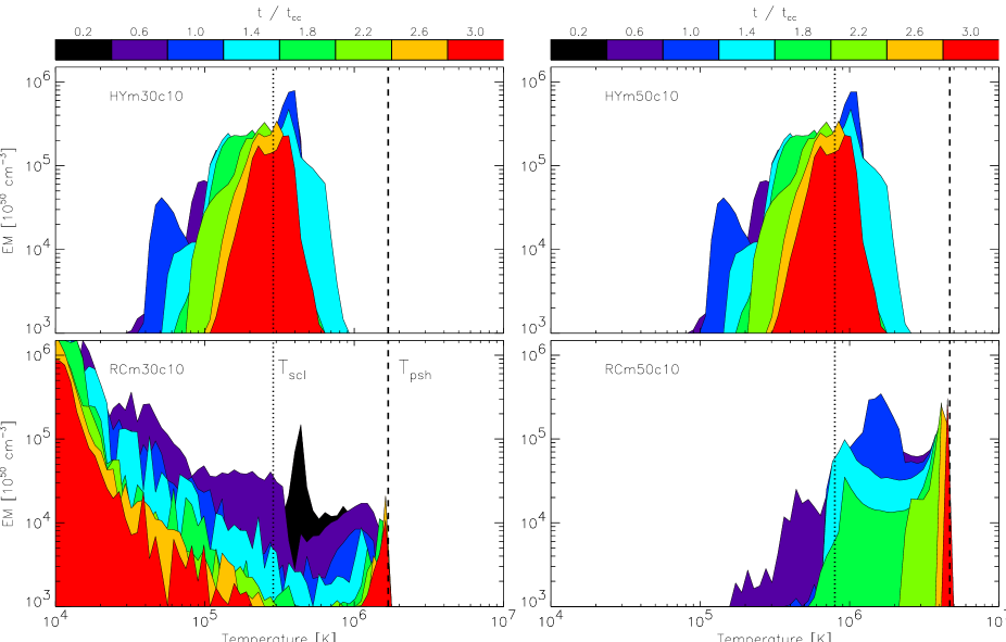
Figure 1: Evolution of the EM($T$) distributions of the cloud for ${\cal M}=30$ (left panels) and ${\cal M}=50$ (right panels) cases; upper panels show the result for models without thermal conduction and radiation (HY models), lower panels for models with both effects (RC models). The EM($T$) distributions are sampled every $0.4\leavevmode\nobreak\ \tau_{\rm cc}$ since $t=0.2\leavevmode\nobreak\ \tau_{\rm cc}$. The time sequence follows the color codes as reported in the color bar. The temperatures of the shocked ambient medium ($T_{\rm psh}$, see Tab. 2) and of the shocked cloud medium assuming negligible thermal conduction ($T_{\rm scl}$, see text) are marked with vertical dashed and dotted lines, respectively.

We use the cloud tracer mentioned in Sect. 2 to identify zones whose content is the original cloud material by more than 90%. From these zones, we then derive the EM($T$) distribution of the cloud. Fig. 1 shows the cloud EM($T$) evolution for the ${\cal M}=30$ (left panels) and ${\cal M}=50$ (right panels) cases, either without thermal conduction and radiation (hereafter HY models; upper panels) or with both effects (hereafter RC models; lower panels). We show the EM($T$) distributions sampled at steps of $0.4\leavevmode\nobreak\ \tau_{\rm cc}$ since $t=0.2\leavevmode\nobreak\ \tau_{\rm cc}$.

Fig. 1 shows that, in HY models, the EM($T$) distribution of the cloud is steadily centered around the temperature of the shock transmitted into the cloud, $T_{\rm scl}\approx\beta T_{\rm psh}/\chi$, where $\beta\approx 1.7$ (see Paper I), $\chi=10$; we obtain $T_{\rm scl}\approx 0.3$ MK for ${\cal M}=30$ and $T_{\rm scl}\approx 0.8$ MK for ${\cal M}=50$ (see dotted lines in Fig. 1). The evolution of the EM($T$) distribution for ${\cal M}=30$ and for ${\cal M}=50$ cases is similar, according to the Mach-scaling (Klein et al. 1994, Paper I): it rapidly becomes quite broad, covering more than a decade in temperature around $T_{\rm scl}$; then, at late stages, it gets narrower.

The EM($T$) distribution obtained from RC models significantly changes, depending on which process is dominant. When the radiative losses dominate (RCm30c10; lower left panel in Fig. 1), the EM($T$) distribution below 1 MK evolves toward a steep power law (with negative index), drifting to the cold side due to the progressive cooling of the plasma. A small fraction of cloud material gradually thermalizes by conduction to the temperature of the surrounding medium, forming a small peak centered at $T_{\rm psh}$. Thus, at variance from pure hydrodynamics, the plasma splits into two separate thermal components: a cold dense core ($T<0.1$ MK, see Paper I) and a hot diluted corona ($T\approx T_{\rm psh}=1.7$ MK).

In the conduction-dominated Mach 50 case (RCm50c10; lower right panel in Fig. 1), the EM($T$) distribution is initially broad and centered at the temperature of the shock transmitted into the cloud, $T_{\rm scl}$; then its maximum gradually shifts to higher and higher temperatures up to $T_{\rm psh}\sim 4.7$ MK getting more peaked, due to the thermalization of the cloud material to $T_{\rm psh}$.

3.2 X-ray emission

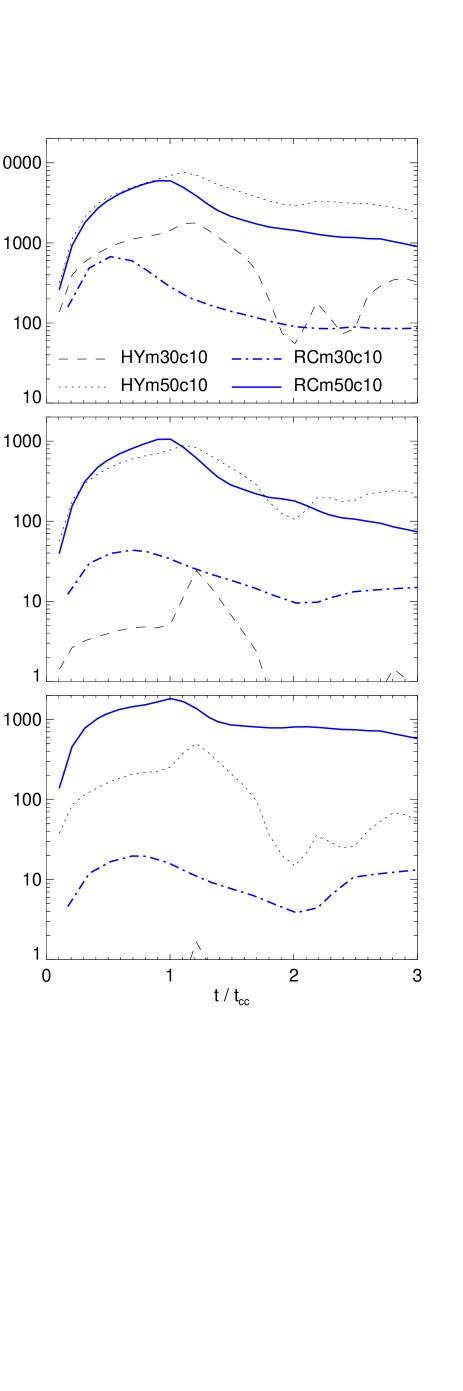
Figure 2: X-ray light curve of the cloud in the $[0.1-10]$ keV (top panel), $[0.3-0.5]$ keV (middle panel), and $[0.5-1.0]$ keV (bottom panel) bands of the shocked cloud derived for the ${\cal M}=30$ and ${\cal M}=50$ shock cases with (RC models) or without (HY models) thermal conduction and radiative cooling.

Fig. 2 shows the cloud X-ray light curves in the broad $[0.1-10]$ keV band and in the $[0.3-0.5]$ keV, and $[0.5-1.0]$ keV bands typically selected for the analysis of evolved SNR shock-cloud interactions (see, for instance, Miceli et al. 2005). The figure shows the X-ray luminosity, $L_{\rm X}$, of the shocked cloud only and does not consider the contribution originating from the shocked ambient medium surrounding the cloud. As expected, $L_{\rm X}$ is larger in the hotter ${\cal M}=50$ case than in the ${\cal M}=30$ case in all the energy bands and in both HY and RC models. In all the cases, the X-ray luminosity of the shocked cloud reaches its maximum quite early, around $t\sim\tau_{\rm cc}$, and then decreases (even by one order of magnitude, for instance, in HYm50c10 in the $[0.3-0.5]$ keV band); therefore, in the X-ray band, shocked interstellar gas clouds will be preferentially visible during the early phases of the shock-cloud collision.

We now discuss in detail the evolution of the cloud morphology as detected in the X-ray band. We expect the richest scenario from the hottest ${\cal M}=50$ case. Fig. 3 shows 2-D sections in the $(x,z)$ plane of the mass density distribution, $\rho$, the temperature, $T$, and the X-ray flux in the $[0.1-10]$ keV band, $F_{\rm X}$, derived from HYm50c10 and RCm50c10 models at $t=1.2\leavevmode\nobreak\ \tau_{\rm cc}$, just after the maximum luminosity of the cloud (see Fig. 2). The maps of $\rho$ and $F_{\rm X}$ are in log scale to highlight structures with very different density and X-ray fluxes.

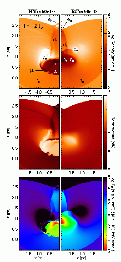
Figure 3: 2-D sections in the $(x,z)$ plane of the mass density distribution (gm cm^-3; top panels) in log scale, temperature (MK; middle panels), and X-ray emission in the $[0.1-10]$ keV band (erg s^-1; bottom panels), in log scale, derived from runs HYm50c10 (left panels) and RCm50c10 (right panels) at $t=1.2\leavevmode\nobreak\ \tau_{\rm cc}$. Labeled regions in the upper panels are discussed in the text.

At this stage of evolution, the whole cloud material has already been shocked. The size of the cloud ($\;\lower 4.0pt\hbox{${\buildrel\displaystyle<\over{\sim}}$}\,1$ pc) is smaller than that of the original unshocked cloud ($2\leavevmode\nobreak\ r_{\rm cl}=2$ pc) due to the cloud compression. The core of the cloud is a high density region ($a_{\rm H}$ and $a_{\rm R}$, see upper panel in Fig. 3) where primary and reverse shocks transmitted into the cloud are colliding (see also Paper I). A low density region ($c_{\rm H}$ and $c_{\rm R}$) due to a large vortex ring has developed just behind the cloud. In HYm50c10, hydrodynamic instabilities are developing at the cloud boundaries: the combined effect of instabilities and shocks transmitted into the cloud leads to unstable high-density regions at the cloud boundaries ($g_{\rm H}$). In RCm50c10, the thermal conduction suppresses the instabilities and leads to smooth gradients of density and temperature from the inner part of the cloud to the ambient medium. In both cases, the global forward shock has converged on the symmetry axis ($z$-axis), and undergoes a conical self-reflection, forming the primary Mach reflected shocks ($d_{\rm H}$ and $d_{\rm R}$) and the stem bulge at the base of the secondary vortex sheets near the symmetry axis ($e_{\rm H}$ and $e_{\rm R}$; see Fig. 6 in Poludnenko et al. 2002 for a detailed description of the flow structures developing during the shock-cloud interaction). The reflected bow shock is visible as a curved region extending into the shocked ISM right below and along the sides of the cloud (regions $f_{\rm H}$ and $f_{\rm R}$).

The comparison between upper and lower panels of Fig. 3 shows that, in both models, the region with the highest X-ray flux is in the core of the cloud (regions $a_{\rm H}$ and $a_{\rm R}$). In HYm50c10, the X-ray image of the shocked cloud has a very sharp boundary and even the hydrodynamic instabilities at the cloud boundary are clearly marked in the X-rays (region $b_{\rm H}$); high X-ray flux also originates from the unstable high-density regions at the cloud boundaries (region $g_{\rm H}$). In RCm50c10, instead, the emission from region $b_{\rm R}$ is more diffuse, varying smoothly in the radial direction from the center of the cloud. Fig. 3 also shows that the X-ray emission density in the reflected bow shock (regions $f_{\rm H}$ and $f_{\rm R}$) and in the primary Mach reflected shocks ($d_{\rm H}$ and $d_{\rm R}$) is slightly higher (by a factor $\sim 2$ in HYm50c10, and by a factor $\sim 4$ in RCm50c10) than that of the post-shock ambient medium not involved in the shock-cloud interaction. On the other hand, the low density region ($c_{\rm H}$ and $c_{\rm R}$) and the stem bulge ($e_{\rm H}$ and $e_{\rm R}$) are characterized by very low X-ray emission.

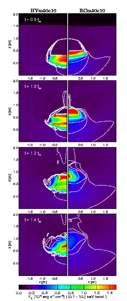
Figure 4: X-ray images in the [$0.1-10$] keV band in linear scale derived from models HYm50c10 (left panels) and RCm50c10 (right panels) at the labeled times. Contours are the mass density distribution in the $(x,z)$ plane, corresponding to $\log\rho\leavevmode\nobreak\ \mbox{(gm cm${}^{-3}$)}=-23.9,\leavevmode\nobreak\ -23.7,\leavevmode\nobreak\ -23.5,\leavevmode\nobreak\ -23.3$. Regions “1” and “2” in the third row originate from regions $a_{\rm H}$ and $g_{\rm H}$, respectively, shown in Fig. 3.

Fig. 4 shows the map of X-ray emission in the $[0.1-10]$ keV band (in linear scale) integrated over 10 pc along the LoS (see Sect. 2.2) for HYm50c10 and RCm50c10 at four selected epochs around the time of the maximum cloud X-ray luminosity (see Fig. 2). The superimposed contours are the mass density distribution (in log scale) in the $(x,z)$ plane. The third row of plots corresponds to the time of Fig. 3 ($t=1.2\leavevmode\nobreak\ \tau_{cc}$). The highest integrated emission originates in the core of the shocked cloud in both models; two separate high-emission regions are visible in HYm50c10 around $t=\tau_{\rm cc}$: the upper region (labeled “1” in the third row of Fig. 4) is the high-density region $a_{\rm H}$ discussed above (see Fig. 3), whereas the lower one (region labeled “2”) originates from the integration along the LoS of the emission of high-density unstable regions at the cloud boundary (region $g_{\rm H}$ in the upper panel in Fig. 3). In HYm50c10, the hydrodynamic instabilities are no longer clearly distinguishable after integration along the LoS. In RCm50c10, the brightest portion of the shocked cloud corresponds to the high-density region ($a_{\rm R}$), appears significantly smaller and shorter-lived than in HYm50c10 and, in general, the cloud surface brightness rapidly approaches the values of the surrounding medium. The reflected bow shock (regions $f_{\rm H}$ and $f_{\rm R}$) and the primary Mach reflected shocks (regions $d_{\rm H}$ and $d_{\rm R}$) have a surface brightness more than a decade lower than that of the cloud core.

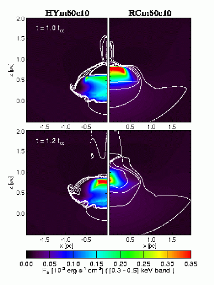
Figure 5: As in Fig. 4 for the two labeled times and for the [$0.3-0.5$] keV band.

Fig. 5 shows that the highest emission comes from the core of the shocked cloud (regions $a_{\rm H}$ and $a_{\rm R}$) in the $[0.3-0.5]$ keV band, and is maximum at $t\approx\tau_{\rm cc}$ for RCm50c10 and at $\approx 1.2\leavevmode\nobreak\ \tau_{\rm cc}$ for HYm50c10. In model RCm50c10, the cloud fades out earlier than in HYm50c10 because of the dissipation by thermal conduction.

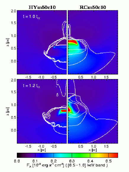
Figure 6: As in Fig. 5 for the [$0.5-1.0$] keV band.

In the higher energy $[0.5-1.0]$ keV band, shown in Fig. 6, the shocked cloud is bright only around $\tau_{\rm cc}$. In particular, in HYm50c10, a small fraction of the cloud (the high-density region $a_{\rm H}$; see Fig. 3) has significant emission only for a very short time around $1.2\leavevmode\nobreak\ \tau_{\rm cc}$ (see Fig. 6). In RCm50c10, instead, the X-ray image of the cloud appears more extended and diffuse than in HYm50c10, and the cloud is already visible at $t=0.2\leavevmode\nobreak\ \tau_{\rm cc}$ (not shown in Fig. 6) and remains bright until $t=1.4\leavevmode\nobreak\ \tau_{\rm cc}$. This larger-lasting emission is due to the increased cloud X-ray emission at higher energies, determined by the thermal conduction that heats the cloud material to higher temperatures.

For further details on the evolution of the X-ray emission in the three bands selected, see the on-line material.

3.3 Median energy of X-ray photons

The map of the median energy of X-ray photons (hereafter the MPE map) is a practical tool to convey at the same time both spatial and spectral information on the emitting plasma at high resolution (Hong et al. 2004; see also Miceli et al. 2005).

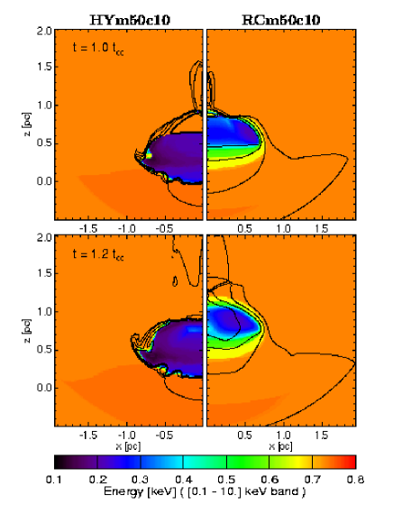
Figure 7: Median photons energy maps in the $[0.1-10]$ keV band derived for HYm50c10 (left panels) and RCm50c10 (right panels) at the labeled times. Contour plots as in Fig. 4.

Fig. 7 shows the model MPE maps at the times of Figs. 5 and 6 obtained from the spectra synthesized in the [$0.1-10$] keV band (see Sect. 2.2). By comparing the MPE maps in Fig. 7 with the X-ray images in Fig. 4, we note that, during the whole evolution, the X-ray emission is high where the median photon energy ${\overline{\cal E}}\,$ is low. This result is evident in the ${\overline{\cal E}}\,$ versus $F_{\rm X}$ scatter plot derived for both HYm50c10 and RCm50c10 models at $t=1.2\leavevmode\nobreak\ \tau_{\rm cc}$ (Fig. 8). In fact, most of the brightest pixels are in the shocked cloud, i.e. plasma with temperature lower than that of the shocked surrounding medium. Fig. 8 also shows that, for $F_{\rm X}>0.5\times 10^{-3}$ erg s^-1 cm^-2, ${\overline{\cal E}}\,$ increases with $F_{\rm X}$ indicating that the cloud plasma is far away from pressure equilibrium.

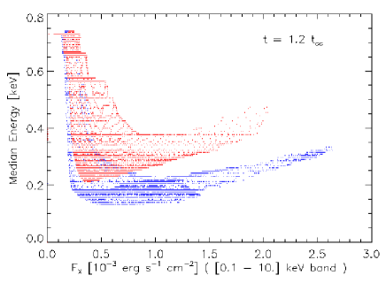
Figure 8: Median photon energy, ${\overline{\cal E}}\,$, versus X-ray flux in the $[0.1-10]$ keV band, $F_{\rm X}$, scatter plot derived for HYm50c10 (blue) and RCm50c10 (red) at $t=1.2\leavevmode\nobreak\ \tau_{\rm cc}$.

Fig. 7 also shows that, in HYm50c10, the low ${\overline{\cal E}}\,$ region is rather uniform with ${\overline{\cal E}}\,\approx 0.2$ keV, and its boundaries are sharp. In model RCm50c10, instead, the thermal conduction smoothes the energy gradient: in the low ${\overline{\cal E}}\,$ region, ${\overline{\cal E}}\,$ increases smoothly from the cloud center to the surrounding medium. The minimum ${\overline{\cal E}}\,$ value is higher ($\sim 0.3$ keV) than that in HYm50c10 ($\sim 0.2$ keV) because of the heat conducted into the cloud.

4 Discussion and conclusion

We derived the X-ray emission predicted by hydrodynamic modeling of the interaction of a SNR shock wave with an interstellar gas cloud. Our forward modeling allows us to link model results to observable quantities and to investigate the observability of features predicted by models.

Our analysis has shown that the morphology of the X-ray emitting structures is significantly different from the morphology of the flow structures originating from the shock-cloud interaction. For instance, the complex pattern of shocks (e.g. external reverse bow shock, shocks transmitted into the cloud, Mach reflected shocks at the symmetry axis, etc.) as well as other flow structures (e.g. hydrodynamic instabilities, the stem bulge at the base of the secondary vortex sheets near the symmetry axis, etc.) caused by the shock-cloud collision are visible in the density maps, but they are never clearly distinguishable in X-ray images (cf. upper panel in Fig. 3 and third row of Fig. 4 at $t=1.2\leavevmode\nobreak\ \tau_{cc}$). Indeed, the morphology of the X-ray emitting structures appears quite simple in all the cases examined. The largest contribution to the X-ray emission originates from the core of the cloud where primary and reverse shocks transmitted into the cloud collide. The bright core is surrounded by a diffuse and faint region associated with the outer portion of the cloud. The X-ray emission varies smoothly in the radial direction from the bright core to the surrounding medium.

The hydrodynamic instabilities, developing at the cloud boundaries in models without thermal conduction, are never clearly visible in the X-ray band because faint and washed out by integration along the LoS. On the other hand, the interaction of the instabilities with shocks transmitted into the cloud produces a bright region with luminosity comparable to that of the cloud core (region labeled “2” in Fig. 4). At variance with models including thermal conduction, therefore, in HY models two separate bright regions develop inside the shocked cloud. This has an important implication on the diagnostics. In fact, in Paper I, we have shown that the thermal conduction is very effective in suppressing hydrodynamic instabilities: the evidence of these instabilities during the shock-cloud interaction would be an indication that the thermal conduction is strongly inhibited (for instance by an ambient magnetic field). Our analysis points out that, unfortunately, the X-ray band cannot give strong indications about hydrodynamic instabilities in any case.

Our modeling has also shown that shocked interstellar gas clouds reach their maximum X-ray luminosity around $t\sim\tau_{\rm cc}$. The size of the bright region in X-ray maps varies during the shock-cloud interaction: the maximum extension is reached at epochs $<\tau_{\rm cc}$ and is always significantly smaller than the original cloud diameter. The light curve of the shocked cloud and the evolution of the bright region indicate that shocked clouds are expected to be preferentially observed in the X-rays during the early phases of shock-cloud collision.

As an example, in the ${\cal M}=50$ shock case considered here, the shocked cloud has total luminosity in the $[0.5-1.0]$ keV band $L_{\rm X}\;\lower 4.0pt\hbox{${\buildrel\displaystyle>\over{\sim}}$}\,10^{33}$ erg s^-1 during the period $0.4\leavevmode\nobreak\ \tau_{\rm cc}<t<1.3\leavevmode\nobreak\ \tau_{\rm cc}$ (see Fig. 2). Since the XMM-Newton/EPIC-MOS sensitivity limit in the $[0.5-2.0]$ keV band is $F_{\rm epic}\approx 10^{-14}$ erg cm^-2 s^-1 for an exposure time of $10^{4}$ s (Watson et al. 2001), our analysis suggests that such emission should be detectable as far as $\approx 30$ kpc.

The modeling shows that thermal conduction and radiative cooling can lead to two different gas phases emitting in different energy bands: a cooling dominated core which ultimately fragments into cold, dense, and compact filaments emitting at low energies (e.g. optical band), and a hot thermally conducting corona emitting at high energies (e.g. soft X-rays). Both phases are clearly present in the ${\cal M}=30$ case but only the hot one in the ${\cal M}=50$ case because thermal conduction is highly effective. As an implication, we expect that the X-ray emission morphology and spectrum of the bright cloud region should be sensitive to thermal conduction effects. In fact, thermal conduction makes the X-ray bright region smaller, more diffuse, and shorter-lived than that expected when thermal conduction is neglected. Also, we found that the median photons energy of the bright region is higher in models with thermal conduction. As a final diagnostic consideration, we note that observing smooth gradients of emission and median photon energy would indicate that the thermal conduction is efficient.

The results presented here illustrate the X-ray radiation emitted during the shock-cloud collision. Our analysis provides a way: 1) to link the features expected to emit X-rays with plasma structures originating during the shock-cloud collision, and 2) to investigate the effects on the X-ray emission of the different physical processes at work. These results will be a guide for the interpretation of X-ray observations of middle-aged X-ray SNR shells whose morphology is affected by ISM inhomogeneities (e.g. the Cygnus Loop, the Vela SNR, G272.2-3.2, etc.). However, a more direct comparison of model results with supernova remnant X-ray observations requires to include instrumental response and sensitivity and ISM absorption. In a companion paper (Orlando et al., in preparation), we will step forward to investigate in detail the direct diagnostics and comparison with the data collected with the latest X-ray instruments (i.e. Chandra, XMM-Newton).