Luminosity Function of Faint Globular Clusters in M87

Abstract

We present the luminosity function to very faint magnitudes for the globular clusters in M87, based on a 30 orbit Hubble Space Telescope (HST) WFPC2 imaging program. The very deep images and corresponding improved false source rejection allow us to probe the mass function further beyond the turnover than has been done before. We compare our luminosity function to those that have been observed in the past, and confirm the similarity of the turnover luminosity between M87 and the Milky Way. We also find with high statistical significance that the M87 luminosity function is broader than that of the Milky Way. We discuss how determining the mass function of the cluster system to low masses can constrain theoretical models of the dynamical evolution of globular cluster systems. Our mass function is consistent with the dependence of mass loss on the initial cluster mass given by classical evaporation, and somewhat inconsistent with newer proposals that have a shallower mass dependence. In addition, the rate of mass loss is consistent with standard evaporation models, and not with the much higher rates proposed by some recent studies of very young cluster systems. We also find that the mass-size relation has very little slope, indicating that there is almost no increase in the size of a cluster with increasing mass.

1 Introduction

The dynamical evolution of globular clusters has long been the subject of many theoretical studies, including a number of recent papers utilizing state of the art simulations (e.g. Baumgardt & Makino, 2003, and references therein). These studies find that mass loss due to two body relaxation and the resulting evaporation is the primary mechanism for the destruction of globular clusters. Only those clusters with disruption timescales similar to or less than a Hubble time will be significantly changed by this evolution over their lifetimes. As evaporation causes clusters to lose mass at a fairly constant rate, the disruption timescale is directly related to the initial mass of the cluster. Therefore, the clusters with the lowest initial masses should constrain the form of this evolution most strongly. These low mass clusters have lower luminosities, which makes them difficult to observe in other galaxies. For the Milky Way, where finding lower luminosity clusters is not as difficult, the small total number of clusters prevents any results from being statistically strong. What is needed to provide constraints on the models of the dynamical evolution of globular clusters is a system which has both large numbers, and observations that reach low masses with a high degree of accuracy and reliability.

In this paper, we present results from new, very deep HST images of M87 that achieves these goals of depth and large numbers of globular clusters. In §2, we present the data and explain the procedures used to measure the globular clusters in M87. We present our luminosity function in §3, and compare it to other deep luminosity functions that have been previously published. We show our mass function, and show the constraints it gives for theoretical models of globular cluster evolution in §4. Finally, we present our conclusions in §5.

2 Observations and Reductions

2.1 Observations and Data

The center of M87 was imaged with the WFPC2 as part of a 30 orbit program (Baltz et al., 2004) in May and June of 2001. During each orbit, four exposures totalling 1040s were taken in the F814W filter, with a single matching 400s exposure in the F606W filter. The four F814W images were dithered by half pixel steps to allow for the images to be interlaced directly into a 2x2 grid. Average images were created from the final full data set by stacking the images, after they had been sinc-interpolated to a common origin. The images from day 12 were excluded from this step as they had more jitter than the other images. This combination creates images that have total exposure times of $30160$s for F814W, and $11600$s for F606W.

Cluster detection was performed separately on the images for each filter using Source Extractor (Bertin & Arnouts, 1996). As we are imaging the center of the galaxy, the galaxy profile is steep. Because the main source of noise in the image is from the variation in the number of photons detected from the galaxy light, this steep profile creates a rapid change in the noise level across the images. To prevent the change in noise from altering how clusters are detected at different distances from the galaxy, we created an image to model the background level of the galaxy itself. This was done by median filtering the image with a box larger than the size of any of the globular cluster features. As the radii of the largest clusters can be up to 20 pixels, we use a filter box of 50 x 50 pixels. This background image was used to weight the detection threshold, which helps minimize radial variations in our object detection.

2.2 Object Selection and Completeness

Since the faint end of the observed GCLF is sensitive to the contamination of objects that are not globular clusters, we want to ensure that we remove as many of these objects as possible. The majority of the very faintest objects detected are likely to be simply peaks in the variation of the background. As the background subtracted image histograms are symmetric about zero, we expect that the magnitude and frequency of these variations are the same between peaks and valleys. Therefore, by inverting the sign of the data images (simply multiplying by $-1$), and searching on these images, we can determine how many candidate clusters are caused by the variations in the background level. Based on these tests, we chose detection thresholds of $3\sigma$ with a minimum object size of 2 pixels. Although it is tempting to push this lower to increase the completion at fainter magnitudes, below this limit the increase in the number of objects detected on the data image is closely matched by an increase in the number of objects detected on the inverted image. This suggests that we are not reliably adding new real clusters to our sample.

In addition to these false clusters, we also expect to have a contribution from faint galaxies behind M87. This contribution can be estimated by measuring how many objects we find with our settings on very deep HST images like those of the Hubble Deep Field (Williams et al., 1996). The detection efficiency for faint extended objects is very sensitive to the signal to noise ratio of the image. This required us to degrade the quality of the HDF image to match the average variance of our images.

To help remove as many contaminating objects as possible, we demand that two requirements be met before an object was determined to be a valid globular cluster. The first requirement is that all globular cluster candidates must be detected in both filters. This removes a significant portion of the false clusters, as well as a few of the HDF objects. By further requiring that all candidates have a final $V-I$ color between 0.5 and 1.7, we exclude almost all of the remaining background sources and false clusters. As shown in Table 1, each of these cuts removes approximately the same number of clusters from both the observed and false sets which suggests that these cuts preserve the real clusters, and only remove objects that are not globular clusters.

With the detection parameters set, we next used model clusters of known flux to determine the completeness of our sample. All of the model clusters were generated from King model profiles with a fixed concentration of 1.26 at eight tidal radius steps evenly spaced between 2 and 16 pixels. These templates were then scaled to form a grid in magnitude and size, with F814W and F606W apparent magnitudes spaced every 0.5 magnitude between 20 and 28 magnitude. This range of radii and magnitudes was chosen to cover the properties of the real clusters in our data sample.

For each combination of magnitude and tidal radius, 150 copies of the template were randomly placed on the background subtracted images. Source Extractor was then used to find these objects with the same detection parameters as were used on the data image. By measuring the rate at which the templates are recovered, we can determine how complete our data sample is. Because the change in the completeness did not vary much for template clusters of different sizes, the final completeness is found by simply averaging the results for all radii together.

As the detection process is sensitive to the background uncertainty, the completeness limit becomes fainter as the distance from the center of the galaxy increases. To take advantage of this increased sensitivity, we divided our sample into two radial bins with equal numbers of clusters in each. This gives bins that have rages of projected galactocentric distances from $1.1$kpc to $4.4$kpc, and from $4.4$kpc to $9.0$kpc. The completeness for each bin was then calculated based only on the templates that fell within that bin.

Our requirement that clusters be detected in both the F814W and F606W filters also influences the final completeness curves, which are simply the product of the two completenesses for each filter. For clusters that are bright enough in both filters to be reliably detected, this has no effect. Because of the depth of our data, this limit extends to $V\sim 25$, much fainter than the turnover of the globular cluster luminosity function. For clusters fainter than this, the color dependence begins to exclude the bluest clusters. The resulting 50% completeness limit for our samples in the two radius bins is $V_{inner}=25.07+0.62(V-I)$ and $V_{outer}=25.27+0.63(V-I)$.

Figure 1 shows the final observed color magnitude diagram, based on the photometric calibration discussed in section 2.3. The left panel shows all objects detected in our data image, with the right panel showing the detections from the HDF background field, as well as from the image background fluctuations. It is clear from this plot that with the cuts that we have applied, nearly all of the contaminating objects are removed from the sample, leaving a sample that is composed overwhelmingly by globular clusters.

2.3 Aperture Correction and Photometric Calibration

In addition to allowing us to measure the completeness of our detection process, our templates also provide a direct way to measure the aperture corrections for our clusters. The globular clusters on our image are extended objects, and as such, fixed apertures may not measure all the light equally well for all clusters. We can estimate what the aperture correction should be for our clusters by comparing the measured magnitudes for the templates to the known magnitude with which they were created.

All photometry was done using two fixed apertures of 2 and 4 pixels. We were then able to construct a parameter to estimate how extended the clusters are by taking the difference between these two magnitudes. By taking the median values for this parameter, the outer aperture magnitude, and the required aperture correction for each combination of template size and input magnitude, we were able to create a mesh of values that can be used to calibrate the real clusters. For each cluster, the aperture correction was calculated by finding the value at the mesh point that most closely matched the observed outer aperture magnitude and magnitude difference. This method works well for most of the observed clusters, although at faint magnitudes, the scatter in our measured parameters increases, and the decrease in the number of templates recovered allows this increased scatter to propagate to the mesh point values. By passing the template clusters through this procedure as well as the real clusters, we were able to determine that the aperture correction introduces an uncertainty of 0.1 magnitudes into the final magnitudes, similar to what is found in other HST studies of extragalactic globular clusters (e.g. Kundu et al., 1999). As both filters are affected equally by this uncertainty, the calculated colors are not changed.

We used the zeropoints and color corrections listed in Holtzman et al. (1995) to convert the aperture corrected instrumental magnitudes into standard V and I magnitudes. The extinction for M87 from Schlegel et al. (1998) was also applied to our measurements. Finally, the standard 0.1 magnitude aperture correction was applied to the final magnitude to correct for the light that is lost to scattering by the WFPC2 optics. To confirm that our magnitudes match those previously published for the M87 globular clusters, we compared our final magnitudes to those presented by Kundu et al. (1999) for the 346 clusters that are common to both samples. The average differences between our magnitudes for the clusters are $\langle V-V_{Kundu}\rangle=-0.042$ and $\langle I-I_{Kundu}\rangle=-0.021$, well within our $0.1$ magnitude uncertainty due to the aperture correction.

The color magnitude diagram for the objects we consider globular clusters is presented in figure 2. This sample contains only the points that fall within our color cuts, as well as to detections that are above the 50% completeness limit. We have also overplotted a line showing the weak trend between the median brightness of cluster as a function of color, $V\propto 29(V-I)$. This difference follows naturally from stellar population models, which predict that the lower metallicity blue clusters will have a smaller $M/L_{V}$ than the higher metallicity red ones (see discussion in Kundu et al., 1999, and references therein). This also creates a spread in the $M/L_{V}$ ratios for the clusters, which tends to broaden the luminosity function.

2.4 Size Measurements

The half-light radii for each cluster was measured using Source Extractor. As shown in Figure 3, the measured range of half-light radii for the real clusters appears to be generally constant over all magnitudes. This suggests that any biases in our measurements of the cluster sizes must be fairly small. To confirm this, we generated a random sample that is evenly populated over the observed range of $V-I$ color, $V$ magnitude and $r_{half}$ sizes. At each point, we calculated the completeness as a function of these three parameters. The observed half-light radius was included by keeping the completeness results separated by the input template sizes. We then assigned that size template the median half-light radius that was found during the template recovery.

Using this sample, we can investigate how strongly we expect the real cluster sample to be biased. The photometric errors for the faintest clusters should tend to decrease the measured half-light radius. In addition, the low surface brightness of large faint clusters may also cause such clusters to not be detected, which will also decrease the average size observed for faint clusters. We selected only those clusters that had calculated completeness greater than 50%. The median half-light radius was then found for bins spaced equally in $\log(L)$ for both the random sample and the sample of real clusters, with errors determined via bootstrapping. Linear fits were then performed on the values of $\log(L)$ and $\log(r_{half})$. These best fitting lines, as well as the binned data are shown in Figure 3. We find that the random sample is best fit by a relation $r_{half}\propto L^{0.01}$. This indicates that we are not significantly biased against large, faint clusters, and that the change in size due to errors must also be small.

For the real clusters, the trend is not much stronger, with $r_{half}\propto L^{0.04}$. The increased scatter compared to the random sample is likely due to the real distribution of cluster concentrations. This introduces a distribution of half-light radii that is larger than that in our random sample, as our use of only a single concentration value in our templates ignores any such variation. The weak observed trend shows clearly that the median half-light radius of globular clusters changes very little over the magnitude range that we observe. This result is similar to what has been observed for the Milky Way system (e.g. Ashman & Zepf, 1998), as well as for young globular cluster systems in other galaxies (Zepf et al., 1999; Larsen, 2004). The similarity between both the young and old cluster systems suggests that this trend arises during cluster formation, and as such, is an important constraint on formation models for globular clusters (see Ashman & Zepf, 2001, and references therein).

3 Luminosity Function

The luminosity function histogram (figure 4) was created by binning each cluster by a weight factor, defined to be $W=(\textup{completeness}(V,V-I))^{-1}$. The error for each bin is then $\langle W\rangle\sqrt{N}$, where $N$ is the number of clusters actually detected in the bin, and $\langle W\rangle$ is the average of the weight factors for the clusters in the bin. The effect of the contamination from false detections of background noise, as well as from background galaxies, are weighted in the same way, and subtracted from the bin that they would fall in if they were real clusters. This corrects our luminosity function both for any real clusters that we may have missed, as well as for any objects detected that are not real globular clusters.

For each of our two radial bins, we created separate luminosity functions in the same way as for the entire sample. These two luminosity functions are shown along with the median completeness for each sample in figure 5. By comparing these luminosity functions for the two bins, we can check that any radial trend, including from our completeness correction, does not influence the final luminosity function. This comparison was done on the unbinned distributions by using an F-test to check that the variances are the same between the two bins, and a t-test to check that the turnover in the luminosity function is in the same location. For both tests, we use the hypothesis that the distributions are the same, and find that we can accept the hypothesis for both tests (F-test p-value = 0.24; t-test p-value = 0.94), indicating no significant difference between the luminosity functions at our two radii.

Since the two radial bins are similar, we can work with the final luminosity function at all radii, and compare this final luminosity function to those that have been presented before for globular cluster systems. The two most important comparisons are to previous results for the M87 globular clusters and to the Galactic globular cluster system. For M87, the most complete previous study of the globular cluster luminosity function is by Kundu et al. (1999). They fit a Gaussian to their binned luminosity function, finding that $\langle V\rangle=23.67$ with $\sigma=1.39$. Repeating this for our luminosity function yields similar results, with $\langle V\rangle=23.60$ and $\sigma=1.42$. We can also test how well the unbinned distributions match, again using an F-test and a t-test to check the agreement of the variances and turnover location. The F-test allows us to accept our hypothesis (p-value = 0.26), indicating that the variances of the two distributions are consistent with each other. The t-test also allows allows us to accept the hypothesis (p-value = 0.94), suggesting that the location of the turnover is the same for both as well. The combination of these two results leads to the conclusion that our luminosity function is consistent with that previously published for M87.

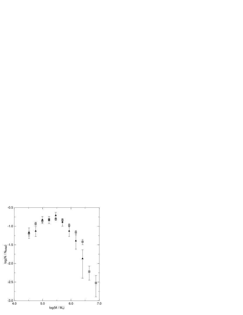
Figure 6: Comparison of our globular cluster mass function for M87 (squares) to the mass function of the Milky Way (triangles), based on the globular cluster catalog of Harris (1996).

We can repeat this procedure for the Milky Way clusters, and see if this luminosity function also matches. We used the catalog of galactic globular clusters of Harris (1996), and adopted a distance to M87 of 16 Mpc (Macri et al., 1999). We find that a Gaussian fit to the binned Milky Way luminosity function yields $\langle V\rangle=23.70$ and $\sigma=1.18$. Running the same tests as above with the same hypotheses, we can conclude that the turnovers are the same (t-test p-value = 0.99), but that the variances are significantly different (F-test p-value = $8\times 10^{-3}$). This can be seen in figure 6, which illustrates that the Milky Way distribution is significantly narrower.

This difference in the dispersions may be related to the differences in the cluster color distributions between the galaxies. M87 has a strongly bimodal color distribution, with roughly equal numbers of red and blue clusters. These two populations serve to spread out the total luminosity function, as the blue population tends to be brighter than the red ($\langle V_{blue}\rangle=23.27$, $\langle V_{red}\rangle=23.62$). This separation serves to increase the total luminosity function dispersion. The shape of the luminosity function remains a smooth Gaussian, as the dispersions of both of these populations are larger than the separation in the means. Because the blue population dominates the Milky Way system, there is correspondingly little effect from the spread of cluster colors on the dispersion of the luminosity function.

4 Mass function

As our data probe well beyond the turnover of the GCLF, we can use it to gauge how well current cluster evolution models track the observations. Theory predicts that dynamical evolution is the dominant factor in the shape of the current luminosity function. To compare to theoretical models, we need to convert the luminosities into masses. We adopt a $M/L$ ratio of 3 based on work on the structural parameters (Waters & Zepf, 2006) as our fiducial value. Changes in this value do not change the relative fit quality between the observed mass function and the theoretical models that we compare to. However, changes will alter the mass loss rates that we calculate from our data, such that all of the rates that we calculate should be scaled by a factor $(M/L)/3$.

The models that we consider are of the general form of $\dot{M}=\nu(M)M$ where $\nu(M)$ is the decay rate of a cluster with mass $M$ (cf. Fall & Zhang, 2001). This form is useful, as it allows a number of previously published evolution models to be analyzed in the same way. Generally, these models have $\nu(M)\propto M^{-\gamma}$, or $\dot{M}\propto M^{1-\gamma}$. The first such model we consider is a standard evaporation model in which $\dot{M}\propto M^{0}$, such as the one described by Fall & Zhang (2001). We also consider a simplified form of the evaporation model derived by Baumgardt & Makino (2003) from their analysis of N-body simulations of globular clusters. Briefly, their result was that the disruption timescale for clusters scales as $T_{dis}\propto M^{0.75}$, which we can convert into a mass derivative by noting that $\int_{M_{0}}^{0}\dot{M}^{-1}dM=T_{dis}$, and then solving this equation for a mass loss rate as defined above. This gives a final derivative of $\dot{M}\propto M^{0.25}$. Finally, we investigate the numerical fit to this result that is presented in Lamers et al. (2005). They also present a disruption time, which they solve for in terms of the cluster mass and local density. We can convert this disruption time, $T_{dis}\propto M^{0.62}$, into a mass loss rate $\dot{M}\propto M^{0.38}$.

As these models only evolve single clusters, we need to create a population of globular clusters to compare with the observed mass function. We used two initial mass function models that have been used to fit the high mass globular cluster mass function before. As these clusters are not affected greatly by dynamical evolution, they are assumed to trace the initial mass function closely. The first of these functions is a straight forward power law, $dN=M^{-\beta}dM$, with $\beta\sim 1.8$, as suggested by studies of young star clusters (e.g. Zhang & Fall, 1999; Whitmore, 2003). The second is a more complex model designed to more accurately fit the observed number of high mass clusters in other galaxies, and as such, allows that data to influence the fitting more than it does in the case of the power law. We chose the model for the M87 globular cluster system presented by Burkert & Smith (2000), where $dN=M^{-3/2}\exp\left(\frac{-M}{M_{C}}\right)dM$ with $\log(M_{C})=6.4$, based on their fit to the bright M87 data and our adopted mass to light ratio.

To determine how well these models fit the observed mass function, we first generated a sample of test clusters with masses randomly drawn from a uniform distribution in $\log(M)$. Each test cluster was then assigned a weight calculated from the relative number of clusters expected from the initial mass function. This ensures that we consider all possible masses equally, while keeping the number of test clusters reasonable. For each cluster in this sample, we used the differential equations above to let the cluster evolve to an age of 12 Gyr. After the entire sample had been evolved, it was binned to create the final theoretical mass function.

These theoretical mass functions were then fit to our observed data. We allowed the functions two free parameters: $k$, the coefficient of the mass loss differential equation, and the normalization of the initial mass function. The coefficient determines the rate at which the clusters evolve, with larger constants yielding faster mass loss and shorter lifetimes. For the evaporation model, this coefficient is simply the constant mass loss rate. The normalization is independent of the exact form of the evolution, as it merely sets the total number of clusters present before any evolution. We ignore stellar evolution and gravitational shocks in our models, as these processes dominate only the earliest parts of the lifetimes of clusters. Because of this, our values for $N$ assume that any losses due to these processes have already been included. We have also ignored the effects of dynamical friction, which would serve to decrease the observed number of high mass clusters. If we restrict the data only to clusters with mass less than $1\times 10^{6}$, then the differences between the initial mass functions are largely ignored, and the evolved mass function is nearly independent of the initial one. Without this restriction, the fits based on the Burkert & Smith (2000) initial mass function match the observed full data set better than the simple power law mass function due to the falloff that this mass function has at high masses.

Plots of the best fitting models are given in figure 5, with the corresponding parameters for these fits listed in table 2. The values of $k$ are given in units of $M_{\odot}\textup{Gyr}^{-1}$, and the values of $N$ give the number of initial clusters with masses between $\log(M)=5.5$ and $\log(M)=7$. As shown in figure 5, our data are better fit by the standard evaporation model than the other models we consider. However, the uncertainties for the lowest mass bins, where the leverage to distinguish between the models is strongest, are too large to allow us to conclusively rule out any model.

We then compare the best fitting mass loss coefficient $k$ for each of the various dynamical models to the prediction the models give for the mass loss rate. For the standard evaporation model, we adopt the mass loss rate $k=269\xi_{e}(G\bar{\rho})^{1/2}m\ln\Lambda$, presented by Fall & Zhang (2001), as they explicitly give this rate constant for their solution. Our simplification of the Baumgardt & Makino (2003) model makes it difficult to test that model. We can derive the expected rate from the Lamers et al. (2005) disruption time, which yields $k=\frac{\bar{\rho}^{1/2}}{0.62C_{env}}(10^{4})^{0.62}$. To compare these rates with our best fit values, we have assumed a constant density for all of our clusters based on the M87 mass profile from Vesperini et al. (2003), calculated at our median galactocentric distance ($R_{g}=4.4$kpc).

For the evaporation model, the best fitting mass loss rate is consistent with that expected from theoretical calculations. We find that the fit of the Lamers et al. (2005) model to our M87 data requires a value of $C_{env}=720$ in their notation, which is close to the value of $C_{env}=810$ they derive from the Baumgardt & Makino (2003) disruption time. Somewhat lower values of $C_{env}$, which yields a faster disruption timescale, can be accommodated by using lower mass to light ratios to convert the cluster luminosities into masses. However, even including any uncertainties in our mass to light ratio, our data are clearly inconsistent with some of the smallest values ($C_{env}\sim 300$) suggested by Lamers et al. (2005) based on their analysis of young cluster systems. This shows that mass loss rates for two-body processes in fully relaxed old clusters can not be extrapolated from unrelaxed young systems.

One further effect is that toward the end of a globular cluster’s lifetime, mass segregation has moved the lowest mass stars to the outer edges of the cluster. These low mass stars are then preferentially stripped from the cluster, as they are less tightly bound. This tends to decrease the $M/L$ ratio of the cluster at the end of its life, as these low mass stars contribute more mass to the cluster than light. Since the globular cluster mass function is based on observations of the cluster light, using a constant $M/L$ ratio for all clusters overestimates the mass of these faintest clusters. We may see evidence for this effect, as our lowest mass bin falls below all of the model predictions. Any correction for such a changing $M/L$ ratio will serve to spread our lowest mass bin to even lower masses, which will tend to bring the result into agreement with the predictions of the evaporation model.

5 Discussion

Previous studies have probed beyond the turnover of the globular cluster luminosity function, yet none have reached the same depth as our new luminosity function for M87. This new depth has allowed us to trace the effects of dynamical evolution down to clusters that are in the last few Gyr of their lifetime, where the effects of the mass loss are most severe. The superior resolution offered by the data has also allowed us to establish that the size distribution of globular clusters is largely independent of the cluster luminosity over the entire range we observe.

The differences in dispersion that we have observed between the luminosity functions for M87 and the Milky Way shows that the individual formation histories of the two galaxies may have influenced their current shapes. The color bimodality seems to justify the change in dispersion due to the shift between the peaks of the blue and red population luminosity functions. The roughly equal number of clusters in both populations ensures that the total luminosity function of M87 has a wider dispersion than for the Milky Way, which is dominated by the blue cluster population.

Our data clearly shows that a deep luminosity function for globular cluster systems can reliably constrain the form of the dynamical evolution of globular clusters. We have found that the classical evaporation of Fall & Zhang (2001) fits our data for the central region of M87 well, as they found for the Galactic globular cluster system. The smallest mass clusters in our data do seem to deviate from the model, which may be evidence that preferential mass loss from low mass stars at the end of the cluster’s life alters the mass to light ratio. Our error bars are not quite small enough to completely rule out other forms for the cluster mass loss that have been proposed, although these other models tend to fit our very deep data less well. Our data clearly rules out mass loss rates much more rapid than expected from classical evaporation.

We gratefully acknowledge support for this work from grant GO-8592 from the Space Telescope Science Institute and NSF award AST-0406891 from the National Science Foundation. We also thank E. Vesperini for helpful discussions, and the anonymous referee for useful comments and suggestions.

Table 1: Number of Objects Detected

	F606W	F814W	Common to both Filters	$0.5<V-I<1.7$
Candidate Clusters	1667	1918	1160	1013
Detections from Noise	480	734	143	18
Detections from HDF image	69	49	30	12

Table 2: Best Fitting Evolution Model Parameters

	Powerlaw IMF		Burkert & Smith IMF
Model	k	N	k	N
$\dot{M}\propto M^{0}$	$1.3\times 10^{4}$	$1.9\times 10^{5}$	$1.1\times 10^{4}$	$1.0\times 10^{4}$
$\dot{M}\propto M^{0.25}$	$1.2\times 10^{3}$	$3.2\times 10^{5}$	$1.0\times 10^{3}$	$1.5\times 10^{4}$
$\dot{M}\propto M^{0.38}$	$3.3\times 10^{2}$	$4.1\times 10^{5}$	$4.0\times 10^{2}$	$3.2\times 10^{4}$

Figure 1: Observed color magnitude diagram. The left panel shows the objects that were detected on our data images, and the right shows the results from our contamination tests, with the detections on the inverted images shown as crosses, and the detections from the HDF shown as boxes. The dashed line is the median $50\%$ completeness limit, and the dot dashed lines are the color limits chosen to select out globular clusters from the candidates.

Figure 2: Close up of the range of color and magnitude considered for globular clusters. The color cuts and median $50\%$ completeness limits are the same as in figure 1. The weak trend between the median brightness of the cluster with the cluster color is plotted as a dotted line.

Figure 3: Relation between the observed half light radius of the globular clusters and their luminosity. The triangles illustrate the median sizes for each luminosity bin, and the squares are the sizes determined from a random sample that has been clipped based on the completeness function observed. The best fitting relations are plotted for both the real half-light radius data (dashed line, $r_{half}\propto L^{0.04}$) and the random sample of data (dot-dashed line, $r_{half}\propto L^{0.01}$).

Figure 4: Completeness corrected luminosity function for the globular clusters. The dashed line represents the median completeness as a function of magnitude.

Figure 5: Completeness corrected luminosity functions for our inner and outer radius bins, with the boundary between the bins at 4.4 kpc. The median completeness as a function of magnitude for each sample is plotted as a solid line.

Figure 5: Comparison of our globular cluster mass function to the best fitting models. The left panel assumes a powerlaw initial mass function, and the right panel assumes the Burkert & Smith (2000) initial mass function. In both plots, the solid line shows a simple evaporation model with $\dot{M}\propto M^{0}$, the dot dashed line a model with $\dot{M}\propto M^{0.25}$, and the dashed line a model with $\dot{M}\propto M^{0.38}$.

References

- Ashman & Zepf (1998) Ashman, K. M., & Zepf, S. E. 1998, Globular Cluster Systems, (Cambridge: Cambridge Univ. Press)
- Ashman & Zepf (2001) Ashman, K. M., & Zepf, S. E. 2001, AJ, 122, 1888
- Baltz et al. (2004) Baltz, E. A., Lauer, T. R., Zurek, D. R., Gondolo, P., Shara, M. M., Silk, J., & Zepf, S. E. 2004, ApJ, 610, 691
- Baumgardt (2001) Baumgardt, H. 2001, MNRAS, 325, 1323
- Baumgardt & Makino (2003) Baumgardt, H., & Makino, J. 2003, MNRAS, 340, 227
- Bertin & Arnouts (1996) Bertin, E., & Arnouts, S. 1996, A&AS, 117, 393
- Burkert & Smith (2000) Burkert, A., & Smith, G. H. 2000, ApJ, 542, L95
- Fall & Rees (1985) Fall, S. M., & Rees, M. J. 1985, ApJ, 298, 18
- Fall & Zhang (2001) Fall, S. M., & Zhang, Q. 2001, ApJ, 561, 751
- Harris (1996) Harris, W. E. 1996, AJ 112, 1487
- Holtzman et al. (1995) Holtzman, J. A., Burrows, C. J., Casertano, S., Hester, J. J., Trauger, J. T., Watson, A. M., & Worthey, G. 1995, PASP, 107, 1065
- Kundu et al. (1999) Kundu, A., Whitmore, B. C., Sparks, W. B., Macchetto, F. D., Zepf, S. E., & Ashman, K. M. 1999, ApJ, 513, 733
- Lamers et al. (2005) Lamers, H. J. G. L. M., Gieles, M., & Portegies Zwart, S. F. 2005, A&A, 429, 173
- Larsen (2004) Larsen, S. S., 2004 A&A, 416, 537
- Macri et al. (1999) Macri, L. M., et al., 1999, ApJ, 521, 155
- Schlegel et al. (1998) Schlegel, D. J., Finkbeiner, D. P., & Davis, M. 19998, ApJ, 500, 525
- Spitzer (1987) Spitzer, L. 1987, Dynamical Evolution of Globular Clusters (Princeton: Princeton Univ. Press)
- Vesperini et al. (2003) Vesperini, E., Zepf, S. E., Kundu, A., & Ashman, K. M. 2003, ApJ, 593, 760
- Whitmore et al. (1995) Whitmore, B. C., Sparks, W. B., Lucas, R. A., Macchetto, F. D., & Biretta, J. A. 1995, ApJ, 454, L73
- Whitmore (2003) Whitmore, B. C., 2003, in A Decade of Hubble Space Telescope Science, eds. M. Livio, K. Noll, M. Stiavelli (Cambridge: Cambridge Univ. Press), 153
- Waters & Zepf (2006) Waters, C. Z., & Zepf, S. E., in prep.
- Williams et al. (1996) Williams, R. E., et al. 1996, AJ, 112, 1335
- Zepf et al. (1999) Zepf S.E., Ashman, K. M., English, J., Freeman, K. C., & Sharples, R. M., 1999, AJ, 118, 752
- Zhang & Fall (1999) Zhang Q., & Fall, S. M., 1999, ApJ, 527, L81