Eclipsing binaries suitable for distance determination in the
Andromeda galaxy^,

The Local Group galaxies constitute a fundamental step in the definition of cosmic distance scale. Therefore, obtaining accurate distance determinations to the galaxies in the Local Group, and notably to the Andromeda Galaxy (M31), is essential to determining the age and evolution of the Universe. With this ultimate goal in mind, we started a project to use eclipsing binaries as distance indicators to M31. Eclipsing binaries have been proved to yield direct and precise distances that are essentially assumption free. To do so, high-quality photometric and spectroscopic data are needed. As a first step in the project, broad band photometry (in Johnson $B$ and $V$) has been obtained in a region ($34^{\prime}\times 34^{\prime}$) at the North–Eastern quadrant of the galaxy over 5 years. The data, containing more than 250 observations per filter, have been reduced by means of the so-called difference image analysis technique and the DAOPHOT program. A catalog with 236 238 objects with photometry in both $B$ and $V$ passbands has been obtained. The catalog is the deepest ($V<25.5$ mag) obtained so far in the studied region and contains 3 964 identified variable stars, with 437 eclipsing binaries and 416 Cepheids. The most suitable eclipsing binary candidates for distance determination have been selected according to their brightness and from the modelling of the obtained light curves. The resulting sample includes 24 targets with photometric errors around 0.01 mag. Detailed analysis (including spectroscopy) of some 5–10 of these eclipsing systems should result in a distance determination to M31 with a relative uncertainty of 2–3% and essentially free from systematic errors, thus representing the most accurate and reliable determination to date.

1 Introduction

Extragalactic distance determinations depend largely on the calibration of several distance indicators (e.g., Cepheids, supernovae, star clusters, etc) on galaxies of the Local Group with known distances. The Large Magellanic Cloud (LMC) has traditionally been used as a first rung for extragalactic distance determinations. However, even taking into account that some recent results seem to converge to an LMC distance modulus of $(m-M)_{0}=18.50\pm 0.02$ (Alves 2004), its low metallicity and a possible line-of-sight extension have posed serious difficulties to the accurate calibration of several distance indicators. The Andromeda galaxy (M31), on the contrary, has a more simple geometry and a metallicity more similar to the Milky Way and other galaxies used for distance estimation (see, e.g., Freedman et al. 1994). Therefore, although stars in M31 are about six magnitudes fainter than those in LMC, the particular characteristics of this galaxy make it a promising first step of the cosmic distance scale (Clementini et al. 2001).

Given the importance of M31 as an anchor for the extragalactic distance scale, many studies have provided distance determinations to M31 using a wide range of methods. A comprehensive list of distance determinations to M31, with explicit errors, are shown in Table 1. As can be seen, the values listed are in the range $(m-M)_{0}=24.0-24.6$ mag. Although the weighted standard deviation is of $\sim$4%, most of the distance determinations in Table 1 rely on previous calibrations using stars in the Milky Way or the Magellanic Clouds. As a consequence of this, a large number of subsequent distance determinations, based only on new recalibrations, can be found in the literature. These are not included in Table 1. Therefore, a direct and precise distance determination to M31 is of central importance since this would permit the use of all the stellar populations in the galaxy as standard candles.

Table 1: Distance determinations to M31 as presented in the references. Values resulting of posterior calibrations and distance moduli without extinction corrections are not included.

Method	$(m-M)_{0}$		Distance		Reference
	[mag]		[kpc]
Cepheids	24.20$\pm$	0.14	690$\pm$	40	[1]
Tip of the RGB	24.40$\pm$	0.25	760$\pm$	90	[2]
Cepheids	24.26$\pm$	0.08	710$\pm$	30	[3]
RR Lyrae	24.34$\pm$	0.15	740$\pm$	50	[4]
Novae	24.27$\pm$	0.20	710$\pm$	70	[5]
Cepheids	24.33$\pm$	0.12	730$\pm$	40	[6]
Cepheids	24.41$\pm$	0.09	760$\pm$	30	[6]
Cepheids	24.58$\pm$	0.12	820$\pm$	50	[6]
Carbon–rich stars	24.45$\pm$	0.15	780$\pm$	50	[7]
Cepheids	24.38$\pm$	0.05	752$\pm$	17	[8]
Carbon–rich stars	24.36$\pm$	0.03	745$\pm$	10	[8]
Glob. Clus. Lum. Func.	24.03$\pm$	0.23	640$\pm$	70	[9]
Red Giant Branch	24.47$\pm$	0.07	780$\pm$	30	[10]
Red Clump	24.47$\pm$	0.06	780$\pm$	20	[11]
Red Giant Branch	24.47$\pm$	0.12	780$\pm$	40	[12]
Cepheids	24.49$\pm$	0.11	790$\pm$	40	[13]
RR Lyrae	24.50$\pm$	0.11	790$\pm$	40	[14]
Tip of the RGB	24.47$\pm$	0.07	785$\pm$	25	[15]
Eclipsing binary	24.44$\pm$	0.12	770$\pm$	40	[16]
Mean & std. deviation	24.39$\pm$	0.08	750$\pm$	30

Following the procedure already used in the LMC to obtain precise distance measurements to several eclipsing binary (EB) systems (see Fitzpatrick et al. 2003, and references therein), a project was started in 1999 to obtain a direct distance determination to M31 from EBs (Ribas & Jordi 2003; Ribas et al. 2004). The methodology involves, at least, two types of observations: photometry, to obtain the light curve, and spectroscopy, to obtain the radial velocity curve for each component. By combining the two types of observations the individual masses and radii for each of the components can be obtained. The remaining needed parameters (luminosities, temperatures and line-of-sight extinction) can be obtained from the modelling of the spectral energy distribution (see, e.g., Ribas et al. 2002) or the modelling of spectral lines (Ribas et al. 2005, hereafter Paper I). The combination of the analysis results yields an accurate determination of the distance to the EB system, and hence, to the host galaxy, which is the main objective of the project. But in addition to providing distance measurements, the resulting stellar physical properties can be used as powerful diagnostics for studying the structure and evolution of stars that have been born in a chemical environment different from that in the Milky Way.

The process briefly described above requires high quality light curves to obtain precise fundamental properties. By the time this project started, the highest quality EB light curves were those obtained by the DIRECT group (see Macri 2004, and references therein), but the scatter was too large for a reliable determination of the elements. Therefore, we began a new photometric survey to obtain high quality EB light curves (see §2). With the application of the difference image analysis algorithm in the data reduction process (see §3), precise photometry was obtained not only for the EBs in the field, but also for all the variable stars.

Two photometric catalogs were compiled (see §4). The reference catalog contains photometry, in both $B$ and $V$ passbands, of 236 238 stars from which 3 964 are also in the variable star catalog (containing 437 EBs and 416 Cepheids). For some of the best quality light curves, corresponding to the brightest EB systems – 24 in total, – a preliminary determination of the orbital and physical properties is presented (see §5). These systems can be considered potential targets for distance determination and, indeed, already one of them was used to derive the first direct distance determination to M31 (Paper I).

2 Observations

The observations were conducted at the 2.5 m Isaac Newton Telescope (INT) in La Palma (Spain). Twenty one nights in five observing seasons were granted between 1999 and 2003 (one season per year). The Wide Field Camera, with four thinned EEV 4128$\times$2148 CCDs, was used as the detector. The field of view of the WFC at the INT is $33\aas@@fstack{\prime}8\times 33\aas@@fstack{\prime}8$, with 0 $\aas@@fstack{\prime\prime}$33 pixel^-1 angular scale. With this configuration, we found that an exposure time of 15 minutes provides the optimum S/N for stars of $V\sim 19$ mag and ensures that no significant luminosity variation occurs during the integration for EBs with a period longer than one day.

All observations were centred on the same field located at the North-Eastern part of M31 ($\alpha=00^{\rm h}44^{\rm m}46^{\rm s}$ $\delta=+41\degr 38\arcmin 20\arcsec$). The field of study was selected to overlap with the DIRECT fields A, B and C, since the initial main objective of the project was to obtain high quality photometry of already known EBs. To reduce blending problems in such a crowded field (see Fig. 1) all the images with PSF FWHM larger than $3\arcsec$ were rejected. As a result, 265 and 259 frames, with median seeings of 1 $\aas@@fstack{\prime\prime}$3 and 1 $\aas@@fstack{\prime\prime}$2, were selected for further analysis in the $B$ and $V$ passbands, respectively. In addition, during two nights of the 1999 observing run and one night of the 2001 observing run, 15 Landolt (1992) standard stars from 3 fields (PG0231+051, PG1633+099 and MARK A) were observed. In Table 2, a complete list of all the images used in the data reduction process for the five observing seasons is presented.

Table 2: Number of images used in the data reduction process for each of the five observing seasons.

Frame	1999	2000	2001	2002	2003	Total
Granted nights	3	4	4	5	5	21
Bias	5	21	10	46	24	106
Darks	0	0	0	6	0	6
$B$ flat-fields	20	31	19	21	42	133
$V$ flat-fields	23	17	14	27	25	106
$B$ Landolt fields	12	0	8	0	0	20
$V$ Landolt fields	16	0	11	0	0	27
$B$ M31 field	41	45	45	54	80	265
$V$ M31 field	40	45	43	49	82	259
Total	157	159	150	203	253	922

3 Data reduction

3.1 Data calibration

The science images for each of the five observing seasons were reduced using the IRAF package. Only bias, dark and flat-field frames corresponding to the same observing season were used to reduce a given science image.

Each WFC image was separated into four overscan-subtracted images, one per CCD frame. After this step, each CCD frame was treated separately during the whole reduction process. Bad pixels were also corrected for all images through linear interpolation from the adjacent pixels. Although this method is not optimal for reducing photometric data, it yields best results for cleaning the calibration images (bias, dark and flat-field images).

A master bias was built for each observing season and CCD frame. Each pixel of the master bias is the median value of the same pixel in all the bias frames. The master bias was subtracted from the 2002 dark images. The dark images of the other observing seasons were not used because the dark current was found to be negligible. The bias-subtracted dark images were combined in the same way as the bias images (with a median) to produce the 2002 master dark frame.

A master flat-field image was produced for each observing season, CCD frame and filter. The bias and, for the 2002 images, dark frames were subtracted from each flat-field frame. The resulting frames were corrected for non-linearity effects and averaged to produce the master flat-field image.

The science images were processed by subtracting the bias frame (and also the dark frame for the 2002 images) and corrected for non-linearity and flat fielding. The resulting images are free from most of the instrumental effects, except for a small area close to the North-Eastern corner of the field that is associated with field vignetting (see Fig. 1).

3.2 Difference image analysis

Given that the field under study is highly crowded, a package based on the image subtraction algorithm (Alard & Lupton 1998) was used to obtain the best possible photometric precision. This technique has the advantage that variable stars are automatically detected and that precise photometry can be obtained even in highly crowded fields. We have used our own implementation of the difference image analysis package (DIA) developed by Wozniak (2000). The image subtraction algorithm requires a high quality reference image. This image was created during the first step of the process by the DIA for each CCD and filter. The combination of the 15 best seeing images produced two reference images, one with 0 $\aas@@fstack{\prime\prime}9$ FWHM for $V$ (see Fig. 1) and one with 1 $\aas@@fstack{\prime\prime}0$ FWHM for $B$.

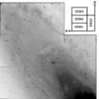
Figure 1: Reference image of the selected field of view in $V$ filter. The center of the field is at $\alpha=00^{\rm h}44^{\rm m}46^{\rm s}$ and $\delta=+41\degr 38\arcmin 20\arcsec$

The main part of the process is the determination of the convolution kernels. The kernels are constructed to match the reference image with each one of the remaining frames under study (supposedly with different seeing values). The DIA kernels are composed of Gaussian functions with constant widths and modified by polynomials. In our case, the kernels consist of three Gaussians with polynomials of orders 4, 3 and 2. A space-varying polynomial of order 4 has also been used to account for the spatial variation across the image. The resulting kernels are convolved with the reference image and subtracted from the original frames to obtain images containing only objects with brightness variations (plus noise).

The variability image is constructed from the differentiated images. This variability image contains all pixels considered to have light level variations. A pixel is considered to vary if it satisfies at least one of the following two conditions:

• There are more than 4 consecutive observations deviating more than 3$\sigma$ (where $\sigma$ is the standard deviation) from the base line flux in the same direction (brighter or fainter).

• There are more than 10 overall observations deviating more than 4$\sigma$ from the base line flux in the same direction.

The variability image is used to identify the variable stars. The reference image PSF is correlated with the variability image and all local maxima with correlation coefficients in excess of 0.7 are considered to be variable stars. Once the variable stars are located, PSF photometry is performed on all the differentiated images to obtain the differential fluxes. The differential fluxes can be transformed to the usual instrumental magnitudes through the following expression:

$$m_{i}=C-2.5\log(f_{0}+a\Delta f_{i})$$ (1)

where $\Delta f_{i}$ is the differential flux of a star in the $i$-th observation, $f_{0}$ is the base line flux on the reference image, $C$ is a zeropoint constant and $m_{i}$ is the instrumental magnitude of a star in the $i$-th observation.

The photometric package of DIA does not properly account for contamination from nearby stars in crowded fields (such as our case). Therefore, the $f_{0}$ values obtained with the DIA can potentially be severely overestimated. To obtain precise values for $f_{0}$, DAOPHOT PSF photometry (Stetson 1987) was applied to the reference image. Given that DIA and DAOPHOT photometry use different PSF definitions and functional forms, a scaling factor ($a$) is needed to transform the DIA fluxes into the DAOPHOT flux units (see Zebrun et al. 2001, for an extensive discussion). A synthetic image was created to compute the scaling factors. The synthetic image contains the representation of the DAOPHOT PSFs at the position of each variable star. The scaling factor at the position of each variable star was obtained from the comparison with the DIA photometry of each PSF. For similar PSFs, the scaling factor can be obtained with an error of 0.3% or less.

This process provided instrumental magnitudes for all the variable stars as well as all the stars in the reference image. Two main sources of potential systematic errors exist with this procedure, $f_{0}$ and $a$, but they affect the amplitudes of the light curves. However, as it is shown below in §5, the amplitudes of the fitted EBs are perfectly compatible with other results given in the literature.

3.3 Standard photometry

To transform instrumental to standard magnitudes, the observed Landolt (1992) standard stars were used. Although the standard stars were observed at different times during the night, the number of collected frames is not enough to accurately determine the atmospheric extinction. Therefore, as a first step, the M31 images obtained during the same night as the standard stars (30 images in total) were used to compute the coefficients needed to account for the atmospheric extinction. Aperture photometry of 20 bright, but not saturated, and isolated stars on the M31 frames was performed. For each night and filter, a linear fit, with dispersions ranging from 0.008 mag to 0.03 mag, was obtained.

As a second step, aperture photometry was performed on the standard stars. The instrumental magnitudes obtained were corrected with the atmospheric extinction coefficients. The resulting values were used to find the transformation coefficients between the instrumental magnitudes and the standard magnitudes. For each night and CCD the following relationship was determined:

$$v-V=A_{1}+A_{2}(B-V)$$ (2)

$$b-v=A_{3}+A_{4}(B-V)$$ (3)

where $b$ and $v$ are the instrumental magnitudes, $B$ and $V$ are the standard magnitudes and $A_{i}$ are the transformation coefficients. The resulting mean standard deviation of the fits is 0.02 mag.

The transformation coefficients cannot be directly applied to the M31 instrumental magnitudes because the latter are based on the reference image, which is a combination of different images. In addition, the transformation coefficients are determined from aperture photometry, while the M31 instrumental magnitudes have been determined from PSF photometry. For this reason, the only way to obtain standard magnitudes for the M31 stars is to apply the transformation coefficients to the frames obtained during the same nights as the standard stars.

PSF photometry is needed to find precise standard magnitudes of a reasonable number of objects in the M31 field since aperture photometry can only be applied to isolated stars. A sample of bright and isolated stars was employed to determine a scaling value used to transform the PSF magnitudes into aperture photometry values for each one of the 30 M31 frames. The scaling values and the transformation coefficients were used to obtain standard magnitudes for 18 426 objects in the field. A systematic difference was observed for the standard magnitudes obtained from the 2001 frames and, therefore, the obtained values were rejected. The standard magnitudes of every star in all the remaining frames (22 in total) were averaged and the standard deviation was considered a good estimation of its uncertainty.

The standard magnitudes resulting from this process were used to determine new transformation coefficients ($A_{i}$) for the reference images. Only 534 non-variable and non-saturated objects detected in all the frames and with an error below 0.04 mag were used for this purpose. This sample has good color and magnitude coverage, with $-0.3<B-V<1.7$ and $17.5<V<21.0$, providing fits with dispersions ranging from 0.013 mag to 0.019 mag, depending on the CCD. The obtained coefficients were applied to the reference images. The objects detected in the $V$ frame have been cross-matched with the objects detected in the $B$ frame. Only the objects identified within 0 $\aas@@fstack{\prime\prime}$33 (one pixel) have been included in the reference catalog, providing standard photometry for 236 238 objects. The error distributions, shown in Fig 2, have 37 241 objects with errors below 0.1 mag in both passbands. The limiting magnitudes of the photometric catalog are around $V\simeq 25.5$ and $B\simeq 26.0$, and it is estimated to be complete up to $V\simeq 22.3$ mag and $B\simeq 23.5$ mag. The same process was applied to transform the $m_{i}$ values in Eq. 1 to standard photometry in both $B$ and $V$ passbands for a total of 3 964 variable stars.

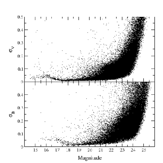
Figure 2: Error distribution for the entire photometric catalog containing 236 238 objects with photometry in both $V$ and $B$ passbands.

3.4 Astrometry

Standard coordinates for all detected objects were computed from several reference stars in the GSC 2.2.1. To ensure that the reference stars are uniformly distributed, each CCD was divided into 3$\times$6 sectors. Three reference stars (with $V\simeq 18$) were identified manually in each sector, yielding an initial list of 54 reference stars per CCD. Fits using third order linear equations with 2$\sigma$ scatter clipping were applied to determine the transformation of coordinates. After the iterative process at least two reference stars had to remain in each sector. Otherwise, an additional reference star was selected in the corresponding sector and the entire process was repeated.

The resulting coordinates have been compared with those in the GSC 2.2.1 catalog. A total of 724 objects with a position difference of less than $3\arcsec$ in the two catalogs were identified. As can be seen in Fig. 3, no systematics trends appear in the comparisons, which have dispersions of $\sigma_{\alpha}=0$ $\aas@@fstack{\prime\prime}$16 and $\sigma_{\delta}=0$ $\aas@@fstack{\prime\prime}$12.

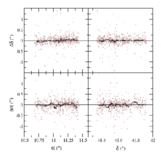
Figure 3: Differences between the coordinates obtained from our procedure and the coordinates from the GSC 2.2.1 catalog for 724 identified stars (circles). The line represents a running average.

3.5 Periodicity search

Since the observations were performed in five annual observing seasons, the data is very unevenly sampled. To overcome this major drawback for the determination of periodicities, a program based on the analysis of variance (Schwarzenberg-Czerny 1996) was used to compute the periodograms for each variable star and filter ($B$ and $V$). The periodograms were computed with 7 harmonics between 1 and 100 days because this setup was found to provide optimal results for the detection of EB systems, which constitute the main objective of the present survey. The lower limit in the period search is set from the consideration that EBs with periods below 1 day are likely to be foreground contact systems and therefore not of the interest of the survey. In addition, given the relatively long exposure time for each observation in the present survey (15 minutes), important brightness variations during the integration time could occur for the short period variables. These factors make the computational effort of extending the period search below 1 day not worthwhile. On the opposite end, the upper limit of 100 days was selected to detect as many long period Cepheids as possible.

For each variable star, two periodograms (one in $B$ and one in $V$) were used to obtain a consistent period determination. The resulting light curves were visually inspected to locate well-defined variability patterns, thus leading to the identification of a total of 437 EBs and 416 Cepheids. For several EBs and Cepheids, the period determination was a multiple of the true period and, therefore, it had to be recomputed.

For each variable star, the time of minimum of both light curves ($B$ and $V$) was used to compute a reference time. The time of minimum was computed from the Fourier series ($F^{\rm(7)}(t)$ in Schwarzenberg-Czerny 1996) that best fit each light curve.

4 The catalogs

4.1 Reference catalog

Photometry of the 236 238 objects detected in the reference images was grouped into the reference catalog. The reference catalog (Table 3) contains the object identifier, the right ascension, the declination, the $V$ standard magnitude in the reference image, the $V$ standard error, the $B$ standard magnitude in the reference image, the $B$ standard error and, in case that there is a previous identification, the corresponding identifier. The catalogs cross-matched with our reference catalog are GSC 2.2.1, DIRECT, LGGS (Massey et al. 2006) and Todd et al. (2005, hereafter T05). Photographic catalogs are identified in the previous works, specially in LGGS, and they are not cross-identified here.

According to the IAU recommendations, the identifier was built from the object position and taking into account the observational angular resolution. The resulting format is M31 JHHMMSSss+DDMMSSs. For the variable stars, the acronym was changed to M31V to indicate that they are also in the variable star catalog (see §4.2).

To show the general photometric properties of the obtained catalog, the color–magnitude diagram for the 37 241 objects with a photometric error below 0.1 mag in both $B$ and $V$ is shown in Fig. 4. From this diagram it can be seen that most of the stars in this catalog are stars at the top end of the main sequence, with some foreground giants and stars at the tip of the red giant branch.

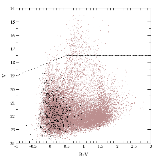
Figure 4: Color–magnitude diagram for 37 241 objects with photometric errors lower than 0.1 mag in both $B$ and $V$ in the reference catalog (grey dots) and 437 EBs (black circles). Stars above the dashed lines are saturated.

The obtained standard photometry depends on a number of zeropoint calibrations (§§3.2 and 3.3). Taking into account that an error in the standard magnitudes has a direct impact on the distance determination, it is extremely important to ensure that no systematic errors affect the photometry. For this reason, it is worthwhile to check the consistency of the standard magnitudes given here. Fortunately, there are two CCD surveys with $B$ and $V$ photometry of a large number of stars that overlap with the field under study: DIRECT (Macri 2004) and LGGS (Massey et al. 2006). The non-saturated objects of our survey ($V>17.5$ and $B>18.0$) were cross-identified with the magnitudes reported by the DIRECT group and by the LGGS group. For the DIRECT survey, a total of 14 717 and 7 499 objects were identified in $V$ and $B$ passbands, respectively (see Fig. 5). The comparison with the LGGS survey provided 36 353 common objects (see Fig. 6).

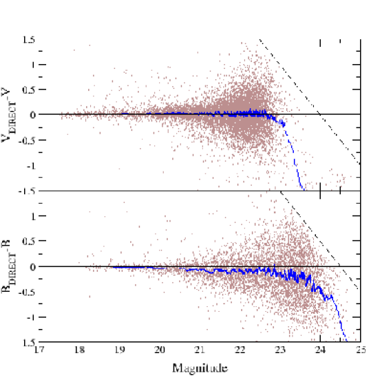
Figure 5: Differences with DIRECT standard magnitudes versus the magnitudes in the reference catalog. The comparison has 14 717 stars in $V$ and 7 499 in $B$. The dashed lines show the limiting magnitudes.

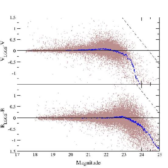
Figure 6: Differences with LGGS standard magnitudes versus the magnitudes in the reference catalog for a total amount of 36 353 stars in each passband. The dashed lines show the limiting magnitudes.

Although some trend is observed for the DIRECT $B$ magnitudes, the LGGS $B$ magnitudes are completely consistent with the magnitudes in our survey. Therefore, the $B$ standard magnitudes in the present paper are expected to have no systematic error. Regarding the $V$ magnitudes, some low-level systematics have been observed with the two catalogs. The DIRECT $V$ magnitudes are larger by about 0.02 mag than the values in the reference catalog, and the LGGS comparison shows an increasing trend towards larger magnitudes. The 5 768 objects with $V$ magnitudes in the three catalogs were used to study the observed systematics. The comparisons between the three catalogs always reveal some kind of trend and, therefore, it was impossible to conclude weather there are any (low-level) systematics affecting the $V$ standard magnitudes. In any case, the differences for the brightest stars ($V<20.5$ mag) are well below 0.03 mag. Taking into account that all the EBs than can be used for distance determination have $V<20.5$ (§5.2), this is the maximum systematic error that can exist in their $V$ standard magnitudes.

4.2 Variable star catalog

The 3 964 variable stars identified in the reduction process were grouped in the variable star catalog (Table 4). For each variable star, the corresponding identifier (see §4.1), the right ascension, the declination, the intensity–averaged $V$ magnitude (Eq. $(9)$ in Saha & Hoessel 1990), the mean $V$ error, the intensity–averaged $B$ magnitude, the mean $B$ error, the number of observations in $V$, the number of observations in $B$, the reference time (in HJD), the period (in days) and a label, indicating weather the variable star was identified as an EB or a Cepheid, are provided.

Although a period estimate is given for each variable star, obviously not all the variable stars are periodic. When comparing the window function with the period distribution for all variable stars (see Fig. 7), it is clear that many of the period determinations are just an alias introduced by the window function, specially for those over five days. Therefore, a significant number of the variable stars are, in fact, non-periodic variables or variables with a period out of the studied range (1–100 days). All light curves (time series photometry) are also provided (Table 5) together with the variable star catalog. For each variable star and observation, the observed time (in JD), the standard magnitude ($V$ or $B$) and the standard error are given.

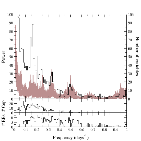
Figure 7: Top: Window function for the studied period range (lines) and frequency distribution for all the stars in the variable star catalog (histogram). Middle: Frequency distribution for the Cepheids in the variable star catalog. Bottom: Frequency distribution for the eclipsing binaries in the variable star catalog.

5 Eclipsing binaries

5.1 Complete sample

The color–magnitude diagram (see Fig. 4) reveals that most of the detected EB systems contain high-mass components belonging to the top of the main sequence. Taking into account that most of the systems have periods shorter than 10 days (and all of them have periods shorter than 30 days), a large fraction of EB systems are non-detached systems.

Part of the images in the present survey were also reduced by T05 and reported the detection of 127 EB systems. Of those, 123 stars have been detected in our reference catalog, 92 are in the variable star catalog and 90 have also been classified as EBs. The maximum $V^{\rm max}$ and $B^{\rm max}$ values for the 90 systems identified were matched with the magnitudes presented in T05 (see Fig. 8). A clear systematic trend can be observed in the $V$ filter. In addition, Fig. 8 also reveals that the $B^{\rm max}_{\textrm{\scriptsize\cite[citealias]{\@@bibref{Phrase1}{A2005015}{\@@citephrase{T05}}{}}}}$ magnitudes are lower than our $B^{\rm max}$ values.

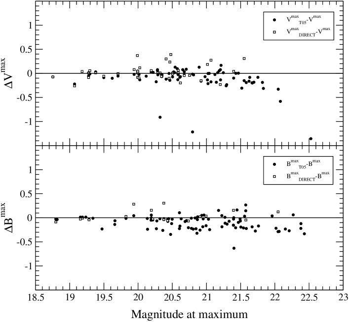
Figure 8: Differences between the DIRECT maximum magnitudes (open squares), the T05 maximum magnitudes (filled circles) and the maximum magnitudes for all the crossed EBs of the variable star catalog.

When inspecting the origin of such discrepancy, we observed that all the EBs labeled f2BEB and f3BEB in T05 had lower magnitude values than the EBs in our variable star catalog. Since 14 of these EBs have also DIRECT $V^{\rm max}$ magnitudes, and 5 of them have DIRECT $B^{\rm max}$ values (Kaluzny et al. 1998; Stanek et al. 1998, 1999; Bonanos et al. 2003), the mean differences were computed (Table 6). Although the number of cross-matched EBs is small, their mean differences seem to indicate that the magnitudes reported in T05 for the f2BEB and f3BEB EBs suffer from a systematic offset. On the other hand, the magnitude values for the remaining EBs (f1BEB and f4BEB) are fairly compatible in the three catalogs.

Table 6: Mean differences for the magnitudes at maximum of the EBs labeled f2BEB and f3BEB in T05.

Comparison	Differences
$V^{\rm max}_{\textrm{\scriptsize DIRECT}}-V^{\rm max}$	0.062$\pm$	0.047
$V^{\rm max}_{\textrm{\scriptsize\cite[citealias]{\@@bibref{Phrase1}{A2005015}{\@@citephrase{T05}}{}}}}-V^{\rm max}$	-0.104$\pm$	0.015
$V^{\rm max}_{\textrm{\scriptsize\cite[citealias]{\@@bibref{Phrase1}{A2005015}{\@@citephrase{T05}}{}}}}-V^{\rm max}_{\textrm{\scriptsize DIRECT}}$	-0.166$\pm$	0.057
$B^{\rm max}_{\textrm{\scriptsize DIRECT}}-B^{\rm max}$	0.054$\pm$	0.039
$B^{\rm max}_{\textrm{\scriptsize\cite[citealias]{\@@bibref{Phrase1}{A2005015}{\@@citephrase{T05}}{}}}}-B^{\rm max}$	-0.214$\pm$	0.026
$B^{\rm max}_{\textrm{\scriptsize\cite[citealias]{\@@bibref{Phrase1}{A2005015}{\@@citephrase{T05}}{}}}}-B^{\rm max}_{\textrm{\scriptsize DIRECT}}$	-0.268$\pm$	0.046

5.2 Light curve fitting

From all the variable stars identified as EBs only those systems with a precise determination of their fundamental properties can be used as distance determination targets. Taking into account that medium–resolution spectra are needed to obtain precise fundamental properties, and considering the fact that the largest currently available facilities are the 8–10 m class telescopes, only the brightest EB systems (with $V^{\rm mean}<20.5$) were selected for further study. In addition, the most precise fundamental properties can be achieved only for those systems with deep eclipses, and thus we further selected only those EBs with $\Delta B\geq 0.2$ mag and $\Delta V\geq 0.2$ mag.

The criteria above provided a list of 29 systems from the initial sample of 437 EBs. Of these, 5 systems were rejected because of the large scatter in their light curves (probably from the contamination of a brighter nearby star), leaving a total amount of 24 EBs selected for detailed further analysis. The particular properties of each EB can have an important influence on the precise determination of its fundamental parameters. To obtain the best distance determination targets, a preliminary fit was performed, with the 2003 version of the Wilson & Devinney (1971) program (W-D), to the selected sample of 24 EBs.

The fitting process was carried out, in an iterative manner, by considering both light curves ($B$ and $V$) simultaneously. For those systems previously identified by the DIRECT group their $V$ light curve was also included in the fitting process. This provided an additional check on the consistency of the resulting photometry, because the DIRECT photometry was calculated from a PSF rather than using a DIA algorithm. Once a converging solution was achieved, a $4\sigma$ clipping was performed on all the light curves to eliminate (normally a few) outlier observations.

A certain configuration has to be assumed for each solution of W-D. Two basic configurations were considered for each EB system: detached and semi-detached. Generally, the final fit in each one of the configurations provided some clues about the real configuration of the EB system. However, all systems showing non-zero eccentricity (secondary eclipse phase not exactly at 0.5) were considered to be detached EB systems. In some specific cases, a sinusoidal $O-C$ was observed when studying the fit residuals, with one quadrature being brighter than the other. This is known as the O’Connell effect. In the case of interacting high-mass systems, such effect can be explained by the presence of an equatorial hot spot on the surface of one the components. Such hot spot is supposed to the consequence of impacting material arising from mass transfer between the components in a Roche-lobe filling configuration (semi-detached). The exact parameters of the spot cannot be obtained from the available data (strong degeneracies exist; Fitzpatrick et al. 2003) and, therefore, the spot parameters presented here are not necessarily physically valid but only capable of providing a good fit to the variations in the light curves.

Each EB is a particular case and careful selection of the adjustable parameters was performed individually. In general, the parameters fitted with W-D are: the time of minimum ($t_{\rm min}$), the period ($P$), the inclination ($i$), the effective temperature of the secondary ($T^{\rm eff}_{2}$), the normalized potential of primary ($\Omega_{1}$), the normalized potential of secondary ($\Omega_{2}$), for detached systems only, and the luminosity of the primary ($L_{1}$). For the eccentric systems, in addition, the eccentricity ($e$) and the argument of the periastron ($\omega$) were also fitted. In some cases of semi-detached systems, the mass ratio ($q$) was treated as a free parameter. Finally, a third light ($l_{3}$) contribution was included for the final solutions of the EB systems. Taking into account that the field under study is extremely crowded, it is not surprising that some EBs may have a significant third light contribution (see §5.3 for a more extended discussion on this topic). In addition, the obtained values of the third light contribution provide a first check on the realistic determination of the fundamental properties and give an indication that the scaling factor determinations ($a$ in Eq. 2) are correct. Indeed, an error in the scaling factor has exactly the same effect as a third light contribution. The limb-darkening coefficients (square-root law) were computed at each iteration from Kurucz ATLAS9 atmosphere models and the gravity brightening coefficients, as well as the bolometric albedos, were fixed to unity (assuming components with radiative envelopes).

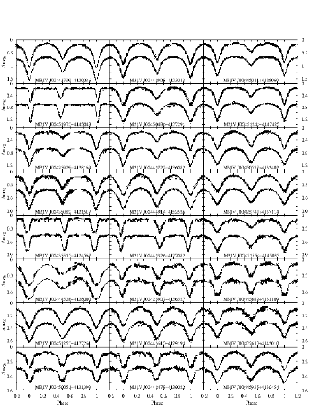
Figure 9: $B$ (up) and $V$ (down) light curves for the 24 fitted EBs. The corresponding Wilson–Devinney fits are also plotted (lines).

Note that most of the solutions have a large number of free parameters. To some extent, the values presented here rely on the adoption of the mass ratio and, therefore, the fit results (in Table 7 and Fig. 9) should be regarded as preliminary until radial velocity curves are obtained. For some of the binaries the values given in Table 7 need additional comments:

• M31V J00444528+4128000. This is the brightest EB system detected. A converging fit could not be achieved because of variations of the light curve at the second quadrature. The reason is so far unidentified but it could be due to a varying hot spot, an accretion disk or intrinsic variability of a supergiant component. This makes the system an interesting target for future follow-up observations.

• M31V J00442326+4127082. The DIRECT light curve reveals a variation in the argument of periastron thus indicating the presence of rapid apsidal motion (1.9$\pm$0.6 deg year^-1). Even taking into account the important third light contribution, the radial velocity curves can provide valuable information to study the real nature of this detached, eccentric system.

• M31V J00443799+4129236. Radial velocity curves have already been acquired with the 8-m Gemini North telescope and more accurate fundamental parameters have been derived, in Paper I, from the fit of both radial velocity and light curves, as well as from the fit of the atmospheric parameters from the spectra. However, we decided to consider this system within the current homogeneous analysis and thus the comparison of the parameters presented here and those in Paper I provides an idea of the accuracy of the parameters in semi-detached systems when the mass ratio is unknown.

• M31V J00451973+4145048. A likely large error in the scaling factor causes a large negative $V$ third light contribution. In any case, a correct third light contribution is obtained in the DIRECT light curve and, therefore, the fundamental parameters are expected to be correctly determined.

• M31V J00444914+4152526. An equatorial hot spot was assumed for this EB system. The best fit yields a spot with a temperature ratio of 1.2, at a longitude of $246\pm 14$ deg and a size of $17\pm 3$ deg.

• M31V J00442478+4139022. The large scatter of the DIRECT $V$ light curve prevented a reliable fit from being achieved. Consequently, the DIRECT light curve was not used.

• M31V J00445935+4130454. A very slight O’Connell effect was observed in this EB system, suggesting the presence of a hot spot. The best fit, with a temperature ratio of 1.1, yields a spot at $280\pm 60$ deg and a size of $21\pm 11$ deg.

The obtained values provide a good estimation of the potential of each EB system to become a good distance determination target. In general, the best distance determination targets should have low third light contribution and a luminosity ratio close to unity. On one hand, an important third light contribution would lead to an underestimation of the observed standard magnitudes for the EB system. Although the third light can be modelled, the resulting values may have uncertainties that are large enough to have a sizeable negative effect on the accuracy of the distance determination. On the other hand, EBs with luminosity ratios close to unity will have spectra with visible lines for the two components, thus making possible the determination of accurate fundamental properties. Taking into account the obtained values, several EBs have already been selected as targets to obtain radial velocity measures and, in fact, already one of them has been used to determine the first direct distance to M31 (Paper I).

5.3 Blending

Special care has to be taken with the magnitudes reported in the present paper. As mentioned above, the FWHM of the reference images is around $1\arcsec$. At the distance of M31 ($\sim$770 kpc, Paper I, ) this corresponds to more than 3.5 pc. Therefore, it is highly probable that a large fraction of the identified objects in the reference catalog are, in fact, a blend of several stars. In addition, the blending effect can significantly modify the observed amplitudes of variable stars and therefore their derived mean magnitudes can also be in error. Mochejska et al. (2000) studied this problem for Cepheid variables in M31 and arrived at the conclusion that blending affect the $V$ Cepheid flux at the 19% level.

It has been noted before (T05) that such blending would seriously hamper the accurate determination of fundamental properties and distances of M31 EBs. While this is true for Cepheid variables, EB systems are a particular case of variable stars in which their variations obey a well-defined physical model. Therefore, blending effects are easily and seamlessly incorporated in the EB modelling as an additional (third) light contribution. While special care has to be taken (e.g., check for physical consistency between the third light values for different passbands), the presence of a third light does not preclude the determination of reliable properties for the components. In any case, no systematic errors in the distances of EBs will arise from blending because the analysis can detect its effects in a natural manner. Note that the mean $V$ third light value for the 24 fitted systems in our analysis is of 10% and it would be around 20% from a rough scaling to single stars. This is in excellent agreement with the value derived by Mochejska et al. (2000).

6 Conclusions

Deep and high-quality time-series photometry has been obtained for a region in the North–Eastern quadrant of M31. The present survey is the deepest photometric survey so far obtained in M31. The photometry has been checked for compatibility with that from other surveys and, therefore, our resulting catalog can be used as a reference to extend the time baseline of future stellar surveys in M31.

The study of the variable star population has revealed about 4 000 variables. Further analysis is needed for most of them for a proper classification but over 800 variable stars have already been identified as EBs and Cepheids. The study of the Cepheid variables will be the subject of a forthcoming publication (Vilardell et al. 2006). In the current paper we have presented the analysis of the EB population, which has resulted in an extensive list of EBs suitable for accurate determinations of the components’ physical properties and their distances. The catalog provided here constitutes an excellent masterlist to select systems for further analysis. For example, the resulting physical properties will be an important tool to study stellar evolution of massive stars in another galaxy and, therefore, in a completely independent chemical environment. But, in accordance with the main goal of the the present survey, the technique of determining accurate distances from EBs has been demonstrated in Paper I to harbor great potential. Full analysis of an additional 5–10 EBs from the sample provided here can result in a distance determination to M31 with a relative uncertainty of 2–3% and free from most systematic errors. This will represent the most accurate and reliable distance determination to this important Local Group galaxy.

Table 7: Fundamental properties of the 24 EBs with Wilson–Devinney fits (see text for nomenclature).

Identifier	Conf.a	$V^{\rm max}$	P		$i$		$e$		$\omega$		$R_{1}/a^{b}$		$R_{2}/a^{b}$
$[$M31V $]$		[mag]	[days]		[deg]				[deg]
J00444528+4128000	SD	18.854	11.543654$\pm$	0.000211	78.0$\pm$	1.3	0.0		–		0.556$\pm$	0.009	0.277$\pm$	0.002
J00435515+4124567	D	19.164	6.816191$\pm$	0.000067	89.1$\pm$	4.4	0.105$\pm$	0.010	327.4$\pm$	7.8	0.160$\pm$	0.007	0.281$\pm$	0.012
J00442326+4127082	D	19.242	5.752689$\pm$	0.000037	87.3$\pm$	2.4	0.189$\pm$	0.019	51.3$\pm$	4.7	0.215$\pm$	0.017	0.267$\pm$	0.025
J00451253+4137261	SD	19.366	2.358359$\pm$	0.000010	75.4$\pm$	3.0	0.0		–		0.369$\pm$	0.023	0.372$\pm$	0.007
J00443799+4129236	SD	19.428	3.549696$\pm$	0.000012	83.3$\pm$	0.6	0.0		–		0.330$\pm$	0.019	0.390$\pm$	0.006
J00442928+4123013	SD	19.475	3.168969$\pm$	0.000006	86.4$\pm$	2.5	0.0		–		0.329$\pm$	0.014	0.403$\pm$	0.005
J00450486+4137291	SD	19.536	3.094681$\pm$	0.000013	75.7$\pm$	3.0	0.0		–		0.316$\pm$	0.021	0.390$\pm$	0.008
J00451973+4145048	D	19.572	8.130670$\pm$	0.000087	87.2$\pm$	2.4	0.252$\pm$	0.027	109.1$\pm$	1.8	0.216$\pm$	0.014	0.149$\pm$	0.012
J00450051+4131393	D	19.756	5.211976$\pm$	0.000044	81.7$\pm$	1.2	0.040$\pm$	0.015	120.0$\pm$	14.1	0.128$\pm$	0.005	0.349$\pm$	0.011
J00444914+4152526	SD	19.772	2.626992$\pm$	0.000010	72.5$\pm$	1.5	0.0		–		0.340$\pm$	0.015	0.384$\pm$	0.005
J00442478+4139022	D	20.034	4.762310$\pm$	0.000068	79.9$\pm$	1.2	0.027$\pm$	0.008	188.8$\pm$	33.4	0.105$\pm$	0.003	0.333$\pm$	0.014
J00443610+4129194	SD	20.038	2.048644$\pm$	0.000006	70.6$\pm$	1.7	0.0		–		0.290$\pm$	0.018	0.369$\pm$	0.007
J00425907+4136527	D	20.060	5.874724$\pm$	0.000069	81.0$\pm$	1.1	0.163$\pm$	0.016	70.8$\pm$	2.2	0.344$\pm$	0.013	0.157$\pm$	0.011
J00452554+4145035	SD	20.090	5.009412$\pm$	0.000047	82.3$\pm$	3.4	0.0		–		0.247$\pm$	0.020	0.393$\pm$	0.008
J00442722+4136082	SD	20.098	4.518795$\pm$	0.000016	86.1$\pm$	1.7	0.0		–		0.308$\pm$	0.018	0.344$\pm$	0.009
J00453244+4147425	SD	20.141	2.787856$\pm$	0.000010	78.4$\pm$	1.7	0.0		–		0.238$\pm$	0.012	0.342$\pm$	0.007
J00445935+4130454	SD	20.166	2.668419$\pm$	0.000023	68.1$\pm$	1.9	0.0		–		0.277$\pm$	0.025	0.347$\pm$	0.013
J00450537+4133402	SD	20.326	1.769903$\pm$	0.000005	75.4$\pm$	2.5	0.0		–		0.351$\pm$	0.025	0.350$\pm$	0.010
J00432610+4142010	SD	20.340	4.274429$\pm$	0.000065	75.9$\pm$	3.6	0.0		–		0.206$\pm$	0.027	0.413$\pm$	0.014
J00445682+4131109	D	20.360	4.207679$\pm$	0.000036	87.2$\pm$	4.5	0.0		–		0.345$\pm$	0.015	0.158$\pm$	0.015
J00435082+4121517	D	20.367	2.176672$\pm$	0.000011	79.6$\pm$	4.1	0.0		–		0.305$\pm$	0.026	0.358$\pm$	0.031
J00425743+4137114	SD	20.388	1.916302$\pm$	0.000008	73.9$\pm$	2.9	0.0		–		0.364$\pm$	0.019	0.379$\pm$	0.006
J00425929+4138169	D	20.450	5.591515$\pm$	0.000045	85.5$\pm$	4.0	0.0		–		0.340$\pm$	0.011	0.264$\pm$	0.016
J00445011+4128069	D	20.456	2.861046$\pm$	0.000009	80.2$\pm$	2.4	0.0		–		0.347$\pm$	0.013	0.286$\pm$	0.013

^aConfiguration. (D): Detached, (SD): Semi–detached.

${}^{b}R_{1}/a$ and $R_{2}/a$ are the relative radii of the components, where $a$ is the semi-major axis of the system.

Identifier	$T_{2}^{\rm eff}/T_{1}^{\rm eff}$		$(L_{2}/L_{1})^{B}$		$(L_{2}/L_{1})^{V}$		$(L_{2}/L_{1})^{D}$		$l_{3}^{B}$		$l_{3}^{V}$		$l_{3}^{D}$
$[$M31V $]$
J00444528+4128000	0.453$\pm$	0.033	0.0513$\pm$	0.0003	0.0575$\pm$	0.0004	0.0575$\pm$	0.0004	0.0		0.0		0.0
J00435515+4124567	0.911$\pm$	0.018	2.69$\pm$	0.09	2.70$\pm$	0.08	–		0.055$\pm$	0.032	$-$0.005$\pm$	0.030	–
J00442326+4127082	0.890$\pm$	0.027	1.25$\pm$	0.13	1.27$\pm$	0.14	1.27$\pm$	0.15	0.329$\pm$	0.039	0.336$\pm$	0.043	0.328$\pm$	0.051
J00451253+4137261	0.885$\pm$	0.020	0.80$\pm$	0.08	0.82$\pm$	0.09	0.82$\pm$	0.12	0.285$\pm$	0.056	0.308$\pm$	0.059	0.325$\pm$	0.070
J00443799+4129236	0.772$\pm$	0.012	0.88$\pm$	0.04	0.90$\pm$	0.04	0.90$\pm$	0.04	0.0		0.0		0.0
J00442928+4123013	0.857$\pm$	0.011	1.17$\pm$	0.05	1.19$\pm$	0.05	1.19$\pm$	0.06	0.042$\pm$	0.035	0.027$\pm$	0.032	0.022$\pm$	0.034
J00450486+4137291	0.787$\pm$	0.015	1.01$\pm$	0.12	1.03$\pm$	0.12	1.03$\pm$	0.13	0.016$\pm$	0.098	$-$0.041$\pm$	0.093	$-$0.033$\pm$	0.096
J00451973+4145048	0.894$\pm$	0.016	0.34$\pm$	0.06	0.35$\pm$	0.06	0.34$\pm$	0.07	0.041$\pm$	0.077	$-$0.136$\pm$	0.096	0.115$\pm$	0.096
J00450051+4131393	0.993$\pm$	0.005	7.67$\pm$	0.35	7.74$\pm$	0.38	7.73$\pm$	1.47	0.063$\pm$	0.025	0.069$\pm$	0.024	0.055$\pm$	0.086
J00444914+4152526	0.957$\pm$	0.026	1.20$\pm$	0.09	1.21$\pm$	0.09	–		0.003$\pm$	0.046	0.009$\pm$	0.047	–
J00442478+4139022	0.848$\pm$	0.004	7.48$\pm$	0.34	7.65$\pm$	0.35	–		0.0		0.0		–
J00443610+4129194	0.946$\pm$	0.020	1.51$\pm$	0.18	1.52$\pm$	0.18	1.52$\pm$	0.22	0.067$\pm$	0.034	0.051$\pm$	0.032	0.016$\pm$	0.047
J00425907+4136527	1.046$\pm$	0.021	0.22$\pm$	0.02	0.22$\pm$	0.02	0.22$\pm$	0.02	0.053$\pm$	0.017	0.051$\pm$	0.029	0.034$\pm$	0.023
J00452554+4145035	0.810$\pm$	0.018	1.72$\pm$	0.13	1.78$\pm$	0.13	1.78$\pm$	0.27	0.169$\pm$	0.014	0.162$\pm$	0.023	0.227$\pm$	0.029
J00442722+4136082	0.747$\pm$	0.008	0.72$\pm$	0.05	0.76$\pm$	0.05	0.76$\pm$	0.06	0.109$\pm$	0.009	0.130$\pm$	0.010	0.119$\pm$	0.014
J00453244+4147425	0.728$\pm$	0.009	1.14$\pm$	0.11	1.20$\pm$	0.12	1.20$\pm$	0.17	0.036$\pm$	0.022	0.018$\pm$	0.026	0.093$\pm$	0.090
J00445935+4130454	0.857$\pm$	0.063	1.22$\pm$	0.24	1.25$\pm$	0.25	–		0.169$\pm$	0.079	0.219$\pm$	0.082	–
J00450537+4133402	0.940$\pm$	0.015	0.88$\pm$	0.10	0.89$\pm$	0.10	0.89$\pm$	0.13	$-$0.055$\pm$	0.110	$-$0.027$\pm$	0.102	$-$0.037$\pm$	0.117
J00432610+4142010	0.838$\pm$	0.028	3.15$\pm$	0.77	3.23$\pm$	0.79	–		0.243$\pm$	0.043	0.309$\pm$	0.061	–
J00445682+4131109	0.891$\pm$	0.024	0.18$\pm$	0.03	0.18$\pm$	0.03	0.18$\pm$	0.04	0.118$\pm$	0.076	0.129$\pm$	0.087	0.153$\pm$	0.117
J00435082+4121517	0.789$\pm$	0.019	0.89$\pm$	0.18	0.93$\pm$	0.19	–		0.245$\pm$	0.074	0.211$\pm$	0.091	–
J00425743+4137114	0.921$\pm$	0.014	0.94$\pm$	0.11	0.96$\pm$	0.11	–		0.165$\pm$	0.063	0.219$\pm$	0.070	–
J00425929+4138169	0.548$\pm$	0.011	0.17$\pm$	0.02	0.19$\pm$	0.02	0.19$\pm$	0.02	0.195$\pm$	0.042	0.203$\pm$	0.049	0.139$\pm$	0.045
J00445011+4128069	0.603$\pm$	0.016	0.25$\pm$	0.03	0.26$\pm$	0.03	0.26$\pm$	0.04	$-$0.012$\pm$	0.090	$-$0.004$\pm$	0.080	0.001$\pm$	0.105