Probing Primordial Magnetic Fields with the 21cm Fluctuations

Abstract

Primordial magnetic fields possibly generated in the very early universe are one of the candidates for the origin of magnetic fields observed in many galaxies and galaxy clusters. After recombination, the dissipation process of the primordial magnetic fields increases the baryon temperature. The Lorentz force acts on the residual ions and electrons to generate density fluctuations. These effects are imprinted on the cosmic microwave background (CMB) brightness temperature fluctuations produced by the neutral hydrogen 21cm line. We calculate the angular power spectrum of brightness temperature fluctuations for the model with the primordial magnetic fields of a several nano Gauss strength and a power-law spectrum. It is found that the overall amplitude and the shape of the brightness temperature fluctuations depend on the strength and the spectral index of the primordial magnetic fields. Therefore, it is expected that the observations of the CMB brightness temperature fluctuations give us a strong constraint on the primordial magnetic fields.

1 introduction

Observations reveal existence of magnetic fields on very large scale, i.e., galaxies and clusters of galaxies. It is found that these magnetic fields typically have a few $\mu$Gauss strengths and relatively large coherent scales, i.e., a few tens of kpc for clusters of galaxies and a few kpc for galaxies (Kronberg, 1994). The origin of such magnetic fields has not yet known while many ideas have been proposed. Perhaps it may be one of the most important remaining problems of cosmology and astrophysics to find out the origin and evolution of magnetic fields in the history of the universe.

The most conventional idea is that such magnetic fields were formed due to the astrophysical processes such as Biermann battery (Biermann, 1950) in stars and supernova explosions. Then these seed magnetic fields were amplified by the dynamo process. Eventually, supernova winds or active galactic nuclei (AGN) jets may spread these magnetic fields into inter-galactic medium (for a comprehensive review see Widrow 2002). However, it is still little known about the efficiency of the dynamo process in the expanding universe. It is particularly difficult for the astrophysical processes to explain observed magnetic fields with very large coherent scales in galaxy clusters (Kim et al., 1990; Kim et al., 1991). A recent observation suggests existence of magnetic fields in high redshift galaxies (Kronberg et al., 1992). These galaxies may be dynamically too young for the dynamo process to play a role.

An alternative scenario is that magnetic fields were formed in the very early universe. Many authors have suggested various generation mechanisms of the primordial magnetic fields in the early universe. One can introduce an exotic coupling between electro-magnetic and scalar fields to generate magnetic fields during the inflation epoch. Or one can consider bubble collisions during cosmological phase transitions such as QCD or electroweak for generation of magnetic fields. For a detailed review, see Giovannini (2004). In this alternative scenario, one may directly obtain the nano Gauss primordial magnetic fields which are sufficient enough to explain $\mu$Gauss magnetic fields observed at present since the adiabatic compression due to the structure formation could easily amplify the primordial magnetic fields by a factor $\sim 10^{3}$. In this case, there is no need of the dynamo process. However, if the seed magnetic fields generated in the early universe were too weak, the dynamo process is required even in this scenario while the coherent length could be very large unlike the astrophysical processes.

If the magnetic fields were generated in the very early universe, such primordial magnetic fields may play an important role for various cosmological phenomena. There are many previous works to constrain the strength of the primordial magnetic fields from Big Bang Nucleosynthesis (BBN), temperature anisotropies and polarization of Cosmic Microwave Background (CMB), or structure formation. These constraints give us clues to the origin of large-scale magnetic fields, and when and how magnetic fields were generated.

The primordial magnetic fields affect on BBN through the enhancement of the cosmological expansion rate as neutrinos or the modification of the reaction rates of the light elements. The limit on the magnetic field strength from BBN is $B_{0}\la 7\times 10^{-5}$Gauss where $B_{0}$ is the comoving magnetic field strength (Cheng et al., 1996; Kernan et al., 1996).

The black-body energy spectrum of CMB could be distorted by the primordial magnetic fields through the dissipation process. The severe constraint on the spectrum distortion from COBE/FIRAS observation leads to $B_{0}\la 3\times 10^{-8}$Gauss on comoving scales of $400$–$600$pc at redshift $z\ga 2\times 10^{6}$ (Jedamzik et al., 2000).

The primordial magnetic fields produce CMB temperature anisotropies on various scales. On very large scales, coherent magnetic fields generate the anisotropic expansion of the universe. Magnetic fields with the present-horizon-size coherent scale are constrained as $B_{0}\la 10^{-9}$Gauss (Barrow et al., 1997). On intermediate or small scales, magnetic pressure modifies the acoustic oscillations of baryon-photon fluids. Or Alfven mode (fluid vorticity) induces temperature anisotropies. Constraints on the primordial magnetic fields with $100$Mpc–$1$Mpc coherent scales from WMAP and other CMB experiments are $B_{0}\la 10^{-8}$Gauss (Adams et al., 1996; Mack et al., 2002; Lewis, 2004; Yamazaki et al., 2005; Tashiro et al., 2005). Moreover CMB polarization suffers from magnetic fields. The Faraday rotation of the polarization is caused when CMB crosses the ionized inter-galactic medium (IGM) if there exist magnetic fields (Scóccola et al., 2004; Kosowsky et al., 2005). The fluid vorticity induced by magnetic fields can generate B-mode (parity odd) polarization as well as E-mode (parity even) (Subramanian et al., 2003; Tashiro et al., 2005). We expect to have much stringent limits on the primordial magnetic fields by future CMB observations, e.g., Planck (http://www.rssd.esa.int/Planck).

The primordial magnetic fields may play an important role for the structure formation in the universe. The Lorentz force of the primordial magnetic fields could induce density fluctuations once the universe becomes transparent after recombination (Wasserman, 1978; Kim et al., 1996; Subramanian & Barrow, 1998; Gopal & Sethi, 2003). The magnetic tension and pressure are more effective on small scales where the entanglements of magnetic fields are larger. Therefore, if there exist the primordial magnetic fields, it is expected that there is the additional power in the density power spectrum on small scales and these power induces the early structure formation (Sethi & Subramanian, 2005; Tashiro & Sugiyama, 2006).

Thermal evolution of baryons after decoupling from photons, redshift $z\sim 200$, could be also modified by the existence of the primordial magnetic fields (Sethi & Subramanian, 2005) since the dissipation of the primordial magnetic fields work as the heat source. The dissipation mechanisms are the ambipolar diffusion and the direct cascade decay of magnetic fields.

Both the structure formation and the thermal evolution of baryons are closely connected to reionization of IGM. Hence, we can suspect that the reionization process can be strongly affected by the existence of the primordial magnetic fields.

One of the best probes of the reionization process of IGM is the CMB brightness temperature fluctuations induced by neutral hydrogens through the 21cm line. In this paper, therefore, we examine the effect of the primordial magnetic fields on the CMB brightness temperature fluctuations produced by the redshifted hydrogen 21cm line. The hydrogen 21cm line is caused by a spin flip of the electron in a neutral hydrogen atom. The neutral hydrogen atoms produce the brightness temperature fluctuation of CMB by 21cm line absorption from and emission into CMB. The amplitude of the brightness temperature fluctuations depends on the hydrogen density, ionization fraction of hydrogens and hydrogen temperature. Therefore observations of the brightness temperature fluctuations at wave length $21(1+z)$cm reveal the density fluctuations and the ionization process at redshift $z$ (Loeb & Zaldarriaga, 2004; Bharadwaj & Ali, 2004; Cooray, 2005; Ali et al., 2005). Recent efforts to measure redshifted 21cm line such as LOFAR (http://www.lofar.org), MWA (http://web.haystack.mit.edu/arrays/MWA/MWA.html) and SKA (http://www.skatelescope.org), will soon give us clues of dark ages of the universe.

This paper is organized as follows. In Sec. II, we discuss the effect of the primordial magnetic fields on the hydrogen temperature and the density fluctuations. In Sec. III, we summarize CMB bright temperature fluctuations produced by the hydrogen 21cm line. In Sec. IV, we compute the angular power spectrum of bright temperature fluctuations with the primordial magnetic fields and discuss the effect of the primordial magnetic fields. Sec. V is devoted to summary. Throughout the paper, we take WMAP values for the cosmological parameters, i.e., $h=0.71\ (H_{0}=h\times 100{\rm Km/s\cdot Mpc})$, $T_{0}=2.725$K, $h^{2}\Omega_{\rm b}=0.0224$ and $h^{2}\Omega_{\rm m}=0.135$ (Spergel et al., 2003). And $\hbar$ and $c$ are Planck’s constant over $2\pi$ and speed of light, respectively.

2 Effects of the primordial magnetic fields on thermal history and structure formation

After recombination, the primordial magnetic fields affect the thermal history and the structure formation of the universe. In this section we summarize how the existence of magnetic fields modifies them.

Let us discuss the evolution of the primordial magnetic fields and the resultant power spectrum. First, we postulate that the primordial magnetic field lines are frozen-in to baryon fluid in the early universe. This assumption leads to the time evolution as

$${\bf B}_{0}({\rm x})=a^{2}(t){\bf B}(t,{\rm x}),$$ (1)

where $a(t)$ is the scale factor, which is normalized to the present value, and ${\bf B}_{0}$ is the comoving strength of magnetic fields. Since the baryon fluid is highly conductive through the entire history of the universe, this relation can be hold as far as magnetic fields do not suffer from non-linear processes such as direct cascade induced by turbulent motion of eddies.

Next, we assume that the primordial magnetic fields are isotropic and homogeneous Gaussian random fields, and have a power-law spectrum as

$$\langle B_{0i}({\bf k_{1}})B_{0j}^{*}({\bf k_{2}})\rangle={(2\pi)^{3}\over 2}\delta({\bf k_{1}-k_{2}})\left(\delta_{ij}-{k_{1i}k_{2i}\over k_{1}^{2}}\right)B^{2}_{0}(k),$$ (2)

$$4\pi k^{3}B^{2}_{0}(k)=(n+3)\left({k\over k_{\rm c}}\right)^{n+3}B_{\rm c}^{2}\qquad{\rm for}\ (k<k_{\rm c}),$$ (3)

where $k_{\rm c}$ is the cutoff wave-number and $n$ is the spectral index. Here $B_{\rm c}$ is the root-mean-square amplitude of the magnetic field strength in real space.

The cutoff in the power spectrum appears due to dissipation of magnetic fields associated with the nonlinear direct cascade process (Jedamzik et al., 1998; Subramanian & Barrow, 1998; Banerjee & Jedamzik, 2004). The direct cascade process transports the magnetic field energy from large scales to small scales through the breaking of flow eddies and generates the peak in the energy spectrum resultantly. The time-scale of the eddy breaking at the scale $l$ is $l/v$, where $v$ is the baryon fluid velocity. The direct cascade occurs when the eddy breaking time-scale is equal to the Hubble time $H^{-1}$. Once the direct cascade takes place, the “red” power-law tail is produced in the power spectrum of magnetic fields. In order to simplify following calculations, however, we assume that the direct cascade process produces a sharp cutoff instead of the power-law cutoff in the spectrum.

Once the universe becomes transparent after recombination, baryons decouple from photons and their velocity starts to increase. Eventually the velocity achieves the value determined by the equipartition between the magnetic field energy and the kinetic energy of the baryon fluid, namely the Alfven velocity, $v_{\rm A}\equiv cB_{0}/\sqrt{4\pi\rho_{{\rm b}0}a(t)}$ where $\rho_{{\rm b}}$ is the baryon density and the subscript $0$ denotes the present value. Accordingly, the comoving cutoff scale induced by the direct cascade process is given by

$$k_{\rm c}\approx 2\pi{Ha\over v_{\rm A}}\approx 52{\rm Mpc^{-1}}\left({B_{\rm c}\over 1{\rm nGauss}}\right)^{-1}\left({h^{2}\Omega_{\rm b}\over 0.0224}\right)^{1/2}\left({h^{2}\Omega_{\rm m}\over 0.135}\right)^{1/2}.$$ (4)

Note that this comoving cutoff scale is time independent in the matter dominated epoch.

2.1 Dissipation of magnetic fields

The energy of the primordial magnetic fields is dissipated by the ambipolar diffusion and the direct cascade process. The dissipation of magnetic field energy gives a considerable effect to the thermal evolution of hydrogens. If the energy of the primordial magnetic fields with the strength $B_{0}$ is instantaneously converted to the thermal energy of hydrogens at redshift $z$, the hydrogen temperature $T_{\rm k}$ can be estimated as $T_{\rm k}\sim 30(1+z)(B_{0}/1{\rm nGauss})^{2}$ K.

The ambipolar diffusion is caused by the velocity difference between ionized and neutral particles. Because magnetic fields accelerate ionized particles by the Lorentz force while they give no effect on neutral particles, the difference of velocity between ionized and neutral particles arises. This difference induces the viscosity of ionized-neutral baryon fluid. Accordingly, the energy of magnetic fields is dissipated into the fluid.

On the other hand, the direct cascade is the nonlinear process which induces coupling between different modes. When the time-scale of the eddy breaking equals the Hubble time, the magnetic field energy is transported from large scales to small scales by the nonlinear process and the transported energy ends up dissipated. The dissipation process due to the direct cascade, therefore, shifts the cutoff scale of the spectrum of the magnetic fields to larger scales. However it is shown in Eq. (4) that the cutoff scale does not evolve during the matter dominated epoch. So we can conclude that the direct cascade is not the major source of the dissipation of the magnetic fields. In fact, Sethi & Subramanian (2005) have investigated the effect of these dissipations on the cosmological thermal history and have showed that the effect of the ambipolar diffusion dominates that of the direct cascade process. In this paper, therefore, we take into account only the ambipolar diffusion as the dissipation process.

The energy dissipation rate of the ambipolar diffusion is described as (Cowling, 1956)

$$\Gamma={1\over 16\pi^{2}\chi\rho_{\rm b}^{2}x_{e}}\left|\left(\nabla\times{\bf B}\right)\times{\bf B}\right|^{2},$$ (5)

where $x_{e}$ is the ionization fraction and $\chi$ is the drag coefficient for which we adopt the value computed by Draine et al. (1983) : $\chi=3.5\times 10^{13}{\rm cm}^{3}{\rm g}^{-1}{\rm s}^{-1}$. For the Gaussian statistics of the primordial magnetic fields, Eq. (2), the energy dissipation rate can be rewritten as

$$\Gamma={7\over 192\pi^{2}\chi\rho_{\rm b}^{2}x_{\rm e}a^{10}}\int dk_{1}\int dk_{2}B_{0}^{2}(k_{1})B_{0}^{2}(k_{2})k_{1}^{2}k_{2}^{4}.$$ (6)

The evolution of the hydrogen temperature with the ambipolar diffusion, which is described by $\Gamma$, is given by

$${dT_{\rm k}\over dt}=-2{\dot{a}\over a}T_{\rm k}+{x_{e}\over 1+x_{e}}{8\rho_{\gamma}\sigma_{\rm T}\over 3m_{e}c}(T_{\gamma}-T_{\rm k})+{\Gamma\over 1.5k_{\rm B}n_{e}},$$ (7)

where $\rho_{\gamma}$, $\sigma_{\rm T}$, $m_{e}$, $T_{\gamma}$ and $k_{\rm B}$ are the CMB energy density, the Thomson cross-section, the electron mass, the CMB temperature and the Boltzmann constant, respectively. The dot represents a derivative with respect to time. For the standard cold dark matter dominated universe model, the residual ionization fraction after recombination is $x_{e}\approx 10^{-4}$ until the universe reionizes. However, it is possible that higher hydrogen temperature due to the magnetic field dissipation makes the collisional ionization effective and resultantly, the ionization rate becomes higher. The evolution of the ionization fraction is described as (Peebles, 1968)

$${dx_{e}\over dt}=\left[\beta_{e}(1-x_{e})-\alpha_{e}n_{\rm b}x_{e}^{2}\right]C+\gamma_{e}n_{\rm b}(1-x_{e})x_{e},$$ (8)

where

$$\beta_{e}={m_{e}k_{B}T_{\rm k}\over 2\pi\hbar^{2}}^{3/2}\exp\left(-{\Delta E\over k_{B}T_{\gamma}}\right),$$ (9)

is the ionization rate out of the ground state with the ground state binding energy $\Delta E=13.6$eV, $\alpha_{e}$ is the recombination rate to excited states and $C$ is a suppression factor (for details, see Peebles 1968, 1993). The $\gamma_{e}$ in the second term is the collisional ionization rate and we utilize the fitting formula by Voronov (1997). The collisional ionization is suppressed by $\exp(-\Delta E/k_{\rm B}T_{\rm k})$. Therefore, the collisional ionization does not dominate the first term until the hydrogen temperature exceeds $10^{5}$K.

We calculate Eqs. (7) and (8) by using the modified RECFAST code (Seager et al., 1999). We take into account the ambipolar diffusion as the dissipation process of magnetic fields and ignore other heat sources, e.g., heat from stars and galaxies. We plot the hydrogen thermal evolution in Fig. 1. In the redshift higher than $z\sim 200$, the hydrogen temperature traces the CMB temperature due to the second term in the right-hand side of Eq. (7), which represents the Compton scattering. After $z\sim 200$ hydrogens have decoupled from photons. Since then, the hydrogen temperature declines faster than the CMB temperature as $T_{\rm k}\propto(1+z)^{2}$. The heating by the dissipation of the magnetic field energy gradually becomes effective and eventually the hydrogen temperature goes up. The heating efficiency of the dissipation depends on not only the magnetic field strength but also the power-law index of the spectrum. This is because the magnetic fields with a shallower spectrum produce the velocity difference between ionized and neutral hydrogens on a wider range of scales. Therefore, the dissipation from magnetic fields with a smaller spectral index is more effective than that with a larger spectral index since we normalize the magnetic strength at the cutoff scale.

Fig. 2 shows the evolution of the ionization fraction. If the hydrogen temperature is higher than $5\times 10^{5}$K, the collisional ionization becomes effective (see Sethi & Subramanian 2005). In our case, however, the hydrogen temperature never exceeds this value so that the modification of the ionization fraction by the magnetic field dissipation is very little.

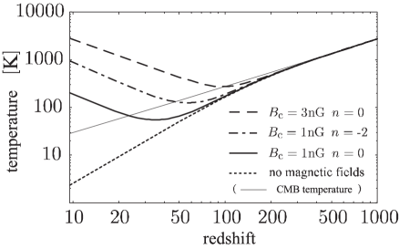
Figure 1: The evolutions of the hydrogen temperature. The dashed, dashed-dotted and solid lines are the hydrogen temperature for magnetic fields with $B_{\rm c}=3$nGauss and $n=0$, $B_{\rm c}=1$nGauss and $n=-2$ and $B_{\rm c}=1$nGauss and $n=0$. The dotted line is the hydrogen temperature in the standard cosmology (without magnetic fields) which is proportional to $(1+z)^{-2}$ once hydrogens decoupled with photons at $z\sim 200$. The thin solid line represents the CMB temperature which is proportional to $(1+z)^{-1}$.

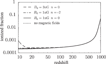
Figure 2: The evolution of the ionization fraction. The dashed, dashed-dotted and solid lines are the ionization fraction for magnetic fields with $B_{\rm c}=3$nGauss and $n=0$, $B_{\rm c}=1$nGauss and $n=-2$ and $B_{\rm c}=1$nGauss and $n=0$. The dotted line is the ionization fraction in the standard cosmology (without magnetic fields). In the neutral hydrogen number density, there is no significant change due to the energy diffusion of magnetic fields.

2.2 Generation of density fluctuations

Primordial magnetic fields generate the density fluctuations after recombination (Wasserman, 1978; Kim et al., 1996; Subramanian & Barrow, 1998; Gopal & Sethi, 2003; Sethi & Subramanian, 2005). The magnetic tension and pressure are more effective on small scales because the entanglements of magnetic fields are larger. Therefore, on small scales, the additional density power by magnetic fields is expected to dominate the primordial density power spectrum produced by inflation. The evolution equations of the density fluctuations with the primordial magnetic fields are described as,

$${\partial^{2}\delta_{\rm b}\over\partial t^{2}}=-2{\dot{a}\over a}{\partial\delta_{\rm b}\over\partial t}+4\pi G(\rho_{\rm b}\delta_{\rm b}+\rho_{\rm dm}\delta_{\rm dm})+S(t,{\bf x}),$$ (10)

$$S(t,{\bf x})={\nabla\cdot\left((\nabla\times{\bf B_{0}({\bf x})})\times{\bf B_{0}({\bf x})}\right)\over 4\pi\rho_{{\rm b}0}a^{3}(t)},$$ (11)

$${\partial^{2}\delta_{\rm dm}\over\partial t^{2}}=-2{\dot{a}\over a}{\partial\delta_{\rm dm}\over\partial t}+4\pi G(\rho_{\rm b}\delta_{\rm b}+\rho_{\rm dm}\delta_{\rm dm}),$$ (12)

where $\rho_{\rm dm}$ is the dark matter density, and $\delta_{\rm b}$ and $\delta_{\rm dm}$ are the density contrasts of baryons and dark matters, respectively.

In order to solve these equations, we define the total matter density $\rho_{\rm m}$ and the matter density contrast $\delta_{\rm m}$ as

$$\rho_{\rm m}\equiv\rho_{\rm b}+\rho_{\rm dm},$$ (13)

$$\delta_{\rm m}\equiv{(\rho_{\rm b}\delta_{\rm b}+\rho_{\rm dm}\delta_{\rm dm})\over\rho_{\rm m}}.$$ (14)

From Eqs. (10) and (12), the evolution of $\delta_{\rm m}$ is given by

$${\partial^{2}\delta_{\rm m}\over\partial t^{2}}=-2{\dot{a}\over a}{\partial\delta_{\rm m}\over\partial t}+4\pi G\rho_{\rm m}\delta_{\rm m}+{\rho_{\rm b}\over\rho_{\rm m}}S(t,{\bf x}).$$ (15)

The solution of Eq. (15) can be acquired by the Green’s function method,

$$\delta_{\rm m}=A({\bf x})D_{1}(t)+B({\bf x})D_{2}(t)-{\Omega_{\rm b}\over\Omega_{\rm m}}D_{1}(t)\int^{t}_{t_{\rm i}}dt^{\prime}{S(t^{\prime},{\bf x})D_{2}(t^{\prime})\over W(t^{\prime})}+{\Omega_{\rm b}\over\Omega_{\rm m}}D_{2}(t)\int^{t}_{t_{\rm i}}dt^{\prime}{S(t^{\prime},{\bf x})D_{1}(t^{\prime})\over W(t^{\prime})},$$ (16)

where $D_{1}(t)$ and $D_{2}(t)$ are the homogeneous solutions of Eq. (15) and $W$ is the Wronskian and is expressed as

$$W(t)=D_{1}(t)\dot{D}_{2}(t)-D_{2}(t)\dot{D}_{1}(t),$$ (17)

and $t_{\rm i}$ denotes the initial time.

The first and second terms of Eq. (16) correspond to the growing and the decaying mode solutions of primordial density fluctuations and the third and fourth terms are the ones generated by the primordial magnetic fields. We represent the former two terms as $\delta_{\rm mP}$ and the latter twos as $\delta_{\rm mM}$. Here we only consider the growing solution for $\delta_{\rm mP}$. The analytic solution of $\delta_{\rm mM}$ in the matter dominated epoch is obtained by Wasserman (1978) and Kim et al. (1996). In this paper, we concentrate on the evolution of fluctuations before reionization $z\ga 10$ when the universe is matter dominant and the contribution from the dark energy is negligible. Therefore we can utilize their solution. In the matter dominated epoch, $D_{1}(t)\propto t^{2/3}$ and $D_{2}(t)\propto t^{-1}$. Accordingly the terms generated by magnetic fields of Eq. (16) can be written as

$$\delta_{\rm mM}={\Omega_{\rm b}\over\Omega_{\rm m}}\left[{9\over 10}\left({t\over t_{\rm i}}\right)^{2/3}+{3\over 5}\left({t\over t_{\rm i}}\right)^{-1}-{3\over 2}\right]t_{\rm i}^{2}S(t_{\rm i},{\bf x}).$$ (18)

Once the density fluctuations were generated by the primordial magnetic fields, they grow due to the gravitational instability so that the growth rate is same as the primordial density fluctuations.

Next, we calculate the power spectrum of the matter density fluctuations. Assuming that there is no correlations between the magnetic fields and the primordial density fluctuations for simplicity, we can describe the matter power spectrum as

$$P_{\rm m}(k)=P_{\rm mP}(k)+P_{\rm mM}(k)\equiv\langle|\delta_{\rm mP}(k)|^{2}\rangle+\langle|\delta_{\rm mM}(k)|^{2}\rangle,$$ (19)

where $\delta_{\rm mP}(k)$ and $\delta_{\rm mM}(k)$ are the Fourier components of $\delta_{\rm mP}$ and $\delta_{\rm mM}$, respectively, and $\langle~{}\rangle$ denotes the ensemble average.

We numerically calculate $P_{\rm mP}(k)$ by using the CMBFAST code (Seljak & Zaldarriaga, 1996), while $P_{\rm mM}(k)$ is obtained from Eq. (18) as

$$P_{\rm mM}(k)=\left({\Omega_{\rm b}\over\Omega_{\rm m}}\right)^{2}\left(t_{\rm i}^{2}\over 4\pi\rho_{{\rm b}0}a^{3}(t_{\rm i})\right)^{2}\left[{9\over 10}\left({t\over t_{\rm i}}\right)^{2/3}+{3\over 5}\left({t\over t_{\rm i}}\right)^{-1}-{3\over 2}\right]^{2}I^{2}(k),$$ (20)

where

$$I^{2}(k)\equiv\langle|\nabla\cdot(\nabla\times{\bf B}_{0}({\bf x}))\times{\bf B}_{0}({\bf x})|^{2}\rangle.$$ (21)

Applying isotropic Gaussian statistics Eq (2), we can rewrite the nonlinear convolution Eq. (21) as

$$I^{2}(k)=\int dk_{1}\int d\mu{B^{2}_{0}(k_{1})B^{2}_{0}(|{\bf k-k_{1}}|)\over|{\bf k-k_{1}}|^{2}}\left[2k^{5}k_{1}^{3}\mu+k^{4}k_{1}^{4}(1-5\mu^{2})+2k^{3}k_{1}^{5}\mu^{3}\right],$$ (22)

where $\mu$ is $\mu={\bf k}\cdot{\bf k}_{1}/kk_{1}$. The integration of $I^{2}(k)$ is determined by the value of integrand at $k_{1}=k_{\rm c}$ and $|{\bf k_{1}-k}|=k_{\rm c}$ because the power spectrum $B_{0}^{2}(k)$ has the power law shape with sharp cutoff at $k=k_{\rm c}$. Note that the direct cascade process of the magnetic fields from large scales to small scales likely produces a power-law tail instead of sharp cutoff in the power spectrum above $k_{\rm c}$ as we discussed before. However, it is still true that most of the contribution on the integration $I^{2}(k)$ comes from the peak of the spectrum at $k_{\rm c}$ as well as the sharp cutoff case, although some corrections may be needed.

Let us introduce an important scale for the evolution of density fluctuations, i.e., the magnetic Jeans length. Below this scale, the magnetic pressure gradients, which we do not take into account in Eq. (15), counteract the gravitational force and prevent further evolution of density fluctuations. The magnetic Jeans scale $k_{\rm MJ}\sim v_{\rm A}/H$ is evaluated as (Kim et al., 1996)

$$k_{\rm MJ}=5\pi{\sqrt{\rho_{\rm m0}\rho_{\rm b0}G}\over B_{0}}=12.7{\rm Mpc}^{-1}\left({B_{0}\over 1{\rm nGauss}}\right)^{-1}\left({h^{2}\Omega_{\rm b}\over 0.0224}\right)^{1/2}\left({h^{2}\Omega_{\rm m}\over 0.135}\right)^{1/2}.$$ (23)

Here, the primordial magnetic fields have a power-low spectrum with spectral index $n$ and sharp cutoff at $k_{\rm c}$ so that the magnetic Jeans scale can be written from Eqs. (4) and (23) as

$$k_{\rm MJ}=\left({5\over 8\pi}\sqrt{3\over 2}\right)^{2/(n+5)}k_{\rm c}.$$ (24)

Baryon density fluctuations below the magnetic Jeans scale (the mode $k>k_{\rm MJ}$) oscillate and do not grow.

Using Eq. (22), we numerically calculate the matter power spectrum $P_{\rm m}(k)$. We show the evolution of $k^{3}P_{\rm m}(k)$ for the primordial magnetic fields with $B_{\rm c}=1$nGauss and $n=1$ in Fig. 3. The contribution from the density fluctuations generated by the primordial magnetic fields is dominated on small scales ($\la 100$kpc). Since the growth rates of both $P_{\rm mP}$ and $P_{\rm mM}$ are $t^{4/3}\propto 1/(1+z)^{2}$, the amplitude of the total matter power spectrum $P_{\rm m}$ is proportional to $1/(1+z)^{2}$ and the comoving scale on which $P_{\rm mM}$ starts to dominate $P_{\rm mP}$ stays constant ($k\sim 15{\rm Mpc}^{-1})$ as is shown in Fig. 3.

In Fig. 4, we plot the matter power spectra for models with different magnetic field amplitudes at $z=30$. We can analytically estimate Eq. (22) in the limit of $k/k_{\rm c}\ll 1$ as $I^{2}(k)\sim\alpha B_{\rm c}^{2n+10}k^{2n+7}+\beta B_{\rm c}^{7}k^{4}$ where $\alpha$ and $\beta$ are coefficients which depend on $n$ (Kim et al., 1996; Gopal & Sethi, 2003). Here we employ the fact that the cutoff scale $k_{\rm c}$ is proportional to $B^{-1}_{\rm c}$ as is shown in Eq. (4). The former term dominates if $n<-1.5$, while the latter one dominates for $n>-1.5$. Accordingly, the matter power spectrum, $k^{3}P_{\rm m}(k)$, is proportional to $B_{\rm c}^{2n+10}k^{2n+7}$ for $n<-1.5$ or to $B_{\rm c}^{7}k^{4}$ for $n>-1.5$. These dependences of $k^{3}P_{\rm m}(k)$ on $B_{\rm c}$ and $n$ can be found in Fig. 4.

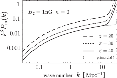
Figure 3: The redshift evolution of the matter power spectrum for the model with $B_{\rm c}=1$nGauss and $n=0$. The dashed, dotted and solid lines represent the matter power spectrum at $z=20$, $z=30$ and $z=40$ (from top to bottom). The thin solid line is the matter power spectrum without magnetic fields at $z=40$.

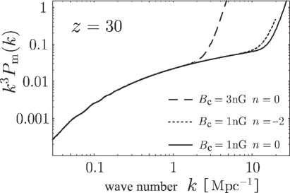
Figure 4: The matter power spectra for models with different magnetic field strengths. The dashed, dotted and solid lines are the power spectra with the primordial magnetic fields $B_{\rm c}=3$nGauss and $n=0$, $B_{\rm c}=1$nGauss and $n=-2$ and $B_{\rm c}=1$nGauss and $n=0$ (from top to bottom) at $z=30$.

3 brightness temperature fluctuations by the 21cm line

In this section, we discuss the calculation of the CMB brightness temperature fluctuations generated by the hydrogen 21cm line and the angler power spectrum of them. First, let us discuss the spin temperature on which the amplitude of the brightness temperature fluctuations depends. The spin temperature is defined through the ratio of the number density of hydrogen atoms between in the excited state and in the ground state of the 21cm transition,

$${n_{1}\over n_{0}}=3\exp\left(-{T_{*}\over T_{\rm s}}\right),$$ (25)

where subscripts 1 and 0 denote the excited and ground states and $T_{*}$ corresponds to the energy difference between these states, $T_{*}=0.0682$K. The factor 3 in Eq. (25) comes from the ratio of the spin degeneracy factors. The evolution of the number density of hydrogen atoms in the ground state is described as

$${\partial n_{0}\over\partial z}-{3\over 1+z}n_{0}=-{1\over(1+z)H(z)}\left[-n_{0}\left(C_{01}+B_{01}I_{\nu}\right)+n_{1}\left(C_{10}+A_{10}+B_{10}I_{\nu}\right)\right],$$ (26)

where $C_{01}$ and $C_{10}$ are the collisional excitation and de-excitation rate coefficients, $A_{10}$ is the Einstein A-coefficient, $B_{01}$ and $B_{10}$ are the Einstein B-coefficients and $I_{\nu}$ is the specific intensity of CMB at frequency $\nu$. The collisional de-excitation coefficient is written as $C_{10}=4\kappa_{10}(T_{\rm k})n_{\rm H}/3$ where $n_{\rm H}\equiv n_{0}+n_{1}$ is the neutral hydrogen number density and $\kappa_{10}(T_{\rm k})$ is tabulated as a function of the hydrogen temperature $T_{\rm k}$ (Allison & Dalgarno, 1969). Typically $\kappa_{10}(T_{\rm k})$ is order $10^{-10}{\rm cm}^{3}{\rm s}^{-1}$ in $T_{\rm k}<1000$K. The excitation coefficient is related with the de-excitation coefficient by the detailed balance as $C_{01}=C_{10}\exp(-2\pi\hbar\nu/kT_{\rm k})$. The Einstein coefficients are coupled by the Einstein relations as

$$B_{01}=3B_{10}=\left(3c^{2}\over 4\pi\hbar\nu^{3}\right)A_{10},$$ (27)

where $A_{10}=2.85\times 10^{-15}{\rm s}^{-1}$. The evolution of the number density of the excited hydrogen atoms is also written as

$${\partial n_{1}\over\partial z}-{3\over 1+z}n_{1}=-{1\over(1+z)H(z)}\left[n_{0}\left(C_{01}+B_{01}I_{\nu}\right)-n_{1}\left(C_{10}+A_{10}+B_{10}I_{\nu}\right)\right].$$ (28)

From Eqs. (25), (26) and (28), we can derive the evolution of the spin temperature

$${\partial\over\partial z}\left(1\over T_{\rm s}\right)=-{4\over(1+z)H(z)}\left[\left({1\over T_{\rm k}}-{1\over T_{\rm s}}\right)C_{10}+\left({1\over T_{\gamma}}-{1\over T_{\rm s}}\right){T_{\gamma}\over T_{*}}A_{10}\right],$$ (29)

where we employ the approximation $\exp(-T_{*}/T)\approx 1-T_{*}/T$, and the Rayleigh-Jeans law, $I_{\nu*}=2\nu_{*}^{2}k_{\rm B}T_{\gamma}/c^{2}$ with $\nu_{*}\equiv k_{\rm B}T_{*}/(2\pi\hbar)$ because we are interested in the epoch when $T_{\rm s}$, $T_{\rm k}$, $T_{\gamma}\gg T_{\rm*}$.

The emission and absorption of the 21cm line from neutral hydrogens affect the CMB brightness temperature at the frequency $\nu_{*}/(1+z)$ by

$$T_{\rm b}\left({\nu_{*}\over(1+z)},{\bf\hat{n}}\right)=\tau{T_{\rm s}-T_{\gamma}\over 1+z},$$ (30)

where ${\bf\hat{n}}$ is a unit direction vector and $\tau$ is the optical depth of the 21cm line,

$$\tau={3\pi c^{3}n_{\rm H}\hbar A_{10}\over 16\nu_{*}^{2}k_{\rm B}T_{\rm S}}{1\over H(z)}.$$ (31)

The fluctuations of the brightness temperature at the frequency $\nu_{*}/(1+z)$ are obtained from Eq. (30) as

$$\delta T_{\rm b}\left({\nu_{*}\over(1+z)},{\bf\hat{n}}\right)={\tau\over 1+z}\left[\left(T_{\rm s}-T_{\gamma}\right)\delta_{\rm m}+T_{\gamma}{\delta T_{\rm s}\over T_{\rm s}}\right],$$ (32)

where we ignore the fluctuations of the CMB temperature and the ionization fraction and we assume that the hydrogen number density contrast is corresponding to the matter density contrast. From Eq. (32), it is found that the brightness temperature fluctuations at the frequency $\nu_{*}/(1+z)$ are determined by the density and the spin temperature fluctuations at redshift $z$. Note that we ignore the effect of the line-of-sight component of the neutral hydrogen’s peculiar velocity. The line-of-sight component of the peculiar velocity affects the optical depth through the distortion of the redshift space. The contribution from the peculiar velocity could be substantially large on very large scales (for details, see Bharadwaj & Ali 2004), while it is negligible on scales comparable to the future observations’ survey area. Therefore we ignore the term of the peculiar velocity.

In order to calculate Eq. (32), we need to know the time evolution of the spin temperature fluctuations. The evolution equation can be obtained from Eq (29) as

$${\partial\over\partial z}\left({\delta T_{\rm s}\over T_{\rm s}}\right)={4T_{\rm s}\over H(z)(1+z)}\left[\left({C_{10}\over T_{\rm k}}+{A_{10}\over T_{*}}\right){\delta T_{\rm s}\over T_{\rm s}}+\left({1\over T_{\rm k}}-{1\over T_{\rm s}}\right)C_{10}{\delta n_{\rm H}\over n_{\rm H}}+\left(\left({1\over T_{\rm k}}-{1\over T_{\rm s}}\right){\partial\ln\kappa\over\partial\ln T_{\rm k}}-{1\over T_{\rm k}}\right)C_{10}{\delta T_{\rm k}\over T_{\rm k}}\right],$$ (33)

where we ignore the fluctuations of the CMB temperature and the ionization fraction. Because of the energy pumping from CMB, strictly speaking, the ordinary adiabatic relation, i.e. $\delta T_{\rm k}/T_{\rm k}=(\gamma-1)\delta n_{\rm H}/n_{\rm H}$ where $\gamma$ is adiabatic index and $\gamma=5/3$, is broken. However, Bharadwaj & Ali (2004) have shown that the adiabatic relation is still valid until the star formation process proceeds. Hence, hereafter, we assume $\delta T_{\rm k}/T_{\rm k}=(\gamma-1)\delta n_{\rm H}/n_{\rm H}$ in Eq. (33).

Let us calculate the angular power spectrum of brightness temperature fluctuations $C_{l}(\nu_{*}/(1+z))$. We can expand the brightness temperature fluctuations $\delta T_{\rm b}\left(\nu_{*}/(1+z),{\bf\hat{n}}\right)$ into spherical harmonics with the expansion coefficients $a_{lm}$. Accordingly the angular power spectrum $C_{l}(\nu_{*}/(1+z))=\left\langle|a_{lm}|^{2}\right\rangle$ can be written as

$$C_{l}\left(\nu_{*}\over(1+z)\right)=\langle|a_{lm}|^{2}\rangle=4\pi\int{dk^{3}\over(2\pi)^{3}}\left\langle|\delta T_{\rm b}\left({\nu_{*}\over(1+z)},k\right)|^{2}\right\rangle j_{l}^{2}(k(\eta_{0}-\eta(z))),$$ (34)

where $j_{l}(x)$ is the spherical bessel function, $\eta$ is the conformal time and $\delta T_{\rm b}(\nu,k)$ is the Fourier component of $\delta T_{\rm b}$ at the frequency $\nu$ which is calculated by Eq. (32).

4 results and discussion

We can calculate the angular power spectrum of the brightness temperature fluctuations produced by the 21cm line with the existence of the primordial magnetic fields from Eq. (34). In this section, we show the evolution of the spin temperature and the angular power spectrum for three different primordial magnetic fields, i.e., $(B_{\rm c},~{}n)=(1{\rm nGauss},~{}0)$, $(1{\rm nGauss},~{}-2)$, and $(3{\rm nGauss},~{}0)$.

First we discuss the effect of the primordial magnetic fields on the spin temperature. Fig. 5 shows the redshift evolution of the spin temperature. The spin temperature is well approximated to the steady state of Eq. (29) as (Field, 1959)

$$T_{\rm s}={T_{\gamma}+yT_{\rm k}\over 1+y},$$ (35)

where $y$ is the collisional efficiency and written as

$$y={2\pi\hbar\nu_{*}C_{10}\over k_{\rm B}T_{\rm k}A_{10}}.$$ (36)

The behaviors of the spin temperature in Fig. 5 can be explained by Eq. (35). In the high redshift ($z>100$), because the collisional efficiency $C_{10}$ is high ($y\gg 1$) so that the spin temperature couples the hydrogen temperature, i.e., $T_{\rm s}\simeq T_{\rm k}$. As the universe expands the collisional efficiency becomes low ($y\ll 1$) so that the spin temperature approaches the CMB temperature $T_{\rm s}\simeq T_{\gamma}$. The primordial magnetic fields make the hydrogen temperature increase due to the dissipation. The collisional efficiency increases as the hydrogen temperature increases. Accordingly the combination $yT_{\rm K}$ in the numerator of Eq. (35) increases although $y$ decreases. Therefore the spin temperature becomes higher than the one without the magnetic fields. If the primordial magnetic fields are strong enough, the hydrogen and spin temperatures can exceed the CMB temperature as is shown in Fig. 5.

Next, let us show the angler power spectra of the brightness temperature fluctuations by the 21cm line for the various primordial magnetic fields in Fig. 6. For reference, we plot the angler power spectra without magnetic fields, which are consistent with previous works by Bharadwaj & Ali (2004).

The primordial magnetic fields affect the overall amplitude of the angular power spectrum and the shape of the angular power spectrum on large $l$’s. The modification on the shape of the angular power spectrum is caused by the density fluctuations generated by the magnetic fields on small scales. From Eq. (32), the brightness temperature fluctuations are determined by the density fluctuations $\delta_{\rm m}$ and the spin temperature fluctuations $\delta T_{\rm s}/T_{\rm s}$. Applying the steady state approximation and $y\ll 1$ to Eq. (33), we can obtain $\delta T_{\rm s}/T_{\rm s}$ in the leading order of $y$ as

$${\delta T_{\rm s}\over T_{\rm s}}=y\left({T_{\rm k}\over T_{\rm\gamma}}-\gamma\right)\delta_{\rm m},$$ (37)

where we ignore the temperature derivative term of $\kappa$ and substitute $T_{\rm s}$ with Eq. (35). Accordingly Eq. (32) leads to

$$\delta T_{\rm b}={\tau\over 1+z}y\left[2T_{\rm k}-(1+\gamma)T_{\gamma}\right]\delta_{\rm m}.$$ (38)

It turns out that the brightness temperature fluctuations are simply proportional to the density fluctuations. Therefore the additional “blue” density power spectrum produced by the primordial magnetic fields on small scales appears as the “blue” angler power spectrum on large $l$’s. The magnetic Jeans scale corresponds to $l_{\rm MJ}\sim 3\times 10^{5}(1{\rm nGauss}/B_{\rm c})$. The angular power spectrum $C_{l}$ increases until $l_{\rm MJ}$ and starts to show the oscillatory behavior above $l>l_{\rm MJ}$.

The evolution of the power spectrum amplitude with the primordial magnetic fields is classified into two regimes: $T_{\gamma}>T_{\rm s}$ and $T_{\gamma}<T_{\rm s}$. In $T_{\gamma}>T_{\rm s}$, neutral hydrogens absorb the CMB photons while neutral hydrogens emit the 21cm line into CMB in $T_{\gamma}<T_{\rm s}$. If there is no magnetic fields, $T_{\gamma}>T_{\rm s}$ until the formation process of stars and galaxies takes place. On the other hand, the dissipation of the primordial magnetic fields makes the hydrogen temperature higher than the CMB temperature and $T_{\rm s}$ can exceed $T_{\gamma}$ at high redshift as mentioned above.

In the regime of $T_{\gamma}>T_{\rm s}$, the amplitude of the angular power spectrum with the primordial magnetic fields declines as is the case with no magnetic fields due to the fact that $T_{\rm s}$ approaches to $T_{\gamma}$. However, the decline of the power spectrum is more prominent for the model with the primordial magnetic fields (see bold and thin solid lines on the top and middle panels of FIG. 6). The reason is following. For the model without magnetic fields, $T_{\gamma}\gg T_{\rm k}$. From Eq. (38), therefore, the angular power spectrum $C_{l}\propto|(1+\gamma)T_{\gamma}|^{2}$. If the primordial magnetic fields exist, on the other hand, $T_{\rm k}$ increases due to the dissipation. Accordingly $C_{l}\propto|(1+\gamma)T_{\gamma}-2T_{\rm k}|^{2}<|(1+\gamma)T_{\gamma}|^{2}$ as far as $T_{\rm k}<(1+\gamma)T_{\gamma}$. Therefore the suppression of the angular power spectrum of the model with the primordial magnetic fields is more prominent.

Once the hydrogen temperature $T_{\rm k}$ exceeds the CMB temperature $T_{\gamma}$ (or equivalently $T_{\rm s}>T_{\gamma}$), the amplitude of the brightness temperature fluctuations starts growing as the universe evolves. In the low redshift universe, the hydrogen temperature becomes high enough that we can assume the CMB temperature is negligible to the hydrogen temperature, $T_{\gamma}\ll T_{\rm k}$. Hence the fluctuations of the brightness temperature can be approximated as

$$\delta T_{\rm b}={\tau\over 1+z}2yT_{\rm k}\delta_{\rm m}.$$ (39)

Perhaps one might think that the amplitude of the magnetic fields can be determined by measuring the angular power spectrum since $T_{\rm k}$ depends on the amplitude. However it is not the case. Because $y$ is related to the hydrogen temperature through $C_{10}/T_{\rm k}$, the overall dependence of $\delta T_{\rm b}$ on the hydrogen temperature comes from $C_{10}$. In $\delta T_{\rm b}>100$K, $C_{10}$ is not a strong function of the hydrogen temperature. Accordingly, the amplitude of the angular spectrum does not depend much on the strength of the primordial magnetic fields as is shown in Fig. 6. Therefore, in the regime of $T_{\gamma}<T_{\rm s}$, we can only measure the strength of the primordial magnetic fields through the turnover of the spectrum on high $l$’s.

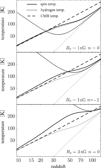
Figure 5: The evolution of the spin temperature. The solid lines, the dotted and dashed lines denote the spin temperature, the hydrogen temperature and the CMB temperature, respectively. We show these temperature for three different magnetic field spectra: $B_{\rm c}=1$nGauss and $n=0$, $B_{\rm c}=1$nGauss and $n=-2$ and $B_{\rm c}=3$nGauss and $n=0$ (from top panel to bottom panel). For reference, we plot the spin temperature and the hydrogen temperature in the standard cosmology with no primordial magnetic fields as the thin solid lines and dotted lines. In all cases, the spin temperature closes in the hydrogen temperature in high redshift and approaches the CMB temperature asymptotically.

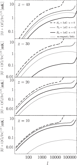
Figure 6: The angler power spectra of CMB brightness temperature fluctuations by the 21cm line at the frequency $v_{*}/(1+z)$ for $z=40,30,20$, and $10$ from the top to bottom panels, respectively. The dashed, dotted and solid lines represent the spectra for the models with $B_{\rm c}=3$nGauss and $n=0$, $B_{\rm c}=1$nGauss and $n=-2$ and $B_{\rm c}=1$nGauss and $n=0$, respectively. The thin solid line in each panel is the spectrum of the model without the magnetic fields.

5 summary

In this paper we investigate the effect of the primordial magnetic fields on the CMB brightness temperature fluctuations produced by the hydrogen 21cm line.

The brightness temperature fluctuations depend on the density fluctuations, the hydrogen temperature and the ionization fraction whose evolutions are affected by the primordial magnetic fields: the dissipation of the magnetic field energy works as heat source and the Lorentz force generates the density fluctuations after recombination. The primordial magnetic fields with nano Gauss strength can heat hydrogens up to several thousands degrees Kelvin by the ambipolar diffusion and produce dominant additional “blue power” in the matter density spectrum on scales smaller than $100$kpc.

Through these effects, the primordial magnetic fields modify the angular power spectrum of the brightness temperature fluctuations. First, an additional blue spectrum can be found due to the existence of the blue power in the matter density spectrum. Secondly, the overall amplitude of the angular spectrum can be modified by the magnetic fields. If the hydrogen temperature is lower than the CMB temperature, the amplitude becomes smaller than the one without magnetic fields. The difference depends on the hydrogen temperature. On the other hand, if the hydrogen temperature becomes higher than the CMB temperature, the amplitude of the angular power spectrum, which depends little on the magnetic field amplitude in this case, exceeds the one without magnetic fields.

Perhaps each feature of the brightness temperature fluctuations is not a direct evidence for the existence of the primordial magnetic fields. Possible existence of the isocurvature mode on small scales can also boost the spectrum on small scales, while the higher hydrogen temperature might be achieved by the other heat source, e.g., the decaying dark matter. However, both blue spectrum and modification of overall amplitude of the angular power spectrum may provide a unique evidence for the existence of the primordial magnetic fields. Or at least we can set a stringent constraint on the shape and the amplitude of the primordial magnetic fields.

In this paper, we ignore the reionization process due to the ordinary astronomical objects, i.e., stars, which provides a significant impact on the brightness temperature fluctuations, since we are focus on the epoch before reionization. The reionization can be as late as $z\sim 9$ from the latest WMAP results (Spergel et al., 2006). Once the reionization process starts, the ionizing UV photons produced by stars make the hydrogen temperature high and the Ly-$\alpha$ pumping of the hydrogen 21cm transitions efficient. Accordingly, the coupling between the spin temperature and the hydrogen temperature becomes stronger. This reionization process could be also affected by the primordial magnetic fields due to the modification of the matter power spectrum which induces the star formation (Tashiro & Sugiyama, 2006). Therefore we need to consider the reionization process with the primordial magnetic fields in order to investigate the role of the magnetic fields below $z\la 10$, which is beyond the scope of this paper.

References

- Adams et al. (1996) Adams J., Danielsson U. H., Grasso D., Rubinstein H., 1996, Phys. Lett. B, 388, 253
- Ali et al. (2005) Ali S. S., Bharadwaj S., Pandey B., 2005, MNRAS, 363, 251
- Allison & Dalgarno (1969) Allison A. C., Dalgarno A., 1969, ApJ, 158, 423
- Banerjee & Jedamzik (2004) Banerjee R., Jedamzik K., 2004, Phys. Rev. D, 70, 123003
- Barrow et al. (1997) Barrow J. D., Ferreira P. G., Silk J., 1997, Phys. Rev. Lett., 78, 3610
- Bharadwaj & Ali (2004) Bharadwaj S., Ali S. S., 2004, MNRAS, 352, 142
- Biermann (1950) Biermann L., 1950, Z. Naturforsch., 5
- Cheng et al. (1996) Cheng B., Olinto A. V., Schramm D. N., Truran J. W., 1996, Phys. Rev. D, 54, 4714
- Cooray (2005) Cooray A., 2005, MNRAS, 363, 1049
- Cowling (1956) Cowling T. G., 1956, MNRAS, 116, 114
- Draine et al. (1983) Draine B. T., Roberge W. G., Dalgarno A., 1983, ApJ, 264, 485
- Field (1959) Field G. B., 1959, ApJ, 129, 536
- Giovannini (2004) Giovannini M., 2004, International Journal of Modern Physics D, 13, 391
- Gopal & Sethi (2003) Gopal R., Sethi S. K., 2003, Journal of Astrophysics and Astronomy, 24, 51
- Jedamzik et al. (1998) Jedamzik K., Katalinić V., Olinto A. V., 1998, Phys. Rev. D, 57, 3264
- Jedamzik et al. (2000) Jedamzik K., Katalinić V., Olinto A. V., 2000, Phys. Rev. Lett., 85, 700
- Kernan et al. (1996) Kernan P. J., Starkman G. D., Vachaspati T., 1996, Phys. Rev. D, 54, 7207
- Kim et al. (1996) Kim E.-J., Olinto A. V., Rosner R., 1996, ApJ, 468, 28
- Kim et al. (1990) Kim K.-T., Kronberg P. P., Dewdney P. E., Landecker T. L., 1990, ApJ, 355, 29
- Kim et al. (1991) Kim K.-T., Kronberg P. P., Tribble P. C., 1991, ApJ, 379, 80
- Kosowsky et al. (2005) Kosowsky A., Kahniashvili T., Lavrelashvili G., Ratra B., 2005, Phys. Rev. D, 71, 043006
- Kronberg (1994) Kronberg P. P., 1994, Reports of Progress in Physics, 57, 325
- Kronberg et al. (1992) Kronberg P. P., Perry J. J., Zukowski E. L. H., 1992, ApJ, 387, 528
- Lewis (2004) Lewis A., 2004, Phys. Rev. D, 70, 043011
- Loeb & Zaldarriaga (2004) Loeb A., Zaldarriaga M., 2004, Phys. Rev. Lett., 92, 211301
- Mack et al. (2002) Mack A., Kahniashvili T., Kosowsky A., 2002, Phys. Rev. D, 65, 123004
- Peebles (1968) Peebles P. J. E., 1968, ApJ, 153, 1
- Peebles (1993) Peebles P. J. E., 1993, Principles of physical cosmology, Princeton University Press, 1993
- Scóccola et al. (2004) Scóccola C., Harari D., Mollerach S., 2004, Phys. Rev. D, 70, 063003
- Seager et al. (1999) Seager S., Sasselov D. D., Scott D., 1999, ApJL, 523, L1
- Seljak & Zaldarriaga (1996) Seljak U., Zaldarriaga M., 1996, ApJ, 469, 437
- Sethi & Subramanian (2005) Sethi S. K., Subramanian K., 2005, MNRAS, 356, 778
- Tashiro & Sugiyama (2006) Tashiro H., Sugiyama N., 2006, MNRAS, 368, 965
- Spergel et al. (2003) Spergel D. N., Verde L., Peiris H. V., Komatsu E. et al., 2003, ApJS, 148, 175
- Spergel et al. (2006) Spergel D. N., Bean R., Dore’ O., Nolta M. R. et al., 2006, astro-ph/0603449
- Subramanian & Barrow (1998) Subramanian K., Barrow J. D., 1998, Phys. Rev. D, 58, 083502
- Subramanian et al. (2003) Subramanian K., Seshadri T. R., Barrow J. D., 2003, MNRAS, 344, L31
- Tashiro et al. (2005) Tashiro H., Sugiyama N., Banerjee R., 2005, Phys. Rev. D, 73, 023002
- Voronov (1997) Voronov G. S., 1997, Atomic Data and Nuclear Data Tables, 65, 1
- Wasserman (1978) Wasserman I., 1978, ApJ, 224, 337
- Widrow (2002) Widrow L. M., 2002, Reviews of Modern Physics, 74, 775
- Yamazaki et al. (2005) Yamazaki D. G., Ichiki K., Kajino T., 2005, ApJ, 625, L1