Atmosphere Models of Magnetized Neutron Stars: QED Effects, Radiation Spectra and Polarization Signals

Abstract

Observations of surface emission from isolated neutron stars (NSs) provide unique challenges to theoretical modeling of radiative transfer in magnetized NS atmospheres. Recent work has demonstrated the critical role of vacuum polarization effects in determining NS spectra and polarization signals, in particular the conversion of photon modes (due to the “vacuum resonance” between plasma and vacuum polarization) propagating in the density gradient of the NS atmosphere. Previous NS atmosphere models incorporated the mode conversion effect approximately, relying on transfer equations for the photon modes. Such treatments are inadequate near the vacuum resonance, particularly for magnetic field strengths around $B\sim B_{l}\simeq 7\times 10^{13}$ G, where the vacuum resonance occurs near the photosphere. In this paper, we provide an accurate treatment of the mode conversion effect in magnetized NS atmosphere models, employing both the modal radiative transfer equations coupled with an accurate mode conversion probability at the vaccum resonance, and the full evolution equations for the photon Stokes parameters. In doing so, we are able to quantitatively calculate the effects of vacuum polarization on atmosphere structure, emission spectra and beam patterns, and polarizations for the entire range of magnetic field strengths, $B=10^{12}-10^{15}$ G. In agreement with previous works, we find that for NSs with magnetic field strength $B\ga 2\,B_{l}$, vacuum polarization reduces the widths of spectral features, and softens the hard spectral tail typical of magnetized atmosphere models. For $B\la B_{l}/2$, vacuum polarization does not change the emission spectra, but can significantly affect the polarization signals. Our new, accurate treatment of vacuum polarization is particularly important for quantitative modeling of NS atmospheres with “intermediate” magnetic fields, $B\simeq(0.5-2)\,B_{l}$. We provide fitting formulae for the temperature profiles for a suite of NS atmosphere models with different field strengths, effective temperatures and chemical compositions (ionized H or He). These analytical profiles are useful for direct modeling of various observed properties of NS surface emission. As an example, we calculate the observed intensity and polarization lightcurves from a rotating NS hotspot, taking into account the evolution of photon polarization in the magnetosphere. We show that vacuum polarization induces a unique energy-dependent linear polarization signature, and that circular polarization can be generated in the magnetosphere of rapidly rotating NSs. We discuss the implications of our results to recent observations of thermally emitting isolated NSs and magnetars, as well as the prospects of future spectral and polarization observations.

1 Introduction

Thermal surface emission from isolated neutron stars (NSs) (e.g., Kaspi et al., 2005) can potentially provide invaluable information on the physical properties and evolution of NS equations of state at super-nuclear densities, cooling histories, magnetic fields, and surface compositions (see, e.g., Prakash et al. 2001; Yakovlev & Pethick 2004 for review). In recent years, significant progress has been made in detecting such radiation using X-ray telescopes such as Chandra and XMM-Newton. For example, the spectra of a number of radio pulsars (PSR B1055-52, B0656+14, Geminga and Vela) have been observed to possess thermal components that can be attributed to emission from NS surfaces and/or heated polar caps (see, e.g., Becker & Pavlov 2002). Phase-resolved spectroscopic observations have become possible, revealing the surface magnetic field geometry and emission radius of the pulsar (e.g., Caraveo et al. 2004; De Luca et al. 2005; Jackson & Halpern 2005). Chandra has also uncovered a number of compact sources in supernova remnants with spectra consistent with thermal emission from NSs (see Pavlov et al. 2003), and useful constraints on NS cooling physics have been obtained (Slane et al. 2002; Yakovlev & Pethick 2004).

Surface X-ray emission has also been detected from a number of soft gamma-ray repeaters (SGRs) and anomalous X-ray pulsars (AXPs) — these are thought to be magnetars, which emit radiation powered by the decay of superstrong ($B\mathrel{\raise 1.29167pt\hbox{$>$}\mkern-14.0mu\lower 2.58334pt\hbox{$\sim$}}10^{14}$ G) magnetic fields (see Thompson & Duncan 1995,1996; Woods & Thompson 2005). The quiescent magnetar emission consists of a blackbody-like component with temperature (3–7) $\times 10^{6}$ K, and a power-law tail from $2-10$ keV with photon index $2-3.5$ (e.g., Juett et al 2002; Kulkarni et al. 2003; Tiengo et al. 2005), as well as significant flux at $\sim 100$ keV (Kuiper et al. 2004; Kuiper et al. 2006). Somewhat surprisingly, the observed thermal emission does not show any of the spectral features one might expect, such as the ion cyclotron line around 1 keV (for typical magnetar field strengths).

The seven isolated, radio-quiet NSs (the so-called “dim isolated NSs”; see Haberl 2005) are also of great interest. These NSs share the property that their spectra appear to be entirely thermal, indicating that the emission arises directly from the NS atmospheres, uncontaminated by magnetospheric processes. The true nature of these sources is unclear at present: they could be young cooling NSs, or NSs kept hot by accretion from the ISM, or magnetars and their descendants (see van Kerkwijk & Kulkarni 2001, Mori & Ruderman 2003; Haberl 2005; Kaspi et al. 2005). While the brightest of these, RX J1856.5-3754, has a featureless spectrum remarkably well described by a blackbody (Drake et al. 2002; Burwitz et al. 2003), absorption lines/features at $E\simeq 0.2$–$2$ keV have recently been detected from at least four sources, including 1E 1207.4-5209 (at 0.7 and 1.4 keV, possibly also 2.1, 2.8 keV; Sanwal et al. 2002; Bignami et al. 2003; DeLuca et al. 2004; Mori et al. 2005), RX J1308.6+2127 (0.2-0.3 keV; Haberl et al. 2003), RX J1605.3+3249 (0.45 keV; van Kerkwijk et al. 2004), RX J0720.4$-$3125 (0.27 keV; Haberl et al. 2004a), and possibly several additional sources (see Haberl et al., 2004b; Zane et al., 2005). The identification of these features remains uncertain, with suggestions ranging from electron/ion cyclotron lines to atomic transitions of H, He or mid-Z atoms in a strong magnetic field (Ho & Lai 2004; Pavlov & Bezchastnov 2005; Mori et al. 2005). These sources also have different X-ray lightcurves: for example, RX J1856.5-3754 and RX J1605+3249 show no variability (pulse fraction $\mathrel{\raise 1.29167pt\hbox{$<$}\mkern-14.0mu\lower 2.58334pt\hbox{$\sim$}}1$-$3\%$), while RX J0720-3125 shows single-peaked pulsations ($P=3.39$ s) of amplitude $\sim 11\%$, with the spectral hardness and line width varying with the pulse phase, and RX J1308+2127 shows double-peaked pulsations ($P=10.3$ s) with amplitude $\sim 18\%$. Another puzzle concerns the optical emission: for at least four of these sources, optical counterparts have been identified, however, the optical flux is larger (by a factor of $4$-$10$) than the extrapolation from the blackbody fit to the X-ray spectrum (see, e.g., Trümper et al., 2004; Haberl, 2005).

The spectrum of NS thermal radiation is formed in the atmosphere layer (with scale height $\sim 0.1-10$ cm and density $10^{-3}-10^{3}$ g cm^-3) that covers the stellar surface. Thus, to properly interpret observations of NS surface emission, detailed modeling of NS atmospheres in strong magnetic fields is required.

1.1 Previous work on magnetic neutron star atmosphere models

The first magnetic NS atmosphere models were constructed by Shibanov et al. (1992) (see also Pavlov et al., 1995; Rajagopal et al., 1997; Zavlin & Pavlov, 2002), who focused on moderate field strengths $B\sim 10^{12}$–$10^{13}$ G and assumed full ionization (see also Zane et al. 2000 for atmosphere models with accretion). Similar ionized models for the magnetar field regime ($B\mathrel{\raise 1.29167pt\hbox{$>$}\mkern-14.0mu\lower 2.58334pt\hbox{$\sim$}}10^{14}$ G) were studied by Zane et al. (2001), Özel (2001) and Ho & Lai (2001,2003). An inaccurate treatment of the free-free opacities in the earlier models (Pavlov et al. 1995) was corrected by Potekhin & Chabrier (2003), and the correction has been incoporated into later models (Ho et al. 2003,2004). Recent works (Lai & Ho 2002,2003a; Ho & Lai 2003) have shown that in the magnetar field regime, the effect of strong-field quantum electrodynamics significantly influences the emergent atmosphere spectrum. In particular, vacuum polarization gives rise to a resonance phenomenon, in which photons can convert from the high-opacity mode to the low-opacity one and vice versa. This vacuum resonance tends to soften the hard spectral tail due to the non-greyness of the atmosphere and suppress the width of absoprtion lines (see Lai & Ho 2003a for a qualitative explanation). Even for modest field strengths ($B\mathrel{\raise 1.29167pt\hbox{$<$}\mkern-14.0mu\lower 2.58334pt\hbox{$\sim$}}10^{14}$ G), vacuum polarization can still leave a unique imprint on the X-ray polarization signal (Lai & Ho 2003b).

Because a strong magnetic field greatly increases the binding energies of atoms, molecules and other bound species (see Lai 2001), these bound states may have appreciable abundances in the NS atmosphere (Lai & Salpeter 1997; Potekhin et al. 1999). Early considerations of partially ionized atmospheres (e.g., Rajagopal et al., 1997) relied on oversimplified treatments of atomic physics (e.g., ionization equilibrium and equation of state) and nonideal plasma effects in strong magnetic fields. Recently, a thermodynamically consistent equation of state and opacities for magnetized ($B=10^{12}-10^{15}$ G), partially ionized H plasma have been obtained (Potekhin et al. 1999; Potekhin & Chabrier 2003,2004), and the effect of bound atoms on the dielectric tensor of the plasma has also be studied (Potekhin et al. 2004). These improvements have been incorporated into partially ionized, magnetic NS atmosphere models (Ho et al. 2003; Potekhin et al. 2004). Finally, for sufficiently low temperatures and/or strong magnetic fields, the NS atmosphere may undergo a phase transition into a condensed state (see Ruderman, 1971; Jones, 1986; Neuhauser et al., 1987; Lai & Salpeter, 1997; Lai, D., 2001; Medin & Lai, 2006a, b). Thermal emission from such a condensed surface has been studied by van Adelsberg et al. (2005) (cf. Turolla et al. 2004; Perez-Azorin et al. 2005).

1.2 This paper

While previous works have identified the importance and trend of the vacuum polarization effect (Lai & Ho 2002,2003a), the implementation of the effect in NS atmosphere models (Ho & Lai 2003,2004) has been based on approximations (see §2). So far all studies of magnetic NS atmospheres have relied on solving the transfer equations for the specific intensities of the two photon modes. As discussed in Lai & Ho (2003a) and reviewed in §2 below, these equations cannot properly handle the vacuum-induced mode conversion phenomenon because mode conversion intrinsically involves interference between different modes.

In this paper we provide a new, quantitatively accurate treatment of vacuum polarization effects in radiation transfer for fully ionized NS atmospheres. Our work confirms the semi-quantitative results obtained in previous works based on an approximate treatment of vacuum resonance (Ho & Lai 2003; Lai & Ho 2003b). Moreover, our new treatment allows us to quantitatively predict the spectral and polarization properties of NS atmospheres with field strengths varying from $10^{12}$ G to $10^{15}$ G.

The remainder of our paper is organized as follows: §2 describes the basic physics of vacuum polarization in radiative transfer and resonant mode conversion; §3 details two methods of solving the radiative transfer problem and our basic physics inputs, as well as tests of our numerical method; §4 presents the basic results from our models, including atmosphere structures (with fitting formulae for the temperature profiles), spectra, and emission beam patterns; §5 considers the observed polarization signals of atmosphere emission for a simple geometry (i.e., a rotating NS hotspot); and §6 discusses the implications of our results.

2 Effect of Vacuum Polarization on Radiative Transfer

Before describing our quantitative treatment of the vacuum polarization effect in NS atmospheres, it is useful to summarize the basic physics of the effect (see also Lai & Ho 2003a) and discuss the limitations of previous treatments.

Photons (with energy $E\ll E_{Be}=\hbar eB/m_{e}c$, the electron cyclotron energy) in magnetized NS atmospheres usually propagate in two distinct polarization states, the ordinary mode (denoted by “O”) and the extraordinary mode (denoted by “X”), which are polarized (almost) parallel and perpendicular to the plane made by the magnetic field and direction of photon propagation, respectively. In strong magnetic fields, the dielectric tensor describing the atmospheric plasma of a NS must be corrected for QED vacuum effects (Gnedin et al. 1978; Mészáros & Ventura 1979; Pavlov & Shibanov 1979; Mészáros 1992). For a photon propagating in a medium of constant density $\rho$, the plasma and vacuum contributions to the dielectric tensor “cancel” each other out at a particular energy given by

$$E_{V}=1.02\left({Y_{e}\,\rho_{1}}\right)^{1/2}B_{14}^{-1}f_{B}\ \mbox{keV},$$ (1)

where $Y_{e}=Z/A$ ($Z,~{}A$ are the atomic number and mass number, respectively), $\rho_{1}=\rho/(1\ \rm{g\ cm}^{-3})$, $B_{14}=B/(10^{14}\ \mbox{G})$, and $f_{B}\sim 1$ is a slowly varying function of $B$ [see eq. (2.41) of Ho & Lai (2003)]. At the resonance, both modes become circularly polarized. A number of previous papers (e.g., Mészáros 1992) emphasized the sharp X-mode opacity feature associated with the resonance (see Fig. 1). It might seem that to understand the vacuum polarization effect in radiative transfer, all one needs to do is to include this spike in the opacity (e.g., Özel 2003). However, this is not the whole story.

Figure 1: Photon free-free absorption opacities for X and O polarization modes as a function of energy at $B=10^{14}$ G, $T=10^{6}$ K, $\theta_{kB}=\pi/4$ and $\rho=5.4$ g cm^-3. Vacuum polarization induces the sharp resonance feature for the X-mode opacity at $E_{V}$. This “spiky opacity” can affect the emergent radiation spectrum from magnetized NSs, but does not include all the effects associated with the vacuum resonance.

A more useful way to understand the effects of the vacuum resonance is to consider a photon with given energy $E$, traversing the density gradient of a NS atmosphere. The photon will encounter the vacuum resonance at the density

$$\rho_{V}=0.96\,Y_{e}^{-1}E_{1}^{2}\,B_{14}^{2}\,f_{B}^{-2}\ \mbox{g cm}^{-3},$$ (2)

where $E_{1}=E/(1\ \mbox{keV})$. Lai & Ho (2002) showed that the photon undergoes resonant mode conversion when the adiabatic condition $E\ga E_{ad}$ is satisfied, with

$$E_{ad}=2.52\left[f_{B}\tan\theta_{kB}\left|1-\left({E_{Bi}/E}\right)^{2}\right|\right]^{2/3}\left({1\ \mbox{cm}\over H_{\rho}}\right)^{1/3},$$ (3)

where $\theta_{kB}$ is the angle between the magnetic field and direction of propagation, $E_{Bi}=0.63(Z/A)$ keV is the ion cyclotron energy, and $H_{\rho}\equiv|ds/d\ln\rho|$ is the density scale height along the ray. Thus, an adiabatic O-mode photon encountering the vacuum resonance will convert into an X-mode photon, and vice-versa. In general, for intermediate energies $E\sim E_{ad}$, photons undergo partial conversion, in which an O-mode converts to a X-mode (and vice-versa) with probability $1-P_{\rm jump}$, where $P_{\rm jump}$ is the non-adiabatic jump probability

$$P_{\rm jump}=\exp\left[-{\pi\over 2}(E/E_{ad})^{3}\right].$$ (4)

Due to free-free absorption, the X-mode opacity is suppressed relative to the O-mode by a factor of $(E_{Be}/E)^{2}$, where the electron cyclotron energy is $E_{Be}=1158~{}B_{14}$ keV; thus, the mixing of photon modes at the resonance can have a drastic effect on the radiative transfer. For magnetic field strengths satisfying (Lai & Ho 2003a, Ho & Lai 2004)

$$B\mathrel{\raise 1.29167pt\hbox{$>$}\mkern-14.0mu\lower 2.58334pt\hbox{$\sim$}}B_{l}\simeq 6.6\times 10^{13}\,T_{6}^{-1/8}E_{1}^{-1/4}S^{-1/4}\mbox{ G},$$ (5)

where $T_{6}=T/(10^{6}~{}{\rm K})$ and $S=1-e^{-E/kT}$, the vacuum resonance density lies between the X-mode and O-mode photospheres for typical photon energies, leading to suppression of spectral features and softening of the hard X-ray tail characteristic of ionized hydrogen atmospheres. For “normal” magnetic fields, $B\mathrel{\raise 1.29167pt\hbox{$<$}\mkern-14.0mu\lower 2.58334pt\hbox{$\sim$}}B_{l}$, the vacuum resonance lies outside both photospheres, and the emission spectrum is unaltered by the vacuum resonance, although the observed polarization signals are still affected (Lai & Ho 2003b).

In their implementation of the vacuum resonance effect in NS atmosphere models, Ho & Lai (2003) considered two limiting cases: (i) complete mode conversion ($P_{\rm jump}=0$), which is equivalent to assuming that $E\gg E_{ad}$ is satisfied for all photon energies; (ii) no conversion ($P_{\rm jump}=1$), which is equivalent to assuming $E\ll E_{ad}$ for all photons. In the former case, all X-mode photons are converted to the O-mode at the resonance (and vice-versa), whereas in the latter, such conversion is neglected. In both cases, radiative transfer equations based on photon modes can be used, as long as one properly defines the modes across the resonance (Ho & Lai 2003). We expect that the complete and no conversion limits bracket the correct solution. In case (ii), one only has the “narrow spiky opacity” effect associated with the resonance. Lai & Ho (2002) estimated the width of this opacity spike and emphasized the importance of resolving the spike. In both limits, vacuum resonance has qualitatively the same effects on the emergent spectrum, i.e., suppression of lines and softening of hard spectral tails (Lai & Ho 2002; Ho & Lai 2003), although for $B\sim({\rm a~{}few}\times 10^{13})-10^{14}$ G, appreciable quantitative differences in the spectra using the two limits are produced (Ho & Lai 2004).

As mentioned before, all studies of radiative transfer in magnetized NS atmospheres so far have relied on solving the transfer equations for the specific intensities of the two photon modes (e.g., Mészáros 1992; Zavlin & Pavlov 2002). These equations cannot properly handle the vacuum-induced mode conversion phenomenon. In particular, photons with energies 0.3-2 keV are only partially converted across the vacuum resonance (this is the energy range in which the bulk of the radiation emerges and spectral lines are expected for $B\sim 10^{14}$ G). In addition, the phenomenon of mode collapse (when the X and O-modes become degenerate) occurs when dissipative effects are included in the plasma dielectric tensor, and the concomitant breakdown of the Faraday depolarization condition near the resonance further complicates the standard treatment of radiative transfer based on normal modes. As shown by Gnedin & Pavlov (1974), the modal description of radiative transfer is valid only in the limit $|\mbox{Re}(n_{\rm X}-n_{\rm O})|\gg|\mbox{Im}(n_{\rm X}+n_{\rm O})|$, where $n_{\rm X}$ and $n_{\rm O}$ are the indices of refraction corresponding to the X and O-modes, respectively. Ho & Lai (2003) showed that, for a narrow range of energies around the vacuum resonance, this condition can be violated, and the violation becomes especially pronounced in the magnetar field regime. It is not obvious whether the mode collapse significantly alters the radiative transfer. Thus, to account for the vacuum resonance effect in a quantitative manner, one must solve the transfer equations in terms of the photon intensity matrix (Lai & Ho 2003a) and properly take into account the probability of mode conversion. This is one of the main goals of our paper.

3 Method

3.1 Partial mode conversion using photon mode equations

3.1.1 Radiative transfer equation

For our models, we consider plane-parallel, fully ionized H or He atmospheres, with the magnetic field oriented normal to the surface. The standard method used in all previous work involves solving the coupled radiative transfer equations for the two modes of photon propagation. These are given by

$$\pm\mu{\partial I^{j}_{\nu}(\tau,\pm\mu)\over\partial\tau}={\kappa^{tot}_{j}\over\kappa_{T}}\left[I^{j}_{\nu}(\tau,\pm\mu)-S^{j}_{\nu}(\tau,\pm\mu)\right]$$ (6)

where $I^{j}_{\nu}(\tau,\mu)$ is the specific intensity for mode $j$, $\mu={\bf\hat{k}}\cdot{\bf\hat{z}}\geq 0$, $\kappa^{tot}_{j}=\kappa_{j}^{\rm ff}+\kappa_{j}^{\rm sc}$ is the total opacity (with contributions from free-free absorption and scattering, see below), $\kappa_{T}=0.4$ cm² g^-1 is the Thomson scattering opacity, $\tau$ is the Thomson optical depth (defined by $d\tau=-\rho\,\kappa_{T}\,dz$), and $S^{j}_{\nu}$ is the source function, defined below. Eq. (6) is solved subject to the constraints of hydrostatic and radiative equilibria, as well as constant radiative flux $F_{\rm rad}$, given by:

$$P={g\over\kappa_{T}}\tau,$$ (7)

$$\int_{0}^{\infty}d\nu\sum_{j=1}^{2}\kappa^{abs}_{j}\left({B_{\nu}\over 2}-J^{j}_{\nu}\right)=0,$$ (8)

$$F_{\rm rad}=2\pi\sum_{j=1}^{2}\int_{0}^{\infty}d\nu\int_{0}^{1}d\mu\mu\left[I_{\nu}^{j}(\mu)-I_{\nu}^{j}(-\mu)\right]=\sigma_{\rm sb}T_{\rm eff}^{4}$$ (9)

where $P$ is the pressure of electrons and ions, $g=\left({GM\over R^{2}}\right)\left(1-{2GM\over Rc^{2}}\right)^{-1/2}=2.4\times 10^{14}$ cm s^-2 is the surface gravitational acceleration (we adopt $M=1.4$ M_☉ and $R=10$ km throughout the paper), $J^{j}_{\nu}\equiv(1/2)\int_{0}^{1}d\mu\left[I^{j}_{\nu}(\mu)+I^{j}_{\nu}(-\mu)\right]$ is the mean specific intensity, $B_{\nu}$ is the Planck function, and $T_{\rm eff}$ is the effective temperature of the atmosphere. To integrate eq. (6) subject to the conditions of (7)-(9), we assume the ideal gas equation of state for both protons and electrons; electron degeneracy effects are neglected. Ho & Lai (2001) showed that the effect of this approximation on the atmosphere is negligible. Note that in general, thermal conduction due to electrons also contributes to the total flux. However, we have found that in the atmosphere region of interest, the conduction flux is always less than a few percent of the total flux, and is therefore neglected.

3.1.2 Photon modes and opacities

The properties of magnetized atmospheric plasma can be described by a complex dielectric tensor (Ginzburg, 1964). In a coordinate system with the magnetic field aligned with the $z$-axis, the plasma contribution to the dielectric tensor takes the form (Lai & Ho, 2003a):

$$\left[\mbox{\boldmath{$\epsilon$}}^{(pl)}\right]=\left(\begin{array}[]{ccc}\epsilon&i\,g&0\\ -i\,g&\epsilon&0\\ 0&0&\eta\end{array}\right),$$ (13)

where

$$\epsilon\pm g \approx 1-{v_{e}(1+i\gamma_{ri})+v_{i}(1+i\gamma_{re})\over(1+i\gamma_{re}\pm u_{e}^{1/2})(1+i\gamma_{ri}\mp u_{i}^{1/2})+i\gamma_{ei}^{\perp})}$$ (14)

$$\eta \approx 1-{v_{e}\over 1+i(\gamma_{ei}^{\parallel}+\gamma_{re})}-{v_{i}\over 1+i(\gamma_{ei}^{\parallel}+\gamma_{ri})}.$$ (15)

In eqs. (14)–(15) we have defined the dimensionless ratios $u_{e}\equiv(E_{Be}/E)^{2}$, $u_{i}\equiv(E_{Bi}/E)^{2}$, $v_{e}\equiv(E_{pe}/E)^{2}$, $v_{i}\equiv(E_{pi}/E)^{2}$, where $E_{pe}=\hbar(4\pi n_{e}e^{2}/m_{e})^{1/2}=0.02871(Y_{e}\,\rho_{1})^{1/2}$ keV is the electron plasma energy, and $E_{pi}=(Zm_{e}/Am_{p})E_{pe}=6.70\times 10^{-4}\,Y_{e}\,\rho_{1}^{1/2}$ keV is the ion plasma energy. The dimensionless damping rates $\gamma_{ei}^{\perp,\parallel}=\nu_{ei}^{\perp,\parallel}/\omega$ (for electron-ion collisional damping), $\gamma_{re}=\nu_{re}/\omega$ (for electron radiative damping), and $\gamma_{ri}=\nu_{ri}/\omega$ (for ion radiative damping) are given by,

$$\gamma_{ei}^{\perp,\parallel} = 9.2\times 10^{-5}{Z^{2}\,\rho_{1}\over A\,T_{6}^{1/2}\,E_{1}^{2}}\,\left(1-e^{-E/k_{B}T}\right)\,g^{\rm ff}_{\perp,\parallel},$$ (16)

$$\gamma_{re} = 9.5\times 10^{-6}E_{1},$$ (17)

$$\gamma_{ri} = 5.2\times 10^{-9}{Z^{2}\over A}E_{1}.$$ (18)

The quantities $g^{\rm ff}_{\perp}$ and $g^{\rm ff}_{\parallel}$ are the velocity-averaged magnetic Gaunt factors perpendicular and parallel to the magnetic field, respectively; they are calculated using eqs. (4.4.9)-(4.4.12) from Mészáros (1992). This calculation includes contributions from electrons in the ground Landau level only. Gaunt factors including contributions from excited states have been derived by Potekhin & Chabrier (2004). Nevertheless, for energies well below $E_{Be}$, the differences between the two calculations are negligible (Potekhin, 2006).

Vacuum contributions to the dielectric tensor can be taken into account by making the following substitutions into the tensor of eq. (13):

$$\epsilon\rightarrow\epsilon^{\prime}=\epsilon+a-1,\ \ \eta\rightarrow\eta^{\prime}=\eta+a+q-1,$$ (19)

where $a$ and $q$ are vacuum parameters given by the expressions in, e.g., Heyl & Hernquist (1997) and Potekhin et al. (2004) (the latter also contains general fitting formulae). Solving Maxwell’s equations for the anisotropic medium yields two modes of propagation. In a coordinate system where the wave vector ${\bf k}$ is along the $z$-axis and the magnetic field lies in the $xz$ plane (such that $\hat{\bf k}\times\hat{\bf B}=-\sin\theta_{kB}\hat{\bf y}$), the mode eigenvectors can be written as

$${\bf e}_{\pm}={1\over(1+|K_{\pm}|^{2}+|K_{z\pm}|^{2})^{1/2}}(iK_{\pm},1,iK_{z\pm}),$$ (20)

where the ellipticity $K_{\pm}=-ie_{x}/e_{y}$ of mode $\pm$ is given by

$$K_{\pm}=\beta\pm\sqrt{\beta^{2}+r},$$ (21)

with $r=1+(m/a)\sin^{2}\theta_{kB}$ ($m$ is another vacuum polarization parameter; Heyl & Hernquist 1997; Potekhin et al. 2004), and the polarization parameter $\beta$ is

$$\beta=-{\epsilon^{\prime 2}-g^{2}-\epsilon^{\prime}\eta^{\prime}(1+m/a)\over 2g\eta^{\prime}}{\sin^{2}\theta_{kB}\over\cos\theta_{kB}}.$$ (22)

The $z$-components of the mode eigenvectors are given by

$$K_{z\pm}=-{(\epsilon-\eta-g)\sin\theta_{kB}\cos\theta_{kB}K_{\rm\pm}+g\sin\theta_{kB}\over\epsilon\sin^{2}\theta_{kB}+(\eta+q)\cos^{2}\theta_{kB}+a-1}.$$ (23)

Note that when the modes are labelled according to eq. (21), the $K_{\pm}$ vary continuously across the vacuum resonance ($\beta=0$), and do not cross each other in the absence of dissipation (Lai & Ho, 2003a). Another way of labeling the modes, commonly adopted in the literature (e.g. Mészáros, 1992), is

$$K_{j}=\beta\left[1+(-1)^{j}\left(1+{r\over\beta^{2}}\right)^{1/2}\right].$$ (24)

According to this labeling scheme, $j=1$ corresponds to the X-mode ($|K_{1}|<1$) and $j=2$ corresponds to the O-mode ($|K_{2}|>1$). Obviously, $K_{1}$ and $K_{2}$ are not continuous functions across the vacuum resonance. It is also clear that a given + mode (or - mode) which manifests as the X-mode (O-mode) before the resonance switches character after the resonance.

Using the mode eigenvectors and the componenets of the dielectric tensor, expressions for the free-free absorption and scattering opacities can be obtained. The cyclic components of the mode eigenvectors in a rotating frame with the magnetic field along the $z$-axis are:

$$\left|e_{\pm}^{j}\right|^{2} = \left|{1\over\sqrt{2}}(e_{X}^{j}+ie_{Y}^{j})\right|^{2}={1\pm|K_{j}\cos\theta_{kB}+K_{zj}\sin\theta_{kB}|^{2}\over 2(1+|K_{j}|^{2}+|K_{zj}|^{2})},$$ (25)

$$\left|e_{o}^{j}\right|^{2} = {\left|K_{j}\sin\theta_{kB}-K_{zj}\cos\theta_{kB}\right|^{2}\over 1+|K_{j}|^{2}+|K_{zj}|^{2}}.$$ (26)

Note that in the above expression, $j$ indicates the mode, and the $\pm$ subscript should not be confused with the $K_{\pm}$ labeling of photon modes. The free-free absorption opacity for mode $j$ can be written (Lai & Ho, 2003a):

$$\kappa^{\rm ff}_{j} = \kappa_{+}^{j}|e_{+}^{j}|^{2}+\kappa_{-}|e_{-}^{j}|^{2}+\kappa_{o}|e_{o}^{j}|^{2},$$ (27)

with

$$\kappa_{\pm} = {\omega\over c\rho}v_{e}\Lambda_{\pm}\gamma_{ei}^{\perp},$$ (28)

$$\kappa_{o} = {\omega\over c\rho}v_{e}\gamma_{ei}^{\parallel},$$ (29)

$$\Lambda_{\pm} = \left[(1\pm u_{e}^{1/2})^{2}(1\mp u_{i}^{1/2})^{2}+\gamma_{\pm}^{2}\right]^{-1},$$ (30)

$$\gamma_{\pm} = \gamma_{ei}^{\perp}+(1\pm u_{e}^{1/2})\gamma_{ri}+(1\mp u_{i}^{1/2})\gamma_{re}.$$ (31)

Note that these expressions include the contribution of electron-ion Coulomb collisions to the free-free absorption opacity in a consistent way. They correct the free-free opacity adopted in earlier papers (e.g. Pavlov et al., 1995; Ho & Lai, 2001), and they agree with the correct expressions given in Potekhin & Chabrier (2003), and those used by Ho et al. (2003, 2004).

The scattering opacity from mode $j$ into mode $i$ is given by Ventura (1979) (see Ho & Lai, 2001):

$$\kappa^{sc}_{ji}=Y_{e}\kappa_{T}\sum_{\alpha=-1}^{1}\left[(1+\alpha u_{e}^{1/2})^{2}+\gamma_{e}^{2}\right]^{-1}|e_{\alpha}^{j}|^{2}A_{\alpha}^{i}+\left({Z^{2}m_{e}\over Am_{p}}\right)^{2}{\kappa_{T}\over A}\sum_{\alpha=-1}^{1}\left[(1-\alpha u_{i}^{1/2})^{2}+\gamma_{i}^{2}\right]^{-1}|e_{\alpha}^{j}|^{2}A_{\alpha}^{i}$$ (32)

where $\gamma_{e}=\gamma_{ei}^{\alpha}+\gamma_{re}$, $\gamma_{i}=\gamma_{ei}^{\alpha}+\gamma_{ri}$, and $A_{\alpha}^{i}=(3/4)\int_{-1}^{1}d\mu^{\prime}|e_{\alpha}^{i}|^{2}$. The total scattering opacity from mode $j$ is then $\kappa_{j}^{sc}=\sum_{i}\kappa^{sc}_{ji}$.

3.1.3 Source function

The source function in eq. (6) can be written as

$$S_{\nu}^{j}(\mu)={\kappa^{\rm ff}_{j}(\mu)\over\kappa^{\rm tot}(\mu)}{B_{\nu}\over 2}+{2\pi\over\kappa_{j}^{tot}(\mu)}\sum_{i=1}^{2}\int_{0}^{1}d\mu^{\prime}{d\kappa^{sc}(\mu^{\prime}i\rightarrow\mu j)\over d\Omega}\left[I_{\nu}^{j}(\mu)+I_{\nu}^{i}(-\mu)\right]$$ (33)

where (Ventura, 1979)

$${d\kappa^{sc}(j\mu\rightarrow i\mu^{\prime})\over d\Omega^{\prime}}={3\over 8\pi}Y_{e}\kappa_{T}\left|\sum_{\alpha=-1}^{1}{1\over 1+\alpha u_{e}^{1/2}}\,{e^{j}_{\alpha}}^{*}e^{i}_{\alpha}\right|^{2}+{3\over 8\pi}\left({Z^{2}m_{e}\over Am_{p}}\right)^{2}{\kappa_{T}\over A}\left|\sum_{\alpha=-1}^{1}{1\over 1-\alpha u_{i}^{1/2}}\,{e_{\alpha}^{j}}^{*}e_{\alpha}^{i}\right|^{2}.$$ (34)

Following Ho & Lai (2001), it is a good approximation to assume that the differential scattering cross-section is independent of the initial photon direction. The resulting approximate source function is:

$$S^{j}_{\nu}(\mu)\approx{\kappa_{j}^{\rm ff}(\mu)\over\kappa_{j}^{tot}(\mu)}{B_{\nu}\over 2}+\sum_{i}{\kappa_{ji}^{sc}(\mu)\over\kappa_{j}^{tot}(\mu)}{cu_{\nu}^{i}\over 4\pi}$$ (35)

where $u_{\nu}^{j}=(2\pi/c)\int_{-1}^{1}d\mu^{\prime}I^{j}_{\nu}(\mu^{\prime})$ is the specific energy density of mode $j$. Note that the source function depends on the specific intensity in all directions, and thus depends on the solution to the radiative transfer equation. Therefore, we calculate $S_{\nu}^{j}$ iteratively, according to the scheme described in §3.1.4-§3.1.5.

3.1.4 Solution to transfer equation for photon modes including partial mode conversion

We describe above how vacuum polarization effects can be incorporated into the free-free absorption and scattering opacities for the photon modes. However, these opacity effects do not capture the essence of the vacuum resonance phenomena. As discussed in Lai & Ho (2003a), solving the transfer eq. (6) using $K_{\pm}$ [eq. (21)] as the basis for the photon modes amounts to assuming complete mode conversion ($P_{\rm jump}=0$), while using $K_{1,2}$ [eq. (24)] corresponds to assuming no mode conversion ($P_{\rm jump}=1$). This was the strategy adopted by previous works. To correctly account for the vacuum resonance effect, it is necessary to use the jump probability $P_{\rm jump}$ [eq. (4)] to convert the mode intensities across the resonance according to the formulae:

$$I_{X} \rightarrow P_{\rm jump}\,I_{X}+(1-P_{\rm jump})I_{O},$$ (36)

$$I_{O} \rightarrow P_{\rm jump}\,I_{O}+(1-P_{\rm jump})I_{X}.$$ (37)

Note that since the resonance density depends on photon energy, the standard Feautrier procedure for integrating the radiative transfer equation cannot be used here, as there is no simple way to incoporate eqs. (36)-(37) into the method of forward and backward substitution employed by Feautrier (see Mihalas, 1978, §6-3). Instead, we use the standard Runga-Kutta method to integrate the transfer eq. (6) in the upward and downward directions starting from the boundary conditions:

$$I_{\nu}^{j}(\tau\rightarrow\tau_{max},+\mu) \rightarrow B_{\nu}/2$$ (38)

$$I_{\nu}^{j}(\tau\rightarrow\tau_{min},-\mu) \rightarrow 0$$ (39)

The Runga-Kutta integration is stopped at the resonance, where eqs. (36) and (37) are used to convert the mode intensities. Then the integration is continued to completion. The limits $\tau_{max}$ and $\tau_{min}$ are chosen to span 5-8 orders of magnitude. This insures that (1) photons begin their evolution at densities greater than the X-mode decoupling depth, and (2) both X-mode and O-mode photons are fully decoupled from the matter at the outermost edge of the atmosphere ($\tau=\tau_{min}$). We finite-difference eq. (6) as:

$$\pm\mu{I^{\prime}-I\over\Delta\tau}\approx{1\over 2\kappa_{T}}\left[\kappa(I-S)+\kappa^{\prime}(I^{\prime}-S^{\prime})\right]$$ (40)

where $I=I_{\nu}^{j}(\tau,\pm\mu)$, $I^{\prime}=I_{\nu}^{j}(\tau^{\prime},\pm\mu)$, $\kappa=\kappa_{j}^{\rm tot}$, $\kappa^{\prime}=\kappa_{j}^{\rm tot}(\tau^{\prime})$, $S=S_{\nu}^{j}(\tau,\pm\mu)$, $S^{\prime}=S_{\nu}^{j}(\tau^{\prime},\pm\mu)$, with $\tau^{\prime}=\tau+\Delta\tau$. This gives

$$I^{\prime}={1\over 1\mp{\Delta\tau\kappa^{\prime}\over 2\mu\kappa_{T}}}\left[\left(1\pm{\Delta\tau\kappa\over 2\mu\kappa_{T}}\right)I\mp{\Delta\tau\over 2\mu\kappa_{T}}(\kappa S+\kappa^{\prime}S^{\prime})\right]$$ (41)

This formula yields stable integrations whose results are not strongly dependent on grid spacing (see §3.4).

To summarize, our method for integrating the radiative transfer with partial mode conversion is as follows: (1) For given $E$ and $\theta_{kB}$, we integrate eq. (6) using (41) from $\tau_{max}$ to the vacuum resonance at optical depth $\tau_{V}$ (defined by $\rho(\tau_{V})=\rho_{V}$). (2) At the resonance, the X-mode and O-mode intensities are converted using eqs. (36) and (37). (3) Integration of eq. (6) is continued to $\tau_{min}$. We use an analagous procedure for downward integration from $\tau_{min}$ to $\tau_{max}$.

3.1.5 Temperature correction procedure

To integrate the radiative transfer equation, an initial temperature profile is assumed (the initial source function is set to $B_{\nu}/2$). This initial profile is taken from a previously constructed model with the same magnetic field and effective temperature, but without partial mode conversion (see Ho & Lai, 2003). In general, the solution to eq. (6) using this profile will not satisfy eqs. (8)-(9). To establish equilibrium, the initial temperature profile is corrected using the standard Unsöld-Lucy procedure (Mihalas, 1978). The entire process is iterated until the deviations from radiative equilibrium, constant flux, and the relative size of the temperature correction are all less than a few percent. During a given iteration, the specific intensity calculated from the previous iteration is used to determine the source function. Thus, the source function must also converge to yield a self-consistent solution. Numerically, we find that the source function converges more rapidly than the other quantities considered above. For a more detailed discussion of the construction of self-consistent atmosphere models, see Ho & Lai (2001) and Mihalas (1978).

3.2 Partial mode conversion using photon Stokes parameters

While the treatment described above captures the essential physics of the transfer problem, it is important to compare it to the exact solution obtained from integration of the transfer equations for the radiation Stokes parameters. As discussed in §2, near the vacuum resonance, the modal transfer equation (6) breaks down because of the violation of the Faraday depolarization condition and collapse of the photon modes (see Figs. 4-5 of Lai & Ho (2003a) for the precise condition).

The radiation transfer equations for the Stokes parameters are given by (Lai & Ho, 2003a):

$$\pm\mu{\partial{\mbox{\boldmath{$I$}}}\over\partial\tau} = \mbox{\boldmath{$M$}}\cdot\mbox{\boldmath{$I$}}-\mbox{\boldmath{$S_{em}$}},$$ (42)

with

$$M = {\omega\over c\rho\kappa_{T}}\left(\begin{array}[]{cccc}\sigma_{11i}&0&\sigma_{12i}/2&-\sigma_{12r}/2\\ 0&\sigma_{22i}&-\sigma_{12i}/2&-\sigma_{12r}/2\\ -\sigma_{12i}&\sigma_{12i}&(\sigma_{11i}+\sigma_{22i})/2&(\sigma_{11r}-\sigma_{22r)/2}\\ -\sigma_{12r}&-\sigma_{12r}&(\sigma_{22r}-\sigma_{11r})/2&(\sigma_{11i}+\sigma_{22i})/2\end{array}\right),$$ (47)

$$S_{em} = {\omega B_{\nu}\over 2\rho\kappa_{T}c}\left(\begin{array}[]{c}\sigma_{11i}\\ \sigma_{22i}\\ 0\\ -2\sigma_{12r}\end{array}\right)_{em},$$ (52)

where $\sigma_{11}=\epsilon^{\prime}\cos^{2}\theta_{kB}+\eta^{\prime}\sin^{2}\theta_{kB}-a$, $\sigma_{12}=ig\cos\theta_{kB}$, $\sigma_{22}=\epsilon^{\prime}-a-m\sin^{2}\theta_{kB}$, $\sigma_{\alpha\beta r}=\Re e(\sigma_{\alpha\beta})$, $\sigma_{\alpha\beta i}=\Im m(\sigma_{\alpha\beta})$, and $I$$\equiv(I_{11},I_{22},U_{\nu},V_{\nu})^{+}$, with $I_{11}=(I_{\nu}+Q_{\nu})/2$, $I_{22}=(I_{\nu}-Q_{\nu})/2$. Note that eq. (42) ignores scattering; the “em” suffix on the source functions implies that terms proportional to $\gamma_{re}$ or $\gamma_{ri}$ should be set to zero, as they are related to scattering contributions. The scattering contributions to eq. (42) are derived in Lai & Ho (2003a).

Away from the resonance, the modes discussed in §3.1.2 are well defined and are readily calculated from the Stokes parameters. Neglecting dissipative terms in the dielectric tensor, the transverse part of the mode polarization vectors can be written [see eq. (20)]

$$\mbox{\boldmath{$e$}}_{+}=(i\cos\theta_{m},\sin\theta_{m}),\ \ \mbox{\boldmath{$e$}}_{-}=(-i\sin\theta_{m},\cos\theta_{m}),$$ (53)

where $\theta_{m}$ is the “mixing angle” defined by $\cos\theta_{m}=K_{+}/\sqrt{1+K_{+}^{2}}$, $\sin\theta_{m}=1/\sqrt{1+K_{+}^{2}}$. The intensities of the $\pm$ modes can be calculated from the Stokes parameters via

$$I_{\nu}^{\pm}={1\over 2}\left[I_{\nu}\pm\left(\cos 2\theta_{m}Q_{\nu}+\sin 2\theta_{m}V_{\nu}\right)\right].$$ (54)

Conversely, given the mode intensities, the Stokes parameters can be calculated using

$$I_{\nu} = I_{\nu}^{+}+I_{\nu}^{-},$$ (55)

$$Q_{\nu} = \cos 2\theta_{m}(I_{\nu}^{+}-I_{\nu}^{-})-2\sin 2\theta_{m}(I_{\nu}^{+}I_{\nu}^{-})^{1/2}\cos\Delta\phi,$$ (56)

$$U_{\nu} = -2(I_{\nu}^{+}I_{\nu}^{-})^{1/2}\sin\Delta\phi,$$ (57)

$$V_{\nu} = \sin 2\theta_{m}(I_{\nu}^{+}-I_{\nu}^{-})+2\cos 2\theta_{m}(I_{\nu}^{+}I_{\nu}^{-})^{1/2}\cos\Delta\phi,$$ (58)

where $\Delta\phi=\Delta\phi_{i}+(\omega/c)\int^{z}(n_{+}-n_{-})dz$ is the phase difference between the $+$ and $-$ modes. Note that $\Delta\phi$ is unknown, since the initial phase difference $\Delta\phi_{i}$ between photons in the X and O-modes is random. To correctly evaluate the Stokes parameters from the specific mode intensities, one should sample $\Delta\phi$ from a random distribution, and average over the results. Practically, we note that while the choice of $\Delta\phi$ affects the values of the Stokes parameters, it does not change the specific mode intensities calculated from eq. (54). Therefore, the phase difference is unimportant for the comparison of the mode and Stokes parameter transfer equations (see §3.3).

In principle, eq. (42) can be integrated from $\tau_{max}$ to $\tau_{min}$ using the initial condition $\mbox{\boldmath{$I$}}(\tau_{max})=(B_{\nu}/2,B_{\nu}/2,0,0)^{+}$ as in §3.1. However, this approach runs into a numerical difficulty: away from the vacuum resonance, differences in the indices of refraction for the two modes manifest as rapid oscillations in $Q_{\nu}$, $U_{\nu}$, $V_{\nu}$, which are difficult to handle numerically. Thus, the direct solution of eq. (42) over the entire range of integration is impractical. It is possible, however, to integrate eq. (42) for a small range of $\tau$ around the resonance. Using eqs. (54) and (55)–(58), we can quantitatively compare the result of such an integration with that obtained using the method of §3.1.4, and thereby confirm the accuracy of the latter method (see §3.3).

3.3 Numerical comparison between mode and Stokes transfer equations

We consider a typical case, the propagation of a photon, initially polarized in the $-$ mode, with energy $E=1.0$ keV, propagation angle $\theta_{kB}=\pi/4$, and magnetic field $B=10^{14}$ G. The temperature profile is held constant at $T=5\times 10^{6}$ K [eqs. (55)-(58) are used to set the initial conditions for (42)]. Figure 2 shows the Stokes parameters as a function of optical depth near the resonance. These are obtained by integrating eq. (42). The corresponding mode intensities are then calculated using eq. (54) and depicted in the top panel (solid and dashed lines). The dashed-dot and dotted lines show the results obtained from the integration of the mode equations with partial mode conversion [eqs. (36)-(37)]. Note that the curves agree exactly except near the resonance where the modes are not well-defined.

Figure 2: Evolution of the Stokes parameters across the vacuum resonance obtained by integrating the transfer equation (42). The parameters are $B=10^{14}$ G, $\theta_{kB}=\pi/4$, $T=5\times 10^{6}$ K, and $E=1$ keV. At high optical depth, the photon is in the $-$ mode. In the top panel, the dotted line and the dot-dashed line show the mode intensities obtained using the method described in §3.1 [i.e., solving the transfer equation (6) based on photon modes, but taking account of partial mode conversion through eqs. (36)-(37)], while the solid and dashed lines give the mode intensities based on the evolution of Stokes parameters (panels 2-4). Note the close agreement everywhere except near the resonance where the modes are not well-defined.

We have carried out many similar comparisons between the mode equations and the Stokes transfer equation. The close agreement between the two methods establishes the validity of our method described in §3.1, i.e., integrating the mode eq. (6) and taking partial mode conversion into account using eqs. (36)-(37).

3.4 Numerical grid and test of accuracy

In solving eq. (6), we set up grids in Thomson optical depth, temperature, density, energy, and angle. The grid in optical depth $\{\tau_{d}:d=1,\ldots,D\}$ is equally spaced logarithmically with $15-20$ points per decade (ppd). As discussed above, this grid spans $5-8$ orders of magnitude to insure that photons are generated at densities higher than the X-mode decoupling depth, and that they are fully decoupled from the matter at the outermost layer.

Care must be used in defining the energy grid. As mentioned before, vacuum polarization introduces a narrow spike in the X mode opacity. A prohibitively high energy grid resolution is required to properly resolve this feature. An alternative is to use the equal-grid method described by Ho & Lai (2003). In this case, each point of the energy grid is chosen to be the vacuum resonance energy [given by eq. (1)] corresponding to a point on the optical depth grid: $\{E_{n}=E_{V}(\tau_{n}):n=1,\ldots,D\}$. This insures that the vacuum resonance is resolved. Ho & Lai (2003) point out that in the “no conversion” limit, this leads to an over-estimate of the integrated optical depth across the vacuum resonance. It is therefore important to investigate what effect this has on the emergent spectra.

Figure 3 illustrates the effect of grid resolution on the spectra for two of the models presented in §4. The top panel shows the model with $B=10^{14}$ G, $T_{\rm eff}=10^{6}$ K, which includes vacuum polarization in the opacities, but neglects the mode conversion effect (i.e., $P_{\rm jump}=1$). Over-estimation of the vacuum resonance in the X-mode opacity is expected to be strongest for this model, since modification of the emission spectrum is due solely to the enhaced opacity. The difference between models at $15$ ppd and $20$ ppd is negligible. Even at $10$ ppd the difference is small, occuring mainly around the proton cyclotron line, as expected.

Figure 3: Spectra showing the effect of grid resolution on thermal emission. The top panel shows hydrogen atmosphere models with $B=10^{14}$ G, $T_{\rm eff}=10^{6}$ K, which include vacuum polarization but neglect mode conversion. As the number of grid points per decade (ppd) are increased, the curves quickly converge to the 20 ppd case. At low resolution the error mainly occurs around the proton cyclotron feature, and is negligible elsewhere. The bottom panel shows hydrogen models with $B=10^{14}$ G, $T_{\rm eff}=5\times 10^{6}$ K, which include vacuum polarization and mode conversion. At higher effective temperature, the difference between models with varying grid resolution is negligible.

The bottom panel of Fig. 3 shows the model with $B=10^{14}$ G, and $T_{\rm eff}=5\times 10^{6}$ K, which includes partial mode conversion. At higher effective temperatures, the optical depth across the vacuum resonance becomes much greater than unity, thus, the error due to finite grid size becomes even less important. The lower grid resolution ($10$ ppd) model shows negligible deviation from the higher-grid resolution (20 ppd) model, even around the proton cyclotron feature. This behavior is typical of all models with $B=5\times 10^{14}$ G.

4 Results: Atmosphere Structure, Spectra, and Emission Beam Pattern

We now present the results of our atmosphere models. We consider $B=4\times 10^{13},7\times 10^{13},10^{14},5\times 10^{14}$ G, and $T_{\rm eff}=10^{6},5\times 10^{6}$ K, for both H and He compositions.

4.1 Atmosphere structure

Figure 4 shows the temperature profile as a function of Thompson optical depth $\tau$ for the H atmosphere model with $B=10^{14}$ G, and $T_{\rm eff}=10^{6}$ K. To understand the effect of vacuum polarization, we show the results based on four different ways of treating vacuum polarization: (1) vacuum polarization effect is completely turned off (“no vaccum”); (2) vacuum polarization is included, but the mode conversion is neglected ($P_{\rm jump}=1$, “no conversion”); (3) vacuum polarization is included, and complete mode conversion is assumed ($P_{\rm jump}=0$, “complete conversion”); (4) vacuum polarization is included with the correct treatment of the resonance (“partial conversion”), using $P_{\rm jump}$ calculated from eq. (4). We see that models which include vacuum polarization show higher temperatures over a wide range of $\tau$ for the same $T_{\rm eff}$ than models which ignore vacuum effects. This temperature increase is due to the X-mode opacity feature at the vacuum resonance (see Fig. 1). In general, atmosphere structure is determined by the radiative equilibrium condition, and inspection of the individual terms of eq. (8) reveals how the resonance affects the temperature profile. The mode absorption opacities obey the relation $\kappa_{O}\gg\kappa_{X}$ except at the energies $E=E_{Bi},E_{V}$. Thus, $\kappa_{X}(B_{\nu}/2)$ can be neglected relative to $\kappa_{O}(B_{\nu}/2)$ in eq. (8). In the absence of vacuum polarization, the O mode largely determines the atmosphere structure due to the weak interaction of X mode photons with the medium. However, when the resonance spike in the X mode opacity is present, $\kappa_{X}J^{X}_{\nu}$ cannot be neglected relative to $\kappa_{O}J^{O}_{\nu}$; in fact, this occurs over a large bandwidth for which $J^{X}_{\nu}\gg J^{O}_{\nu}$. The result of this enhanced interaction is to increase the overall temperature. Adding the effect of mode conversion further increases the temperature over a large range of optical depth. This is due to heat deposited by converted X mode photons, which interact with the large O mode opacity after passing through the vacuum resonance. The temperature profile for the partial mode conversion model (shown by the solid curve of Fig. 4) closely follows the result for the no conversion model (shown by the dotted curve) for the small optical depths at which low energy photons decouple. This is because for these photons, $E\la E_{ad}$, is satisfied and mode conversion is ineffective. For larger optical depths, at which higher energy photons decouple, $E\ga E_{ad}$, and mode conversion is more effective, thus the “partial conversion” result lies between the “no conversion” and “complete conversion” limits.

Figure 4: Temperature profile for the hydrogen atmosphere model with $B=10^{14}$ G, $T_{\rm eff}=10^{6}$ K. The four curves correspond to different ways of treating the vacuum polarization effect: (1) no vacuum (short-dashed curve); (2) no conversion (dotted curve); (3) partial conversion (solid curve); and (4) complete conversion (long-dashed curve).

Figure 5 shows the temperature profile for the $B=10^{14}$ G, $T_{\rm eff}=5\times 10^{6}$ K model. This higher temperature model shows the same basic features as the low-$T_{\rm eff}$ model in Fig. 4. In this case, the energy flux is carried by photons with higher energies, and the adiabatic condition ($E\ga E_{ad}$) is more readily satisfied, leading to effective mixing of photon modes. Thus we see that at large optical depths ($\tau\ga 0.1$), the partial conversion profile closely follows the complete conversion curve. At lower optical depth, the partial conversion profile lies between the complete conversion and no conversion curves.

Figure 5: Same as Fig. 4, except for $T_{\rm eff}=5\times 10^{6}$ K.

Finding self-consistent temperature profiles is the most time consuming step in atmosphere modeling. Once the profile is known, the emergent radiation can be obtained by a single integration of the transfer equation. To facilitate future work on NS atmospheres and related applications, we provide fitting formulae for the models presented in this paper. Formulae are provided only for models incorporating vacuum polarization with partial mode conversion. The fits are valid over the optical depth range $\tau=10^{-3}-2\times 10^{4}$. Each model is fit by the function

$$\log_{10}\left[T_{6}(\tau)\right] = \left\{\begin{array}[]{cc}a_{1}+a_{2}\,\Delta x+a_{3}\,\Delta x^{2}+a_{4}\,\Delta x^{3}+a_{5}\,\Delta x^{4}+a_{6}\,\Delta x^{5}&\tau_{\rm mid}<\tau<2\times 10^{4},\\ a_{1}+a_{2}\,\Delta x+b_{3}\,\Delta x^{2}+b_{4}\,\Delta x^{3}+b_{5}\,\Delta x^{4}+b_{6}\,\Delta x^{5}&10^{-3}<\tau<\tau_{\rm mid},\end{array}\right.$$ (61)

where $x\equiv\log_{10}(\tau)$, $\Delta x\equiv x-x_{\rm mid}$, and $\tau_{\rm mid}$ denotes the break between the two parts of the fit necessary to describe the temperature profile. The parameters for each model are summarized in Table 1.

Table 1: The parameters in the fitting formulae [Eq. (61)] for the temperature profiles for atmosphere models with different magnetic field strengths, effective temperatures and compositions (ionized H or He)

Model	$\tau_{\rm mid}$	$a_{1}$	$a_{2}$	$a_{3}$	$a_{4}$	$a_{5}$	$a_{6}$
				$b_{3}$	$b_{4}$	$b_{5}$	$b_{6}$
$10^{13}$ G, $5\times 10^{6}$ K, H	27.1	0.793	0.122	-0.502	0.548	-0.205	0.0266
				0.00445	0.0108	0.00211	0.0000574
$4\times 10^{13}$ G, $10^{6}$ K, H	4.27	-0.0599	0.192	0.0225	0.0115	-0.0072	0.00116
				0.109	0.0828	0.0256	0.00286
$4\times 10^{13}$ G, $5\times 10^{6}$ K, H	11.9	0.623	-0.0425	0.0991	0.0412	-0.026	0.0036
				-0.0851	-0.00392	0.0034	0.000418
$7\times 10^{13}$ G, $10^{6}$ K, H	0.888	-0.0455	-0.158	0.221	-0.0469	0.00231	0.000307
				-0.329	-0.118	-0.00387	0.00304
$7\times 10^{13}$ G, $5\times 10^{6}$ K, H	21.6	0.789	0.123	-0.650	0.726	-0.274	0.0354
				-0.0105	-0.00406	-0.00242	-0.000411
$10^{14}$ G, $10^{6}$ K, H	0.683	0.00828	0.0614	-0.304	0.266	-0.0719	0.00652
				-0.313	-0.374	-0.162	-0.0234
$10^{14}$ G, $10^{6}$ K, He	0.749	-0.0935	-0.154	0.262	-0.0904	0.0167	-0.00124
				-0.197	0.0197	0.0428	0.0083
$10^{14}$ G, $5\times 10^{6}$ K, H	30.6	0.799	0.115	-0.537	0.617	-0.241	0.0326
				-0.00603	0.00409	0.000351	-0.0000978
$5\times 10^{14}$ G, $10^{6}$ K, H	32.9	0.0939	0.0181	-0.0153	-0.0413	0.0376	-0.00578
				0.0504	0.0462	0.00991	0.000676
$5\times 10^{14}$ G, $5\times 10^{6}$ K, H	63.2	0.761	0.00198	0.267	-0.356	0.179	-0.0282
				-0.118	-0.0336	-0.00428	-0.00022
$5\times 10^{14}$ G, $5\times 10^{6}$ K, He	23.5	0.707	0.0467	0.342	-0.417	0.174	-0.0234
				-0.109	-0.040	-0.0069	-0.000481

4.2 Spectra

Figure 6 presents the spectrum for the hydrogen atmosphere model with $B=10^{14}$ G and $T_{\rm eff}=10^{6}$ K. The results for the four different ways of treating vacuum polarization (see §4.1) are shown. These spectra correspond to the temperature profiles depicted in Fig. 4.

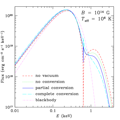
Figure 6: Spectra for hydrogen atmosphere models with $B=10^{14}$ G, $T_{\rm eff}=10^{6}$ K. The four cases described in the text are shown: (1) no vacuum (short-dashed cuve); (2) no conversion (dotted curve); (3) partial conversion (solid curve); and (4) complete conversion (long-dashed curve). The light dashed-dot curve shows the blackbody spectrum with $T=10^{6}$ K. For all three cases that include vacuum effects, the proton cyclotron feature is strongly suppressed and the high energy tail is softened relative to the no vacuum case. The “partial conversion” curve is seen to be intermediate between the “no conversion” and “complete conversion” limits.

When the vacuum polarization effect is neglected, the spectrum of a magnetic, ionized H atmosphere model generally exhibits two characteristics: (1) a hard spectral tail (compared to blackbody) due to the non-grey free-free opacity ($\kappa^{\rm ff}$ decreases with increasing photon energy; Shibanov et al., 1992; Pavlov et al., 1995); (2) a significant proton cyclotron absorption line when $E_{Bi}$ is not too far away from the blackbody peak ($\sim 3k_{B}T$) (Zane et al., 2001; Ho & Lai, 2001). Vacuum polarization tends to soften the hard spectral tail and suppress (reduce) the proton cyclotron line. These effects are discussed extensively in §4 of Ho & Lai (2003), and Lai & Ho (2003a). In Fig. 6, all of the models that include vacuum polarization effects display a large reduction in the equivalent width (EW) of the proton cyclotron feature due to the modification of the temperature profile by the vacuum resonance (see §4.1) and the mode conversion effect. The spectra also show softening of the hard spectral tail relative to the no vacuum case, though they are all still harder than blackbody. The “partial conversion” curve appears as an intermediate case between the “complete conversion” and “no conversion” extremes. The adiabatic regime where mode conversion is efficient is clearly visible: for $E\ga E_{ad}\sim 2$ keV, the “partial conversion” curve begins to follow the “complete conversion” curve.

This transition from “no conversion” to “complete conversion” is further illustrated by Fig. 7, which shows, for several photon energies $E$ (and a given direction of propagation, $\theta_{kB}$) the evolution of the specific mode intensities as a function of optical depth. At the resonance depth (denoted by the vertical lines), the X mode photons encounter the vacuum induced spike in opacity, and mode conversion occurs [governed by the non-adiabatic jump probability $P_{\rm jump}$; see eq. (4)]. As the energy is increased (from the second to bottom panels), mode conversion becomes increasingly more effective.

Figure 7: The transition from “no conversion” to “complete conversion” for a photon propagating in a hydrogen atmosphere with $B=10^{14}$ G, $T_{\rm eff}=10^{6}$ K. The top panel shows the temperature profile for this model. The bottom three panels show the evolution of the specific mode intensities for energies $E=0.35,0.65,2.72$ keV and $\theta_{kB}=\pi/4$. The dashed line shows the X-mode intensity, the solid line the O-mode intensity, and the dotted vertical lines specify the location of the vacuum resonance. For $E=0.35$ keV: $H_{\rho}=0.69$ cm, $E<E_{ad}$, and $P_{\rm jump}=1.0$, leading to minimal mode conversion. For $E=0.65$ keV: $H_{\rho}=0.78$ cm, $E\sim E_{ad}$, and $P_{\rm jump}=0.65$, leading to partial mixing of the modes. For $E=2.72$ keV: $H_{\rho}=0.98$ cm, $E>E_{ad}$, and $P_{\rm jump}=0.15$, leading to nearly complete conversion of the modes.

Figure 8 shows the spectrum for the $B=10^{14}$ G and $T_{\rm eff}=5\times 10^{6}$ K hydrogen model. All the calculations that include vacuum effects show strong suppression of the ion cyclotron feature and significant softening of the hard spectral tail. At higher effective temperatures, there is a smaller difference between the no conversion, partial conversion, and complete conversion cases. In this regime, the optical depth across the vacuum resonance is much greater than unity, and the decoupling of X-mode photons occurs at the resonance density whether or not mode conversion is taken into account (see Lai & Ho, 2002). At high energies ($E\ga 5$ keV), the models which include mode conversion are softer than those which do not.

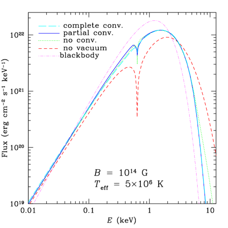
Figure 8: Same as Fig. 6, except $T_{\rm eff}=5\times 10^{6}$ K. The strength of the proton cyclotron feature is strongly suppressed for models which include vacuum polarization. At $E\ga 5$ keV, the models which include mode conversion are softer than those without, though all the atmosphere models are still harder than blackbody.

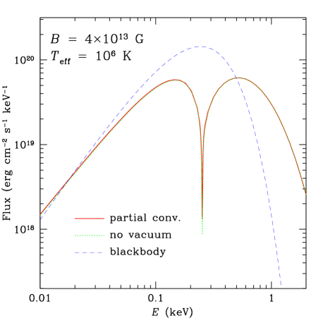
Figure 9: Spectrum of the hydrogen atmosphere model with $B=4\times 10^{13}$ G, $T_{\rm eff}=10^{6}$ K, calculated for two cases: partial mode conversion (solid curve), and no vacuum (dotted curve). The light dashed line shows the blackbody spectrum with $T=10^{6}$ K.

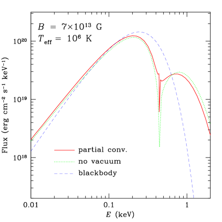
Figure 10: Same as Fig. 6, except for $B=7\times 10^{13}$ G.

Figures 9-12 depict atmosphere models at $T_{\rm eff}=10^{6}$ K with varying magnetic field strengths, comparing the “no vacuum” and correct “partial conversion” results. For $B=4\times 10^{13}$ G $<B_{l}$ (Fig. 9), the vacuum resonance lies at a lower density than the X-mode and O-mode photospheres, and vacuum polarization has a negligible effect on the spectrum, reflected by the close agreement between the “no vacuum” and “partial conversion” curves. For the hydrogen atmosphere model with $B=7\times 10^{13}$ G (Fig. 10), and the helium atmosphere model with $B=10^{14}$ G (Fig. 11), vacuum polarization affects the spectrum. For these models, $B\ga B_{l}$, and the ion cyclotron line lies near the blackbody peak. Thus, it is particularly important to treat the vacuum resonance correctly, taking partial mode conversion into account to calculate the line width. For the $B=5\times 10^{14}$ G model (Fig. 12), the spectral feature at $E_{Bi}$ is outside the energy band of observational interest. We note that at such a high field and low effective temperature, the atmosphere should contain a significant fraction of bound atoms and molecules (Ho et al., 2003; Potekhin et al., 2004), so the fully ionized model shown in Fig. 12 is not realistic.

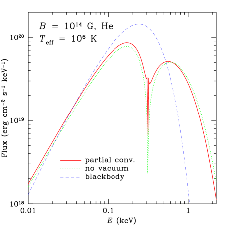
Figure 11: Same as Fig. 9, except for helium composition with $B=10^{14}$ G. The ion cyclotron line width is reduced by vacuum polarization, though it has a larger equivalent width than the model for hydrogen, due to the location of the line near the maximum of the continuum emission.

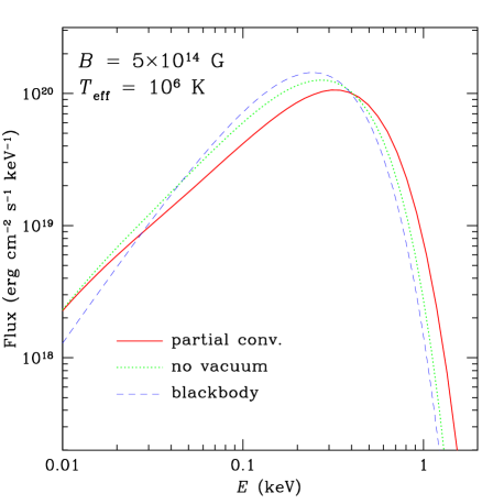
Figure 12: Same as Fig. 10, except with $B=5\times 10^{14}$ G.

Figures 13-14 show atmosphere models at magnetic field strength $B=5\times 10^{14}$ G and $T_{\rm eff}=5\times 10^{6}$ K, for hydrogen and helium compositions. At this effective temperature, the ion cyclotron feature lies close to the blackbody peak, and the effects of vacuum polarization on the line width and the spectral tail are rather pronounced.

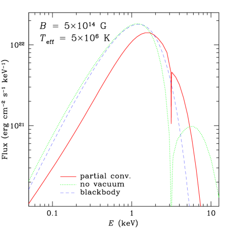
Figure 13: Same as Fig. 12, except for $T_{\rm eff}=5\times 10^{6}$ K. The proton cyclotron is strongly suppressed by vacuum polarization. The hard spectral tail is softened considerably relative to the no vacuum case, though it is still harder than blackbody.

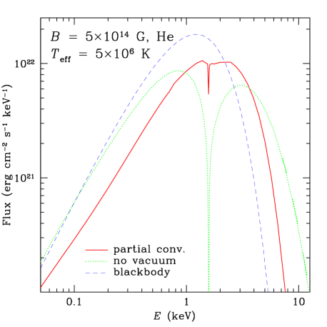
Figure 14: Same as Fig. 13, except for helium composition. Vacuum polarization strongly suppresses the ion cyclotron feature, and softens the hard spectral tail relative to the no vacuum case.

4.3 Emission beam pattern

Calculations of observed NS lightcurves and polarization signals (see §5) are critical for interpreting observations. An important ingredient of such calculations is the angular beam pattern of surface emission. Figure 15 shows the radiation intensity from a local patch of NS atmosphere (for the $T_{\rm eff}=10^{6}$ K models presented in §4.2) as a function of emission angle relative to the surface normal at several photon energies. The heavy curves show models that include vacuum polarization effects, while the lightcurves show models that neglect vacuum polarization. Magnetized atmosphere models which neglect vacuum polarization have a distinctive beaming pattern, consisting of a thin “pencil” feature at low emission angles and a broad “fan” beam at large emission angles, with a prominent gap between them (e.g., c.f., Özel, 2001). This gap tends to increase with increasing photon energy. The detailed shape of the emission beam pattern is determined by the temperature profile and the anisotropy of the mode opacities. As shown by Fig. 15, vacuum polarization tends to smooth out the gap, leading to a broad, featureless beam pattern at large magnetic fields. The broadening of the beaming pattern is due to the alteration of the temperature profile by the spike in opacity at the vacuum resonance and the mode conversion effect.

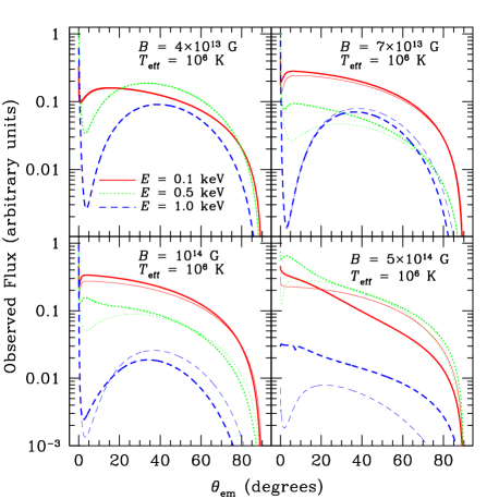
Figure 15: The specific intensity from a local patch of NS as function of emission angle $\theta_{\rm em}$ ($=\cos^{-1}\mu,$ the angle between ${\bf\hat{k}}$ and the surface normal) for hydrogen models with $T_{\rm eff}=10^{6}$ K, and $B=4\times 10^{13}$ G, $7\times 10^{13}$ G, $10^{14}$ G, $5\times 10^{14}$ G. The heavy curves show models that include vacuum polarization effects, while the lightcurves show models that neglect vacuum polarization. The latter models exhibit a characteristic beaming pattern, with a thin “pencil” shape at low emission angles and a broad “fan” at large emission angles. Inclusion of vacuum polarization tends to reduce the gap and lead to a broad, featureless beaming pattern at large magnetic fields.

Figure 16 shows the specific radiation intensity from a patch of NS atmosphere (for the $T_{\rm eff}=10^{6}$ K models presented in §4.2) at several emission angles. We see that the shape of the spectrum and EW of the absorption feature can change significantly depending on the emission angle and whether or not vacuum polarization effects are included in the calculation.

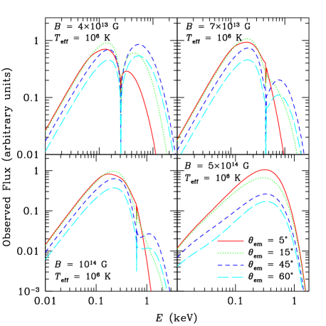
Figure 16: The specific radiation intensity from a local patch of NS atmosphere at several emission angles for hydrogen models with $T_{\rm eff}=10^{6}$ K, and $B=4\times 10^{13}$ G, $7\times 10^{13}$ G, $10^{14}$ G, and $5\times 10^{14}$ G. The shape of the spectrum and EW of the absorption feature change significantly with emission angle.

5 Polarization of the Atmosphere Emission

Thermal emission from a magnetized NS atmosphere is highly polarized. This arises from that fact that the typical X-mode photon opacity is much smaller than the O-mode opacity, $\kappa_{\rm X}\sim(E/E_{Be})^{2}\kappa_{\rm O}\ll\kappa_{\rm O}$. Thus, X-mode photons escape from deeper, hotter layers of the NS atmosphere than the O-mode photons, and the emergent radiation is linearly polarized to a high degree (as high as $100\%$) (see, e.g., Gnedin & Sunyaev, 1974; Mészáros et al., 1988; Pavlov & Zavlin, 2000)

There has been some recent interest in X-ray polarimetry for NSs (Costa et al., 2001, 2006). Observations of X-ray polarization, particularly when phase-resolved and measured in different energy bands, can provide useful constraints on the magnetic field strength and geometry, the NS rotation rate and compactness. This will be highly complimentary to the information obtained from the spectra and lightcurves. Moreover, as we show below (see also Lai & Ho 2003b), vacuum resonance gives rise to a unique polarization signature in the surface emission, even for NSs with “normal” ($B\sim 10^{12}-10^{13}$ G) magnetic fields.

Below, we calculate the observed X-ray polarizaztion signals in the case when the emission comes from a rotating magnetic hotspot on the NS surface. Although this represents the simplest situation, it captures the essential properties of the polarization signals, and the result can be carried over to more general situations. See the end of §5.3 for a discussion of the case when emission comes from an extended area (or the whole) of the stellar surface.

5.1 Geometry and lightcurves

To calculate the observed lightcurves and polarization signals, we set up a fixed coordinate system $XYZ$ with the $Z$-axis along the line-of-sight (pointing from the NS toward the observer), and the $X$-axis in the plane spanned by the $Z$-axis and ${\bf\Omega}$ (the spin angular velocity vector). The angle between ${\bf\Omega}$ and ${\bf\hat{e}}_{Z}$ is denoted by $\gamma$. The hotspot is assumed to be at the intersection of the NS surface and dipole magnetic axis, which is inclined at an angle $\eta$ relative to the spin axis. As the star rotates, the angle $\Theta$ between the magnetic axis $\mu$ and the line of sight varies according to

$$\cos\Theta=\cos\gamma\cos\eta-\sin\gamma\sin\eta\cos\psi,$$ (62)

where $\psi=(\Omega t+{\rm constant})$ is the rotation phase ($\psi=0$ when $\mu$ lies in the $XZ$ plane). We use the simplified formalism derived by Beloborodov (2002) to calculate the observed spectral flux from the area $dS$ of the hotspot, which takes the form:

$$F_{\rm obs}=\left(1-{r_{g}\over R}\right)^{3/2}I_{\nu}(\theta_{\rm em})\cos\theta_{\rm em}{dS\over D^{2}},$$ (63)

where $r_{g}=2GM/c^{2}$ is the Schwarzschild radius, $R$ is the NS radius, and $\theta_{\rm em}$ (the angle between the photon direction and the surface normal at the emission point; $\mu=\cos\theta_{\rm em}$) is related to $\Theta$ through:

$$\cos\theta_{\rm em}={r_{g}\over R}+\left(1-{r_{g}\over R}\right)\cos\Theta.$$ (64)

For $R>3r_{g}$, the spectral flux calculated using eq. (63) differs from the exact treatment (see Pechenick et al., 1983) by less than $1$%.

The top panels of Figs. 17-19 show lightcurves for NS models with several magnetic field strengths, at a range of energies $E=0.5-3$ keV, with geometry $\gamma=30\degr$, $\eta=70\degr$.

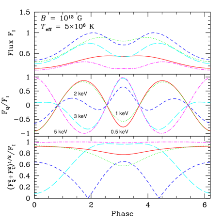
Figure 17: Lightcurve and polarization as a function of rotation phase for a NS hotspot with $B=10^{13}$ G, $T_{\rm eff}=5\times 10^{6}$ K. The angle of the spin axis relative to the line of sight is $\gamma=30\degr$, and the inclination of the magnetic axis relative to the spin axis is $\eta=70\degr$. Note that the sign of the $F_{Q}$ Stokes parameter is opposite for low and high energy photons; this implies that the planes of polarization for low and high energy photons are perpendicular. This is a unique signature of vacuum polarization for models with $B<B_{l}$.

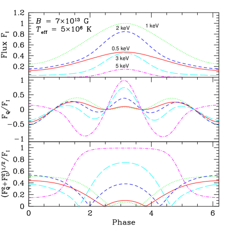
Figure 18: Same as Fig. 17 with $B=7\times 10^{13}$ G. For this model, $B\sim B_{l}$, representing the transition between the models shown in Figs. 17 and 19.

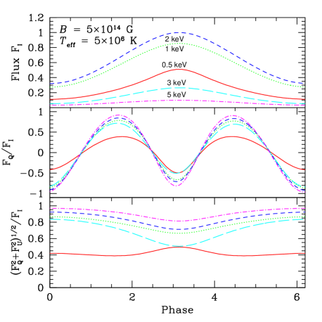
Figure 19: Same as Fig. 17 with $B=5\times 10^{14}$ G. At this field strength, $B>B_{l}$, and the vacuum resonance lies between the O and X-mode photospheres. Thus, the sign of the $F_{Q}$ Stokes parameter for low and high energy photons is the same. Note that in the top panel, the flux for the 0.5 keV case is multiplied by a factor of 10 relative to the other curves.

5.2 Observed linear polarization signals

The atmosphere models presented in §3 and §4 give the specific intensities $I_{\nu}^{\rm X}(\theta_{\rm em})$ and $I_{\nu}^{\rm O}(\theta_{\rm em})$ of the two photon modes, emerging from the NS atmosphere (outside the vacuum resonance layer). To determine the observed polarization signals, it is important to consider propagation of the polarized radiation in the NS magnetosphere. In the X-ray band, the magnetospheric dielectric properties are dominated by vacuum polarization (Heyl & Shaviv 2002). Heyl et al. (2003) (see also Heyl & Shaviv 2002) evolved the Stokes parameters along photon geodesics in the magnetosphere and showed that the observed polarization is determined at the so-called “polarization limiting radius,” at a distance far from the NS surface. Below we present a simple calculation of the propagation effect and observed linear polarization (see also Lai & Ho 2003b).

Consider a photon emitted at time $t_{i}$ from the hotspot, with rotation phase $\psi_{i}=\Omega t_{i}$. The emission point has polar angle $\Theta_{i}$ (relative to the fixed $XYZ$ frame) given by eq. (62) with $\psi=\psi_{i}$, and azimuthal angle $\varphi_{i}$ given by

$$\tan\varphi_{i}={\sin\eta\,\sin\psi_{i}\over\sin\eta\cos\gamma\cos\psi_{i}+\cos\eta\sin\gamma}.$$ (65)

This is also the angle [$\varphi_{i}=\varphi_{B}(R)$] between the projection of the magnetic axis in the $XY$ plane and the $X$-axis. After the photon leaves the star, it travels towards the observer, with a trajectory given by

$${\bf r}=(R\sin\Theta_{i}\cos\phi_{i}+\Delta_{X})\,{\hat{X}}+(R\sin\Theta_{i}\sin\phi_{i}+\Delta_{Y})\,{\hat{Y}}+(R\cos\Theta_{i}+s+\Delta_{Z})\,{\hat{Z}},$$ (66)

where $s=c\Delta t=c(t-t_{i})$, $\Delta_{X,Y,Z}$ are relativistic corrections (which, as we will see shortly, are unimportant for the polarization signals), and $\hat{X},~{}\hat{Y},~{}\hat{Z}$ are unit vectors. As the photon propagates in the magnetosphere, it will “see” a changing stellar magnetic field, given by ${\bf B}=-\nabla({\mbox{\boldmath$\mu$}}\cdot{\bf r}/r^{3})$, where

$${\mbox{\boldmath$\mu$}}=\mu\left[(\sin\eta\cos\gamma\cos\psi+\cos\eta\sin\gamma)\,{\hat{X}}+\sin\eta\sin\psi\,{\hat{Y}}+(\cos\eta\cos\gamma-\sin\eta\sin\gamma\cos\psi)\,{\hat{Z}}\right],$$ (67)

with $\psi=\Omega t=\psi_{i}+\Omega\Delta t=\psi_{i}+s/r_{l}$ (here $r_{l}=c/\Omega$ is the radius of the light cyclinder). The photon’s polarization state will evolve adiabatically following the varying magnetic field that the photon experiences, up to the polarization limiting radius $r_{\rm pl}$, beyond which the polarization is frozen. Since we anticipate $r_{\rm pl}\gg R$, we only need to consider the region far away from the NS: for $r\gg R$, the photon trajectory is simply ${\bf r}\simeq s\,{\hat{Z}}$, and the magnetic field along the photon path is ${\bf B}\simeq(2\mu_{Z}{\hat{Z}}-\mu_{X}{\hat{X}}-\mu_{Y}{\hat{Y}})/r^{3}$, with $r\simeq s$. This magnetic field has a magnitude

$$B(s)={B_{s}\over 2}\left({R\over r}\right)^{3}\left[1+3\left(\cos\eta\cos\gamma-\sin\gamma\sin\eta\cos\psi\right)^{2}\right]^{1/2},$$ (68)

where $B_{s}=2\mu/R^{3}$ is the magnitude of the (dipole) surface field at the magnetic pole. The magnetic field is inclined at an angle $\theta_{kB}$ to the line of sight, and makes an azimuthal angle $\varphi_{B}$ in the $XY$ plane such that:

$$\sin^{2}\theta_{kB}(s) = {1-\left(\cos\eta\cos\gamma-\sin\gamma\sin\eta\cos\psi\right)^{2}\over 1+3\left(\cos\eta\cos\gamma-\sin\gamma\sin\eta\cos\psi\right)^{2}},$$ (69)

$$\tan\varphi_{B}(s) = {\sin\eta\sin\psi\over\cos\eta\sin\gamma+\cos\gamma\sin\eta\cos\psi}.$$ (70)

Recall that in Eqs. (68)-(70), $\psi=\psi_{i}+s/r_{l}=\Omega t_{i}+s/r_{l}$ and $s$ is the affine parameter along the ray.

The wave equation for photon propagation in a magnetized medium takes the form

$$\nabla\times(\bar{\mbox{\boldmath$\mu$}}\cdot\nabla\times{\bf E})={\omega^{2}\over c^{2}}\mbox{\boldmath$\epsilon$}\cdot{\bf E},$$ (71)

where ${\bf E}$ is the electric field (not to be confused with the photon energy), and $\epsilon$, $\bar{\mu}$ are the dielectric and inverse permeability tensors, respectively. In the magnetized vacuum of the NS magnetosphere, they are given by $\mbox{\boldmath$\epsilon$}=a{\bf I}+q{\bf\hat{B}}{\bf\hat{B}}$ and $\mbox{\boldmath$\bar{\mu}$}=a{\bf I}+m{\bf\hat{B}}{\bf\hat{B}}$. Solving eq. (71) for EM waves with $E\propto e^{iks-i\omega t}$ yields the two modes (in the $XY$ basis)

$${\bf e}_{\rm O}=(\cos\varphi_{B},\sin\varphi_{B}),\ \ {\bf e}_{\rm X}=(-\sin\varphi_{B},\cos\varphi_{B}),$$ (72)

with indices of refraction $n_{\rm O}\simeq 1+(q/2)\sin^{2}\theta_{kB}$ and $n_{\rm X}\simeq 1-(m/2)\sin^{2}\theta_{kB}$. A general (transverse) EM wave can be written as a superposition of the two modes:

$${\bf E}={\cal A}_{\rm O}{\bf e_{\rm O}}+{\cal A}_{\rm X}{\bf e_{\rm X}}.$$ (73)

Following the steps of Lai & Ho (2002) [see their eq. (15)], we derive the following equations for the evolution of the mode amplitudes:

$$i\left(\begin{array}[]{c}{\cal A}_{\rm O}^{\prime}\\ {\cal A}_{\rm X}^{\prime}\end{array}\right) \simeq \left(\begin{array}[]{cc}-(\omega/c)\Delta n/2&i\varphi_{B}^{\prime}\\ -i\varphi_{B}^{\prime}&(\omega/c)\Delta n/2\end{array}\right)\left(\begin{array}[]{c}{\cal A}_{\rm O}\\ {\cal A}_{\rm X}\end{array}\right),$$ (80)

where the prime (’) denotes a derivative with respect to $s$, and $\Delta n=n_{\rm O}-n_{\rm X}={1\over 2}(q+m)\sin^{2}\theta_{kB}$. The condition for adiabatic evolution of photon modes is

$$(\omega/c)\Delta n\gg 2\varphi_{B}^{\prime}.$$ (81)

Near the star ($r\sim R$), $\varphi_{B}\sim 1/r$, and the adiabatic condition is easily satisfied. Far from the star ($r\gg R$), using eq. (68), we write:

$$\Delta n={\alpha\over 30\pi}\left({B\over B_{Q}}\right)^{2}\sin^{2}\theta_{kB}=9.94\times 10^{-9}B_{12}^{2}\left({R\over r}\right)^{6}F_{B},$$ (82)

where

$$F_{B}=1-\left(\cos\eta\cos\gamma-\sin\gamma\sin\eta\cos\psi\right)^{2},$$ (83)

and $B_{12}=B_{s}/(10^{12}{\rm G})$. From eq. (70), we have

$${d\varphi_{B}\over ds}={1\over r_{l}}F_{\varphi},$$ (84)

with

$$F_{\varphi}=\left(\sin^{2}\eta\cos\gamma+\sin\eta\cos\eta\sin\gamma\cos\psi\right)/F_{B}.$$ (85)

The polarization-limiting radius $r_{\rm pl}$ is set by the condition $\omega\Delta n/c=2\varphi_{B}^{\prime}$. Substituting in eqs. (82) and (84) we find

$${r_{\rm pl}\over R}=32.6\left({E_{1}B_{12}^{2}F_{B}\over f_{1}\,F_{\varphi}}\right)^{1/6},$$ (86)

where $f_{1}$ is the spin frequency $\Omega/(2\pi)$ in Hz, and $F_{B}$, $F_{\varphi}$ are slowly varying functions of phase and are of order unity. Note that the above analysis is valid only if $r_{\rm pl}\mathrel{\raise 1.29167pt\hbox{$<$}\mkern-14.0mu\lower 2.58334pt\hbox{$\sim$}}r_{l}/2$, since beyond the light-cylinder radius the magnetic field is no longer described by a static dipole. Thus we require that

$${r_{\rm pl}\over r_{l}}\simeq 6.84\times 10^{-3}\left({E_{1}B_{12}^{2}F_{B}\over F_{\varphi}}\right)^{1/6}R_{10}\,f_{1}^{5/6}\mathrel{\raise 1.29167pt\hbox{$<$}\mkern-14.0mu\lower 2.58334pt\hbox{$\sim$}}0.5,$$ (87)

where $R_{10}=R/(10~{}{\rm km})$.

Beyond $r_{\rm pl}$, the polarization state of the photon is “frozen.” Using eq. (72), the observed Stokes parameters in the observer coordinate system ($XYZ$) are given by

$$I = I_{\rm O}+I_{\rm X},$$ (88)

$$Q \simeq (I_{\rm O}-I_{\rm X})\cos 2\varphi_{B}(r_{\rm pl}),$$ (89)

$$U \simeq (I_{\rm O}-I_{\rm X})\sin 2\varphi_{B}(r_{\rm pl}),$$ (90)

where $I_{\rm O}\propto I_{\nu}^{\rm O}(\theta_{\rm em})$ and $I_{\rm X}\propto I_{\nu}^{\rm X}(\theta_{\rm em})$ are the specific mode intensities emitted at the NS surface [calculated with our models described in §3 and §4, and corrected for the general relativistic effect; see eqs. (63)-(64)], and $\varphi_{B}(r_{\rm pl})$ is evaluated at $s\simeq r=r_{\rm pl}$. From eqs. (65) and (70), with $\psi(r_{\rm pl})=\psi_{i}+r_{\rm pl}/r_{l}$, we see that the effect of NS rotation is to shift the polarization lightcurve by a phase $r_{\rm pl}/r_{l}$. For slow rotation $r_{\rm pl}/r_{l}\ll 1$ [see eq. (87)], this shift is small, and $\varphi_{B}(r_{\rm pl})\simeq\varphi_{i}+\pi$. We calculate the observed spectral fluxes $F_{I}=F,~{}F_{Q},~{}F_{U}$ associated with the intensities $I,~{}Q,~{}U$ using the standard procedure described in §5.1.

The middle and bottom panels of Figs. 17-19 show the phase evolution of the Stokes parameter $F_{Q}$ and the degree of linear polarization, both normalized to the observed spectral flux. Note that $Q$ is defined such that $Q=1$ corresponds to linear polarization in the plane spanned by the line of sight $Z$ and the NS spin axis. In Fig. 17, we consider emission from a NS hotspot with $B=10^{13}$ G and $T_{\rm eff}=5\times 10^{6}$ K. Note that the value of $F_{Q}$ for low energy photons ($E\mathrel{\raise 1.29167pt\hbox{$<$}\mkern-14.0mu\lower 2.58334pt\hbox{$\sim$}}1$ keV) is of opposite sign to that of high energy photons ($E\mathrel{\raise 1.29167pt\hbox{$>$}\mkern-14.0mu\lower 2.58334pt\hbox{$\sim$}}3$ keV). This implies that the planes of polarization for low and high energy photons are perpendicular. This is a unique signature of vacuum polarization first identified by Lai & Ho (2003b), which occurs for $B<B_{l}$ [see eq. 5] because the vacuum resonance appears outside the O-mode photosphere. Below the vacuum resonace layer ($\rho>\rho_{V}$), the X-mode flux dominates over the O-mode. For low energy photons, $E\mathrel{\raise 1.29167pt\hbox{$<$}\mkern-14.0mu\lower 2.58334pt\hbox{$\sim$}}E_{ad}$, mode conversion is inefficient, and the emergent flux is dominated by the X-mode; for high energy photons $E\mathrel{\raise 1.29167pt\hbox{$>$}\mkern-14.0mu\lower 2.58334pt\hbox{$\sim$}}E_{ad}$, mode conversion is efficient, rotating the plane of polarization, and the emergent flux is dominated by the O-mode [see Fig. 2 of Lai & Ho (2003b)].

Fig. 19 shows the same result for the model with $B=5\times 10^{14}$ G, $T_{\rm eff}=5\times 10^{6}$ K. In this case, $B>B_{l}$, the vacuum resonance appears inside the O and X-mode photospheres, and the emergent radiation is always dominated by the X-mode. As expected, the planes of polarization for low and high energy photons are aligned. Fig. 18 shows an intermediate case, where $B\sim B_{l}$ — to calculate the spectra and polarization signals for such models, it is particularly important to incorporate partial mode conversion properly. The distinct behavior between the low field and high field cases is illustrated by Fig. 20, which shows the phase-averaged $F_{Q}$ Stokes parameter as a function of photon energy for several values of the magnetic field strength. The low-field cases show the characteristic rotation of the plane of polarization between low-$E$ and high-$E$, whereas the high-field cases do not.

Figure 20: Phase average of Stokes parameter $F_{Q}$ as a function of photon energy for a rotating NS hotspot at magnetic field strengths $B=10^{13},4\times 10^{13},7\times 10^{13}$ and $5\times 10^{14}$ G, with $T_{\rm eff}=5\times 10^{6}$ K. Note that the sign of $\langle F_{Q}\rangle$ changes between low and high photon energies for the low-field cases, corresponding to rotation of the plane of polarization.

Note that in the above analysis, the observed linear polarization fraction $\Pi_{L}$ (the bottom panel of Figs. 17-19) is the same as the value just outside the emission region, $|\Pi_{em}|$, i.e.,

$$\Pi_{L}={(Q^{2}+U^{2})^{1/2}\over I}=|\Pi_{em}|,\qquad{\rm with}\quad\Pi_{em}={I_{\nu}^{O}(\theta_{em})-I_{\nu}^{X}(\theta_{em})\over I_{\nu}^{O}(\theta_{em})+I_{\nu}^{X}(\theta_{em})}.$$ (91)

The polarized fluxes are simply

$$F_{Q}\simeq F_{I}\Pi_{em}\cos 2\varphi_{B}(r_{\rm pl}),\qquad F_{U}\simeq F_{I}\Pi_{em}\sin 2\varphi_{B}(r_{\rm pl}).$$ (92)

In §5.3 we shall see that for rapidly rotating NSs, the observed $\Pi_{L}$ will be somewhat smaller than $|\Pi_{em}|$ because of the generation of circular polarization around $r_{\rm pl}$.

5.3 Circular polarization

Circular polarization of surface emission may be generated for sufficiently rapid rotating NSs due to the gradual wave mode coupling/decoupling around $r_{\rm pl}$. While the linear polarization signals can be adequately described and calculated using the simple analysis given in §5.2, to calculate the circular polarization, quantitative solutions of the evolution equations for the modes or the Stokes parameters in the magnetosphere are necessary.

Consider the mode evolution equations (80). For given initial values (e.g., mode amplitudes at $r_{i}\ll r_{\rm pl}$), the solution of the equations depend on two parameters: $C$, defined by $(\omega/c)\Delta n\approx C/r^{6}$ and $\varphi_{B}^{\prime}$ (since $\psi$ varies by a rather small amount along the ray path, $F_{B}$ and $F_{\varphi}$ are nearly constant). Alternatively, since $r_{\rm pl}$ is determined by $C/r^{6}=2\varphi_{B}^{\prime}$, the solution depends only on the dimensionless parameter $\Gamma$, defined by

$$\Gamma\equiv r_{\rm pl}\varphi_{B}^{\prime}={r_{\rm pl}\over r_{l}}\,F_{\varphi}\simeq 6.84\times 10^{-3}\left({E_{1}B_{12}^{2}F_{B}F_{\varphi}^{5}}\right)^{1/6}R_{10}\,f_{1}^{5/6}.$$ (93)

Indeed, if we define $x=r/r_{\rm pl}$, eq. (80) can be rewritten as

$$i{d\over dx}\left(\begin{array}[]{c}{\cal A}_{\rm O}\\ {\cal A}_{\rm X}\end{array}\right) \simeq \Gamma\left(\begin{array}[]{cc}-x^{-6}&i\\ -i&x^{-6}\end{array}\right)\left(\begin{array}[]{c}{\cal A}_{\rm O}\\ {\cal A}_{\rm X}\end{array}\right).$$ (100)

Note that while eq. (80) is valid for all radii, the magnetostatic approximation for the field of a rotating dipole breaks down beyond the light-cylinder radius. Since $\varphi_{B}^{\prime}\sim 1/r_{l}$, eq. (100) is valid only for $\Gamma\sim r_{\rm pl}/r_{l}\mathrel{\raise 1.29167pt\hbox{$<$}\mkern-14.0mu\lower 2.58334pt\hbox{$\sim$}}0.5$.

The Stokes parameters can be written in terms of the mode amplitudes as

$$I = |E_{X}|^{2}+|E_{Y}|^{2}=|{\cal A}_{\rm O}|^{2}+|{\cal A}_{\rm X}|^{2},$$ (101)

$$Q = |E_{X}|^{2}-|E_{Y}|^{2}=\cos 2\varphi_{B}\,(|{\cal A}_{\rm O}|^{2}-|{\cal A}_{\rm X}|^{2})-2\sin 2\varphi_{B}\,\Re e\left({\cal A}_{\rm O}{\cal A}_{\rm X}^{\ast}\right),$$ (102)

$$U = 2\,\Re e\left(E_{X}E_{Y}^{*}\right)=\sin 2\varphi_{B}\,(|{\cal A}_{\rm O}|^{2}-|{\cal A}_{\rm X}|^{2})+2\cos 2\varphi_{B}\,\Re e\left({\cal A}_{\rm O}{\cal A}_{\rm X}^{*}\right),$$ (103)

$$V = 2\,\Im m\left(E_{X}E_{Y}^{*}\right)=2\,\Im m\left({\cal A}_{\rm O}{\cal A}_{\rm X}^{*}\right).$$ (104)

Figure 21 gives some examples of the results of numerical integration of eq. (100). We start the integration at radius $x_{i}=r_{i}/r_{\rm pl}$ such that the adiabatic condition is well satisfied (we typically choose $x_{i}\mathrel{\raise 1.29167pt\hbox{$<$}\mkern-14.0mu\lower 2.58334pt\hbox{$\sim$}}1/3$). In these examples, the initial values are ${\cal A}_{\rm O}=1$, ${\cal A}_{\rm X}=0$. After obtaining ${\cal A}_{\rm O}(x)$ and ${\cal A}_{\rm X}(x)$, we calculate the Stokes parameters using eqs. (101)-(104) with $\varphi_{B}=\varphi_{B}^{\prime}(r-r_{i})=\Gamma(x-x_{i})$ (adding a constant to $\varphi_{B}$ will affect $Q$ and $U$, but not $V$). We see that for $x\mathrel{\raise 1.29167pt\hbox{$<$}\mkern-14.0mu\lower 2.58334pt\hbox{$\sim$}}1/2$, the photon modes evolve adiabatically, and thus $Q\propto\cos 2\varphi_{B}$, $U\propto\sin 2\varphi_{B}$ [see eqs.  (89)-(90)] and $V\simeq 0$. Around $x=1$ ($r=r_{\rm pl}$), the modes couple and circular polarization is generated. For $x\mathrel{\raise 1.29167pt\hbox{$>$}\mkern-14.0mu\lower 2.58334pt\hbox{$\sim$}}2$, the values of the Stokes parameters are “frozen” and no longer evolve. NSs with large $\Gamma$ (corresponding to rapid rotations; e.g., $f=40$ Hz, $B=10^{13}$ G, $E=1$ keV yields $\Gamma\sim 0.3$) can generate appreciable circular polarization, with $V(r\rightarrow\infty)/I\approx-14\%$. As the NS spin frequency decreases, the resulting $|V/I|$ decreases.

Alternatively, using the relations (101)-(104) and the mode evolution equation (80), we can derive evolution equations for the Stokes parameters:

$$I^{\prime} = 0,$$ (105)

$$Q^{\prime} = (\omega\Delta n/c)\,V\,\sin 2\varphi_{B},$$ (106)

$$U^{\prime} = -(\omega\Delta n/c)\,V\,\cos 2\varphi_{B},$$ (107)

$$V^{\prime} = -(\omega\Delta n/c)\,Q\,\sin 2\varphi_{B}+(\omega\Delta n/c)\,U\,\cos 2\varphi_{B}.$$ (108)

Since the vacuum contribution to the dielectric tensor includes no dissipation, $I^{\prime}=0$ as expected. Equations (105)-(108) can be evolved numerically to calculate the observed Stokes parameters. Again we start the integration at a radius $r_{i}<r_{\rm pl}$ such that the adiabatic condition is well satisfied. Since the circular polarization does not depend on the orientation of the $XY$ axes, we set the initial conditions at $r_{i}$ by rotating the coordinate system azimuthally so that $I=1$, $U=0$ (this also corresponds to choosing $\psi=0$ or $\varphi_{B}=0$ at $r=r_{i}$), and $Q_{i}=\Pi_{em}\leq 1$, where $\Pi_{em}$ is the linear polarization fraction just outside the atmosphere [see eq. (91)]. Since the radiation emerging from the NS surface is linearly polarized, we set $V(r_{i})=0$. Equations (105)-(108) are then integrated to a distance beyond $r_{\rm pl}$.

For a given initial value of the linear polarization fraction $\Pi_{em}$ at a small $r_{i}\ll r_{\rm pl}$, the solution of eqs. (106)-(108) depends only on the dimensionless parameter $\Gamma\equiv r_{\rm pl}\varphi_{B}^{\prime}$. Again, if we define $x=r/r_{\rm pl}$, eqs. (106)-(108) can be rewritten as

$$dQ/dx = {2\Gamma\over x^{6}}\,V\,\sin 2\varphi_{B},$$ (109)

$$dU/dx = -{2\Gamma\over x^{6}}\,V\,\cos 2\varphi_{B},$$ (110)

$$dV/dx = -{2\Gamma\over x^{6}}\left(Q\,\sin 2\varphi_{B}-U\,\cos 2\varphi_{B}\right),$$ (111)

with $\varphi_{B}=\Gamma(x-x_{i})$. We are interested in the value of $V$ at $x=x_{f}\gg 1$. Figure 21 shows some examples of the integration of Eqs. (109)-(111). Not surprisingly, the results are in exact agreement with those obtained using the mode evolution equations.

Figure 21: Evolution of the radiation mode amplitudes (top panel) and Stokes parameters (bottom three panels). The solid lines are for $\Gamma=0.3$ and the dashed lines for $\Gamma=0.1$. The polarization limiting radius is shown as the vertical dotted line. The initial values (at a small $x=x_{i}$) are ${\cal A}_{\rm O}=1,~{}{\cal A}_{\rm X}=0$, $Q=I=1,~{}U=0$ and $V=0$. At distances $x\mathrel{\raise 1.29167pt\hbox{$<$}\mkern-14.0mu\lower 2.58334pt\hbox{$\sim$}}0.5$, the modes evolve adiabatically. At $r\sim r_{\rm pl}$ the modes begin to couple, generating appreciable circular polarization. At $x\mathrel{\raise 1.29167pt\hbox{$>$}\mkern-14.0mu\lower 2.58334pt\hbox{$\sim$}}2$, the values of the Stokes parameters are “frozen”.

We have calculated the circular polarizations produced by rotating NSs with different values of $\Gamma$. Our numerical results [see Fig. (22)] show that the generated circular polarization is given by the expression

$$V/I\approx-0.60\,\Pi_{em}\,\mbox{sign}(\varphi_{B}^{\prime})\left|r_{\rm pl}\,\varphi_{B}^{\prime}\right|^{6/5}=-1.5\times 10^{-3}\,\Pi_{em}\,\left(E_{1}\,B_{12}^{2}\,F_{B}\right)^{1/5}\,f_{1}\,F_{\varphi}.$$ (112)

This expression is accurate to within one percent in the regime $\Gamma\mathrel{\raise 1.29167pt\hbox{$<$}\mkern-14.0mu\lower 2.58334pt\hbox{$\sim$}}0.4$ [see Fig. (22)]. Recall that $F_{B}\sim F_{\varphi}\sim 1$, so eq. (112) provides a quick estimate for the magnitude of the circular polarization of NS surface emission.

Figure 22: The magnitude of the observed circular polarization fraction $|V|/I$ as a function of $\Gamma$. The linear polarization fraction ($\Pi_{em}$) just outside the atmosphere is assumed to be $100\%$. The dashed line depicts the fitting formula, eq. (112), which agrees with the numerical solution to within $1\%$ for $\Gamma<0.4$. Note that solutions with $\Gamma\mathrel{\raise 1.29167pt\hbox{$>$}\mkern-14.0mu\lower 2.58334pt\hbox{$\sim$}}0.5$ are incorrect since the magnetic field around the polarization limiting radius is no longer described by the near-zone field of a rotating dipole as adopted in our calculations.

The above analysis shows that substantial circular polarization can be generated only for NSs with sufficiently rapid rotation and magnetic field strength. Given the photon energy, NS spin frequency, and dipole magnetic field strength, the degree of circular polarization from a NS can be calculated using eq. (112).

Fig. 23 shows the phase-resolved observed radiation Stokes parameters for a NS with $B=10^{13}$ G and $T_{\rm eff}=5\times 10^{6}$ K, rotating at $f=50$ Hz, with magnetic field and spin geometry $\gamma=30\degr$, $\eta=70\degr$ (this is the case shown in Fig. 17). The solid curves are numerical solutions to the Stokes parameter equations of transfer in the NS magnetosphere, while the dotted curves are calculated using the method described in § 5.2. The latter method assumes $F_{V}=0$, but yields results for $F_{Q}$ and $F_{U}$ that are quite close to those of the numerical integrations. For a rapidly rotating NS, substantial circular polarization is generated, with $|F_{V}/F_{I}|$ reaching $0.2-0.3$ in the hard X-ray band (see also Fig. 22).

Figure 23: Observed radiation Stokes parameters for a NS with $B=10^{13}$ G, $T_{\rm eff}=5\times 10^{6}$ K, $f=50$ Hz, $\gamma=30\degr$, and $\eta=70\degr$, for photon energies $E=0.5,3$ keV. The solid curves show the results of numerical integration of the transfer equations for the Stokes parameters, while the dotted curves are calculated using the approximate method of § 5.2.

Finally, we note that although the specific results presented in this section refer to emission from a hot polar cap on the NS, we expect many of our key results (e.g., rotation of the planes of linear polarization between $E\mathrel{\raise 1.29167pt\hbox{$<$}\mkern-14.0mu\lower 2.58334pt\hbox{$\sim$}}1$ keV and at $E\mathrel{\raise 1.29167pt\hbox{$>$}\mkern-14.0mu\lower 2.58334pt\hbox{$\sim$}}4$ keV due to vacuum polarization for $B\mathrel{\raise 1.29167pt\hbox{$<$}\mkern-14.0mu\lower 2.58334pt\hbox{$\sim$}}7\times 10^{13}$ G) to be valid in more complicated models (when several hotspots or the whole stellar surface contribute to the X-ray emission). This is because the polarization-limiting radius (due to vacuum polarization in the magnetosphere) lies far away from the star [see eq. 86] where rays originating from different patches of the NS experience the same dipole field (Heyl et al. 2003). Our results therefore demonstrate the unique potential of X-ray polarimetry in probing the physics under extreme conditions (strong gravity and magnetic fields) and the nature of various forms of NS.

6 Discussion

We have presented a new method for incorporating partial conversion of photon modes due to vacuum polarization into fully-ionized, self-consistent atmosphere models of magnetized NSs. This method takes into account the nontrivial probability of photon mode conversion at the vacuum resonance. While recent works have clearly identified the important effects of the vacuum resonance and related mode conversion in determining the atmosphere radiation spectrum and polarization (Lai & Ho 2003a), so far the implementation of these effects in self-consistent atmosphere models, for technical reasons, has only considered two extreme limits: complete mode conversion and no mode conversion (Ho & Lai 2003,2004). With a direct, semi-explict Runga-Kutta integration of the radiative transfer equations for the photon modes (as opposed to the forward-backward substitution procedure of the Feautrier method) and the use of an accurate mode conversion formula for each photon, our new atmosphere code displays excellent stability with respect to grid resolution. Moreover, integration of the full transfer equations for the radiation Stokes parameters shows that our treatment of partial conversion is accurate. As expected, the partial conversion solution is intermediate between the extreme cases of complete and no conversion considered previously. An accurate treatment of vacuum polarization is a critical step toward interpreting the spectra and predicting the polarization signals of magnetic NSs.

With our new atmosphere code, we have constructed a large number of atmosphere models for various magnetic field strengths, ranging from $10^{13}$ G to $5\times 10^{14}$ G, for both H and He compositions. In agreement with previous, approximate calculations (Ho & Lai 2003,2004), we find that for $B\mathrel{\raise 1.29167pt\hbox{$>$}\mkern-14.0mu\lower 2.58334pt\hbox{$\sim$}}7\times 10^{13}$ G the vacuum resonance affects the atmosphere spectra (i.e., the hard spectral tail due to nongrey opacities tends to be suppressed and the spectral line EW is reduced), and the effects become more significant as the magnetic field strength is increased. For $B\mathrel{\raise 1.29167pt\hbox{$<$}\mkern-14.0mu\lower 2.58334pt\hbox{$\sim$}}7\times 10^{13}$ G, the effect of the vacuum resonance on the spectra is smaller and becomes negligible for $B\mathrel{\raise 1.29167pt\hbox{$<$}\mkern-14.0mu\lower 2.58334pt\hbox{$\sim$}}4\times 10^{13}$ G. However, even for such “low” field strengths, vacuum resonace has a significant effect on the observed X-ray polarizations (see Lai & Ho 2003b). Our new calculations presented in this paper are particularly important for the “intermediate” field regime ($4\times 10^{13}\mathrel{\raise 1.29167pt\hbox{$<$}\mkern-14.0mu\lower 2.58334pt\hbox{$\sim$}}B\mathrel{\raise 1.29167pt\hbox{$<$}\mkern-14.0mu\lower 2.58334pt\hbox{$\sim$}}2\times 10^{14}$ G), where previous approximate treatments are inadequate. For the first time, we are able to accurately determine the $B$-dependence of the structure, spectra and polarization signals of ionized NS atmospheres.

Since the most time-consuming and difficult part of atmosphere modeling involves finding the atmosphere temperature profile that satisfies the condition of radiative equilibrium, for the convenience of the astrophysics community, we have presented fitting formulae for the temperature profiles of various atmosphere models (see §4.1). With these analytic expressions, it is relatively straightforward (using the procedure outlined in §3.1.4) to calculate various properties of the emergent radiation. These analytic profiles will also be useful for comparison with future theoretical atmosphere models.

We note that the models presented in this paper have several limitations: (1) The models assume that the magnetic field lies along the surface normal. While a more general magnetic field inclination does not change the main results of our paper (e.g. the effect of vacuum resonance and the dependence of the atmosphere spectra on $B$), to confront observations (see below), synthetic spectra must be constructed using realistic magnetic field and surface temperature distributions, adding up contributions over the entire NS surface. Such calculations are necessarily model-dependent, but they are needed for proper interpretation of observations.

(2) At high density, the radiative transfer equation breaks down, due to the dense plasma effect. At large optical depth, the photon polarization develops a non-negligible longitudinal component and the index of refraction deviates significantly from unity. This occurs when the plasma frequency of the medium exceeds the photon frequency. To date, no detailed studies of the transfer of radiation in dense plasmas have been performed, though it has been treated in an ad-hoc way by Ho et al. (2003). Nevertheless, this effect is important for treating thermal radation in the optical band, and for magnetars can affect the emission spectrum in the soft X-ray ($\mathrel{\raise 1.29167pt\hbox{$<$}\mkern-14.0mu\lower 2.58334pt\hbox{$\sim$}}1$ keV). (3) The assumption of fully ionized atmospheres may not be valid for cool NSs (such as the dim isolated NSs) or even the higher temperature AXPs and SGRs. Nevertheless, we expect features due to bound-bound and bound-free transitions of neutral species to be suppressed in the same manner as the ion cyclotron feature (see Ho et al. 2003; Potekhin et al. 2004,2005 for recent works on partially ionized magnetic atmosphere models).

6.1 Implications for observations of isolated neutron stars

As mentioned in §1, recent observations by Chandra and XMM-Newton have shown that the quiescent thermal spectra from AXPs and SGRs have no observable absorption features, such as the ion cyclotron line at $E_{Bi}=0.63(Z/A)B_{14}$ keV. As first pointed out by Ho & Lai (2003), and confirmed by our more accurate calculations presented here, the inclusion of vacuum polarization effects provides a natural explanation for the non-detection: at $B=5\times 10^{14}$ G, the vacuum-suppressed EW of the H or He cyclotron line is smaller than the current detector resolution. We expect that in the magnetar field regime, bound-bound and bound-free features will be similarly suppressed (see Ho et al. 2003; Potekhin et al. 2004).

Prominent absorption lines (at $0.7$ keV and 1.4 keV) have been detected from the source 1E1207.4-520, a young neutron star ($T\simeq 2\times 10^{6}$ K) associated with a supernova remnant (Sanwal et al., 2002; Bignami et al., 2003; De Luca et al., 2004; Mori et al., 2005) Two viable (but tentative) identifications of these features are: (1) Ion cyclotron and atomic transitions of light-element (most likely He) atmospheres at $B\mathrel{\raise 1.29167pt\hbox{$>$}\mkern-14.0mu\lower 2.58334pt\hbox{$\sim$}}10^{14}$ G (Pavlov & Bezchastnov 2005); (2) Atomic transitions of C or O atmospheres with $B\mathrel{\raise 1.29167pt\hbox{$<$}\mkern-14.0mu\lower 2.58334pt\hbox{$\sim$}}10^{12}$ G (Mori et al. 2005). Based on our general result of line suppression in the magnetar field regime, we suggest that the first interpretation is unlikely to be correct, although a quantitative calculation of the atomic line strengths is needed to draw a firm conclusion.

Absorption features have also been detected from three nearby, dim isolated NSs: RX J1308.6+2127, RX J1605.3+3249, and RX J0720.4-3125. While all three sources have similar effective temperatures ($T_{\rm eff}\sim 10^{6}$ K), their observed features occur at different energies and have varying equivalent widths: $E\approx 0.2-0.3$ keV with EW$\approx 150$ eV for RX J1308.6+2127 (Haberl et al., 2003), $E\approx 0.27$ keV with EW$\approx 40$ eV for RX J0720.4-3125 (Haberl et al., 2004a), and $E\approx 0.45$ keV with EW$\approx 80$ eV for RX J1605.3+3249 (van Kerkwijk et al., 2004). With a single line, it is difficult to conclusively determine the true atmosphere composition. One possibility is that these features are associated with proton cyclotron resonance (with possible blending from atomic transitions) in a hydrogen atmosphere (Ho & Lai 2004). For RX J1308.6+2127, the inferred magnetic field is $3-5\times 10^{13}$ G, for which line suppression by vacuum resonance is ineffective. The broad width of the feature is consistent with that calculated by our hydrogen atmosphere models (see Fig. 9). RX J1605.3+3249 is also consistent with this picture: its feature corresponds to $B\sim 7\times 10^{13}$ G, and partial suppression of the line may account for its lower (by a factor of $\sim 2$) EW (see Fig. 10). The situation for RX J0720.4-3125 is more complicated: the spectrum (including the line width) varies as a function of the rotation phase (Haberl et al. 2004a) and over a long timescale (a few years) (see Haberl et al. 2006). If its absorption feature is a proton cyclotron line, then the inferred magnetic field is too low for vacuum polarization effects to alter the line strength. Its small EW ($40$ eV) could arise if the line-emitting region (where $B\la 10^{14}$ G) is a small fraction of the NS surface; most of the surface would have $B\ga 10^{14}$ G, requiring a highly non-dipolar surface field. Alternatively, if the atmosphere of RX J0720.4-3125 is composed of helium, the required field strength is $B\sim 9\times 10^{13}$ G, strong enough for the vacuum effects to reduce the line width.

Several recent papers have identified similar absorption features in other dim isolated NSs, though these observations may require independent confirmation and/or better statistics. Haberl et al. (2004b) report spectral features for RX J0806.4-4123 ($E\approx 0.4-0.46$ keV; EW$\approx 33-56$) and RX J0420.0-5022 ($E\approx 0.3$ keV; EW$\approx 45$), while Zane et al. (2005) report a spectral feature for RX J2143.7+0654 ($E\approx 0.75$ keV; EW$\approx 27$). These features are similar to those described in more detail above, and suffer from the same difficulties of identification. Needless to say, since the magnetic field strengths of these NSs likely lie in the range $5\times 10^{13}-10^{14}$ G, for which accurate treatment of the vacuum resonance effect is crucial, the atmosphere models developed in this paper will be particularly useful, especially when combined with detailed modeling of (phase-dependent) synthetic spectra and (energy-dependent) lightcurves.

6.2 Implications for future works

It is clear that further theoretical modeling of NS surface emission is needed to confront observations. Our discussion above (§6.1) also suggests that even accurate theoretical models and high-quality data may still be inadequate to break some of the degeneracy (e.g., magnetic field strength and geomery, atmosphere composition, surface temperature distribution) inherent in the problem. In this regard, X-ray polarimetry is highly desirable. Our calculations in §5 show that polarization signals are complementary to X-ray spectra. For example, the polarization signals of magnetars and NSs with “ordinary” field strengths are qualitatively different. It is possible for a NS with a “boring” spectrum and lightcurve to generate an interesting polarization signature!

References

- Beloborodov (2002) Beloborodov, A. 2002. ApJ, 566, L85-88.
- Becker & Pavlov (2002) Becker, W., & Pavlov, G.G. 2002, in The Century of Space Science, ed. J. Bleeker et al. (Kluwer) (astro-ph/0208356)
- Bignami et al. (2003) Bignami, G., Caraveo, P., De Luca, A., Meregehetti, S. 2003. Nature, 423, 725
- Bulik & Miller (1997) Bulik, T. & Miller, M. 1997. MNRAS, 288, 596
- Burwitz et al. (2003) Burwitz, V., et al. 2003, A&A, 399, 1109
- Caraveo et al. (2004) Caraveo, P.A., et al. 2004, Science, 305, 376
- Costa et al. (2001) Costa et al. 2001. Nature, 411, 662.
- Costa et al. (2006) Costa et al. 2006. In Proc. 39th ESLAB Symposium, eds. Favata, F., Gimenez, A., SP-588, p. 141-149.
- De Luca et al. (2004) De Luca, A. Mereghetti, S., Caraveo, P., Moroni, M., Mignani, R., Bignami, G. 2004. A & A, 418, 625
- De Luca et al. (2005) De Luca, A., et al. 2005, ApJ, 623, 1051
- Drake et al. (2002) Drake, J.J. et al. 2002, ApJ, 572, 996
- Ginzburg (1964) Ginzburg, V. 1964. The Propagation of Electromagnetic Waves in Plasmas. New York: Pergamon Press.
- Gnedin & Pavlov (1974) Gnedin, Y. & Pavlov, G. 1974. Sov. Phys. JETP, 38, 903.
- Gnedin et al. (1978a) Gnedin, Yu.N., Pavlov, G.G., & Shibanov, Yu.A. 1978, Sov. Astron. Lett., 4, 117
- Gnedin & Sunyaev (1974) Gnedin, Yu. N. & Sunyaev, R.A. 1974, Astron. & Astrophys. 36, 379.
- Haberl (2005) Haber, F. 2005. in Proceedings of 2005 EPIC XMM-Newton Consortium Meeting, eds. Brield, U., Sembay, S., Read, A., 288.
- Haberl et al. (2003) Haberl et al. 2003. A & A, 403, L19.
- Haberl et al. (2004a) Haberl, F., Zavlin, V., Trümper, J., Burwitz, V. 2004. A & A, 419, 1077.
- Haberl et al. (2004b) Haberl, F., Motch, C., Zavlin, V., et al. 2004. A & A, 424, 635.
- Haberl et al. (2006) Haberl et al. 2006. A & A accepted, astro-ph/0603724.
- Heyl & Hernquist (1997b) Heyl, J. & Hernquist, L. 1997. Phys. Rev. D., 55, 2449.
- Heyl & Shaviv (2002) Heyl, J. & Shaviv, N. 2002. PhRvD, 66, 3002.
- Heyl et al. (2003) Heyl, J., Shaviv, N., Lloyd, D. 2003. MNRAS, 342, 134.
- Ho & Lai (2001) Ho, W. & Lai, D. 2001. MNRAS, 327, 1081.
- Ho & Lai (2003) Ho, W.C.G., & Lai, D. 2003, MNRAS, 338, 233
- Ho & Lai (2004) Ho, W. & Lai, D. 2004. ApJ, 607, 420.
- Ho et al. (2003) Ho, W.C.G., Lai, D., Potekhin, A.Y., Chabrier, G. 2003. ApJ, 599, 1293H.
- Ho et al. (2004) Ho, W.C.G., Lai, D., Potekhin, A.Y., Chabrier, G. 2004. AdSpR, 33, 537.
- Jackson & Halpern (2005) Jackson, M. & Halpern, J. 2005. ApJ, 633, 1114
- Jones (1986) Jones, P. 1986. MNRAS, 218, 477
- Juett et al. (2002) Juett, A.M., Marshall, H.L., Chakrabarty, D., & Schulz, N.S. 2002, ApJ, 568, L31
- Kaspi et al. (2005) Kaspi, V., Roberts, M., Harding, A. 2005. in Compact Stellar X-ray Souces, eds. Lewin, W. & van der Klis, M.
- Kulkarni et al. (2003) Kulkarni et al. 2003. ApJ, 585, 948.
- Kuiper et al. (2004) Kuiper, L, Hermsen, W., Mendez, M. 2004. ApJ, 613, 1173
- Kuiper et al. (2006) Kuiper, L., Keek, S., Hermsen, W., Jonker, P., Steeghs, D. 2006. ATel, 684
- Lai, D. (2001) Lai, D. 2001, Rev. Mod. Phys., 73, 629
- Lai & Salpeter (1997) Lai, D. and Salpeter, E.E. 1997. ApJ, 491, 270.
- Lai & Ho (2002) Lai, D., & Ho, W.C.G. 2002. ApJ, 566, 373
- Lai & Ho (2003a) Lai, D. & Ho, W. 2003. ApJ, 588, 962
- Lai & Ho (2003b) Lai, D. & Ho, W. 2003. PhRvL, 91, 1101L
- Medin & Lai (2006a) Medin, Z. and Lai, D. 2006a. Phys. Rev. A., submitted (astro-ph/0607166).
- Medin & Lai (2006b) Medin, Z. and Lai, D. 2006b. Phys. Rev. A., submitted (astro-ph/0607277).
- Mészáros & Ventura (1979) Mészáros, P. & Ventura, J. 1979, Phys. Rev. D, 19, 3565
- Mészáros et al. (1988) Mészáros, P. et al. 1988, ApJ, 324, 1056
- Mészáros (1992) Meszaros, P. 1992. High Energy Radiation from Magnetized Neutron Stars, Chicago: University of Chicago Press
- Mihalas (1978) Mihalas, D. 1978. Stellar Atmospheres, New York: W.H. Freeman and Company.
- Miller (1992) Miller, M. 1992. MNRAS, 255, 129
- Mori & Ruderman (2003) Mori, K. & Ruderman, M.A. 2003, ApJ, 592, L75
- Mori et al. (2005) Mori, K., Chonko, J.C., & Hailey, C.J. 2005, ApJ, 631, 1082
- Neuhauser et al. (1987) Neuhauser, D., Koonin, S., Langanke, K. 1987. PhRvA, 36, 4163
- Özel (2001) Özel, F. 2001. ApJ, 563, 276.
- Özel (2003) Özel, F. 2003. ApJ, 582, 31.
- Pavlov & Shibanov (1979) Pavlov, G.G. & Shibanov, Yu.A. 1979, Sov. Phys. JETP, 49, 741
- Pavlov & Zavlin (2000) Pavlov, G. & Zavlin, V. 2000. ApJ, 529, 1011
- Pavlov & Bezchastnov (2005) Pavlov, G., Bezchastnov, V. 2005. ApJ, 635, L61.
- Pavlov et al. (1995) Pavlov, G., Shibanov, Y., Zavlin, V., Meyer, R. 1995. In Alpar, M., Kiziloglu, U., van Paradijs, J., eds., Lives of the Neutron Stars. Kluwer: Boston.
- Pavlov et al. (2003) Pavlov, G.G., Sanwal, D., & Teter, M.A. 2003, in “Young Neutron Stars and Their Environments” (IAU Symp.218, ASP Conf. Proc.), eds. F. Camilo & B.M. Gaensler
- Pechenick et al. (1983) Pechenick, K., Ftaclas, C., Cohen, M. 1983. ApJ, 274, 846.
- Perez-Azorin et al. (2005) Perez-Azorin, J. et al. 2005. A&A, 433, 275
- Pons et al. (2002) Pons, J., Walter, F., Lattimer, J., Prakash, M., Neuhauser, R., An, P. 2002. ApJ, 564, 981
- Potekhin (2006) Potekhin, A. 2006. Private communication.
- Potekhin & Chabrier (2003) Potekhin, A. & Chabrier, G. 2003. ApJ, 585, 955.
- Potekhin & Chabrier (2004) Potekhin, A. & Chabrier, G. 2004. ApJ, 600, 317.
- Potekhin et al. (1999) Potekhin, A., Chabrier, G., Shibanov, Y. 1999. PhRvE, 60, 2193
- Potekhin et al. (2004) Potekhin, A., Lai, D., Chabrier, G., Ho, W. 2004. ApJ, 612, 1034
- Potekhin et al. (2005) Potekhin, A., Lai, D., Chabrier, G., Ho, W. 2005. AdSpR, 35, 1158
- Prakash et al. (2001) Prakash, M. et al. 2001, in Physics of Neutron Star Interiors, eds. D. Blaschke, N.K. Glendenning & A. Sedrakian (Springer) (astro-ph/0012136)
- Rajagopal et al. (1997) Rajagopal, M., Romani, R., Miller, M. 1997. ApJ, 479, 347
- Ruderman (1971) Ruderman, M. 1971. PhRvL, 27, 1306
- Sanwal et al. (2002) Sanwal, D., Pavlov, G., Zavlin, V., Teter, M. 2002. ApJ, 574, L61.
- Shibanov et al. (1992) Shibanov, Y, Zavlin, V., Pavlov, G., Ventura, J. 1992. A& A, 266, 313.
- Slane et al. (2002) Slane, P.O., Helfand, D.J., & Murray, S.S. 2002, ApJ, 571, L45
- Thompson & Duncan (1995) Thompson, C. & Duncan, R. 1995. MNRAS, 275, 255.
- Thompson & Duncan (1996) Thompson, C. & Duncan, R. 1996. ApJ, 473, 322.
- Tiengo et al. (2005) Tiengo, A., Mereghetti, S., Turolla, R., Zane S., Rea, N., Stella, L., Israel, G. 2005. A & A, 437, 997
- Trümper et al. (2004) Trümper, J., Burwitz, V., Haberl, F., Zavlin, V. 2004. NuPhS, 132, 560
- Turolla et al. (2004) Turolla, R., Zane, S., Drake, J. 2004. ApJ, 603, 265
- van Adelsberg et al. (2005) van Adelsberg, M., Lai, D., Potekhin, A., Arras, P. 2005. ApJ, 628, 902
- van Kerkwijk & Kulkarni (2001) van Kerkwijk, M. & Kulkarni, S. 2001. A & A, 380, 221
- van Kerkwijk et al. (2004) van Kerkwijk et al. 2004. ApJ, 608, 432.
- Ventura (1979) Ventura, J. 1979. PhRvD, 19, 1684.
- Woods & Thompson (2005) Woods, P., Thompson, C. 2005. in Compact Stellar X-ray Sources, eds. Lewin, W. & van der Klis, M.
- Yakovlev & Pethick (2004) Yakovlev, D.G., & Pethick, C.J. 2004, ARAA, 42, 169
- Zane et al. (2000) Zane, S., Turolla, R., Treves, A. 2000. ApJ, 537, 387.
- Zane et al. (2001) Zane, S., Turolla, R., Stella, L., Treves, A. 2001. ApJ, 560, 384
- Zane et al. (2005) Zane, S., Cropper, M., Turolla, R., et al. 2005. ApJ, 627, 397.
- Zavlin & Pavlov (2002) Zavlin, V. & Pavlov, G. 2002. In Proc. 270 WE-Heraeus Seminar on Neutron Stars, Pulsars and Supernova Remnants, eds. Becker, W., Lesch, H., Trümper, J., 263.