The Burst Mode of Protostellar Accretion

Abstract

We present new numerical simulations in the thin-disk approximation which characterize the burst mode of protostellar accretion. The burst mode begins upon the formation of a centrifugally balanced disk around a newly formed protostar. It is comprised of prolonged quiescent periods of low accretion rate (typically $\lesssim 10^{-7}M_{\odot}$ yr^-1) which are punctuated by intense bursts of accretion (typically $\gtrsim 10^{-4}M_{\odot}$ yr^-1, with duration $\lesssim 100$ yr) during which most of the protostellar mass is accumulated. The accretion bursts are associated with the formation of dense protostellar/protoplanetary embryos, which are later driven onto the protostar by the gravitational torques that develop in the disk. Gravitational instability in the disk, driven by continuing infall from the envelope, is shown to be an effective means of transporting angular momentum outward, and mass inward to the protostar. We show that the disk mass always remains significantly less than the central protostar mass throughout this process. The burst phenomenon is robust enough to occur for a variety of initial values of rotation rate, frozen-in (supercritical) magnetic field, and density-temperature relations. Even in cases where the bursts are nearly entirely suppressed, a moderate increase in cloud size or rotation rate can lead to vigorous burst activity. We conclude that most (if not all) protostars undergo a burst mode of evolution during their early accretion history, as inferred empirically from observations of FU Orionis variables.

1 Introduction

Many stars in the pre-main sequence evolutionary stage are known to vary in brightness. For instance, T Tauri and Herbig Ae/Be stars change in brightness by about one magnitude in irregular intervals and EXors show short-lasting variations of 1-3 magnitudes. However, the stars with the largest amplitude brightness variations (3-6 magnitudes during $\leq 100$ yr) are the FU Ori stars named after the prototype FU Orionis (Herbig, 1977). A sharp increase in the mass accretion rate onto a protostar is widely thought to be responsible for the FU Ori outbursts.

Several possible physical mechanisms for elevated mass accretion rates in young stars have been proposed. For instance, a strong dependence of the effective viscosity on the gas temperature in the innermost regions of a circumstellar disk can cause a temporary increase in the viscous mass transfer rate and generate mass accretion bursts (Lin & Papaloizou, 1985; Clarke et al., 1990). The thermal instability theory has been refined to successfully model the duration and inferred repetition timescale of FU Ori outbursts, and even to model individual light curves of a few objects (Bell & Lin, 1994; Bell et al., 1995). Nevertheless, these models depend upon the ad hoc $\alpha$ viscosity prescription (Shakura & Sunyaev, 1973), which parametrizes the physical mechanism of angular momentum transport. Another possible cause of FU Ori outbursts is a close encounter of protostars in a binary system, resulting in tidal effects in the disks and mass transfer (Bonnell & Bastien, 1992). This mechanism obviously fails to explain the FU Ori phenomenon in isolated protostars.

In recent years, a new mechanism for the generation of FU Ori eruptions has begun to emerge. Theoretical and numerical studies of protostellar disks show that they are subject to gravitational instabilities which redistribute the mass and angular momentum in the disk (Tomley et al., 1994; Laughlin & Bodenheimer, 1994). Boss (2003) has found that the gravitational instability in marginally unstable disks can lead not only to a steady inward mass transport but also to protoplanet formation. Mejía et al. (2005) have reported three-dimensional disk simulations that demonstrate a single FU-Ori-like mass accretion burst related to the growth of spiral instability. The above-mentioned models all study the evolution of an isolated protostellar or protoplanetary disk. In our recent paper (Vorobyov & Basu, 2005c, hereafter Paper I) we presented the first model of cloud core collapse which generates episodic mass accretion and luminosity bursts that can be identified with FU Ori eruptions. The disk that forms self-consistently in our model from the collapse of a cloud core is necessarily not isolated from its parent cloud core envelope. The results presented in Paper I showed that the infall of matter from the surrounding envelope can periodically destabilize the disk and lead to the formation of spiral structure and dense clumps within the arms. Gravitational torques associated with the spiral arms drive the clumps onto the protostar, generating mass accretion amd luminosity bursts comparable to those observed in FU Ori stars. This process repeats until most of the envelope has been accreted onto the protostellar disk. We note that this process bears a remarkable resemblance to the empirically inferred history of disk accretion advocated by Kenyon et al. (1990), and reviewed by e.g., Hartmann & Kenyon (1996).

We refer to the newly discovered mode of protostellar accretion as the “burst mode”. It follows an earlier “smooth mode” of accretion that is characteristic of mass accretion onto the protostar before a disk has formed. The smooth mode accretion rate may continue to be used as a value for envelope accretion onto the disk after its formation. The smooth mode accretion has been extensively studied in the literature, accounting for the influence of various initial conditions and physical processes. In the prototypical model of smooth mode accretion (Shu, 1977), the accretion rate is proportional to $c_{\rm s}^{3}/G$, where $c_{\rm s}$ is the isothermal sound speed and $G$ is the gravitational constant. The proportionality constant is 0.975 in the case of a static equilibrium singular isothermal sphere (SIS) density profile ($\rho=c_{\rm s}^{2}/2\pi Gr^{2}$) at the moment of protostar formation ($t=0$). However, it is increasingly greater for profiles that are overdense compared to the SIS but still proportional to $r^{-2}$. The effect of nonzero but spatially uniform velocities at $t=0$ is to increase the accretion rate further (Hunter, 1977; Fatuzzo et al., 2004), while remaining proportional to $c_{\rm s}^{3}/G$. The effect of spatially nonuniform velocities that are commonly generated in models of prestellar collapse is to introduce a time dependence into the accretion rate. There is an initially high accretion rate that is reminiscent of the self-similar solution derived by Hunter (1977) – due to an inner region of supersonic infall at $t=0$ – but a subsequent decline and later accretion rate that is closer to the Shu rate (Hunter, 1977; Foster & Chevalier, 1993). The effect of magnetic fields is to increase the constant accretion rate somewhat in the case of static initial conditions (Li & Shu, 1997) and to increase the time-dependent accretion rate for nonzero and spatially nonuniform infall at $t=0$ (Tomisaka, 1996; Ciolek & Königl, 1998). A finite mass reservoir will clearly introduce a final phase of terminally declining accretion rate. Therefore, the smooth mode accretion can be conceptually divided into three phases (Vorobyov & Basu, 2005a, b): an early phase of high but declining accretion rate, an intermediate phase of steady accretion at a rate proportional to $c_{\rm s}^{3}/G$ (this phase may not exist if the cloud core is sufficiently small), and a final phase of terminally declining accretion rate.

In the present paper, we investigate further the effect of rotation and nonaxisymmetry in generating the burst mode of accretion. For better study of the influence of rotation and comparison with spherically symmetric models, we also present nonrotating models. Furthermore, we investigate the role of frozen-in magnetic fields and thermal evolution in determining the frequency and amplitude of mass accretion bursts. We show how the burst mode of protostellar accretion is related to the three phases of smooth mass accretion, since the latter still characterize the infall onto a protostellar disk after its formation.

The basic equations that we solve and the numerical techniques are described in § 2, while the results of our simulations are presented in § 3. Further discussion is given in § 4 and the results are summarized in § 5. The Appendix describes some tests of our numerical code.

2 Formulation of the Problem

2.1 Basic Equations

We consider cloud cores that have dynamically decoupled from a diffuse parent cloud, and which are flattened due to the influence of an energetically significant large-scale magnetic field and/or rotation. We use the magnetized thin-disk approximation (Ciolek & Mouschovias, 1993; Basu & Mouschovias, 1994) generalized to nonaxisymmetric form. The thin-disk approximation is justified certainly during the prestellar collapse phase, as the core quickly establishes near force-balance along the mean magnetic field direction (Fiedler & Mouschovias, 1993). We also assume a spatially uniform mass-to-flux ratio, which is approximately valid for much of the supercritical phase of collapse (Basu, 1997).

The basic model is as follows. In the vertical ($z$) direction coinciding with the mean magnetic field, we use a one-zone approximation, so that the cloud of half thickness $Z(r,\phi,t)$ contains a vertically uniform density $\rho(r,\phi,t)$ and vertically uniform magnetic field $B_{z}(r,\phi,t)\mbox{\boldmath$\hat{z}$}$, where $r$ and $\phi$ are the radial and azimuthal coordinates in the disk equatorial plane, and $t$ is the time. The magnetic field has nonzero components in all three directions above the disk surface. In particular, at the top ($z=Z$) and bottom ($z=-Z$) surfaces of the cloud, the magnetic field is

$$\mbox{\boldmath$B$}(r,\phi,z=Z,t) = B_{z}^{+}\mbox{\boldmath$\hat{z}$}+B_{r}^{+}\mbox{\boldmath$\hat{r}$}+B_{\phi}^{+}\mbox{\boldmath$\hat{\phi}$},$$ (1)

$$\mbox{\boldmath$B$}(r,\phi,z=-Z,t) = B_{z}^{-}\mbox{\boldmath$\hat{z}$}+B_{r}^{-}\mbox{\boldmath$\hat{r}$}+B_{\phi}^{-}\mbox{\boldmath$\hat{\phi}$}.$$ (2)

The physical variables on the right hand side of the above equations are functions of $(r,\phi,t)$; all thin-disk variables subsequently listed will be assumed to carry this dependence. To simplify further, we note that reflection symmetry about the midplane implies that $B_{z}^{-}=B_{z}^{+}$, $B_{r}^{-}=-B_{r}^{+}$, and $B_{\phi}^{-}=-B_{\phi}^{+}$. We shall also assume that the vertical component of the magnetic field inside the disk equals that just outside, i.e., $B_{z}^{+}=B_{z}$; this actually ignores a correction term proportional to $\nabla_{p}Z$ (Ciolek & Mouschovias, 1993), where $\nabla_{p}=\mbox{\boldmath$\hat{r}$}\partial/\partial r+\mbox{\boldmath$\hat{\phi}$}\,r^{-1}\partial/\partial\phi$ is the gradient along the planar coordinates of the disk. Terms that are proportional to $\nabla_{p}Z\sim Z/r$ amount to small corrections to the thin disk equations, and are generally dropped for simplicity in this study. For ease of notation, we subsequently drop all $+$ superscripts for magnetic field components at the disk surface.

Integration of the ideal MHD equations in the $z-$direction, from $z=-Z(r,\phi,t)$ to $z=Z(r,\phi,t)$ and use of Leibnitz’s Rule for Differentiation of Integrals and the Fundamental Theorem of Calculus, yields the following equations for mass and momentum transport:

$$\frac{{\partial\Sigma}}{{\partial t}} = -\nabla_{p}\cdot\left(\Sigma\mbox{\boldmath$v$}_{p}\right),$$ (3)

$$\Sigma\frac{d\mbox{\boldmath$v$}_{p}}{dt} = -\nabla_{p}{\cal P}-\frac{Z}{{4\pi}}\nabla_{p}B_{z}^{2}+\frac{{B_{z}\mbox{\boldmath$B$}_{p}}}{{2\pi}}+\Sigma\mbox{\boldmath$g$}_{p}\,.$$ (4)

In the above equations, $\Sigma$ is the mass surface density of the disk, ${\cal P}\equiv\int_{-Z}^{Z}Pdz$ is the vertically integrated form of the gas pressure $P$, $\mbox{\boldmath$v$}_{p}=v_{r}\mbox{\boldmath$\hat{r}$}+v_{\phi}\mbox{\boldmath$\hat{\phi}$}$ is the velocity in the disk plane, $\mbox{\boldmath$B$}_{p}=B_{r}\mbox{\boldmath$\hat{r}$}+B_{\phi}\mbox{\boldmath$\hat{\phi}$}$ is the planar magnetic field at the top surface of the disk, and $\mbox{\boldmath$g$}_{p}=g_{r}\mbox{\boldmath$\hat{r}$}+g_{\phi}\mbox{\boldmath$\hat{\phi}$}$ is the gravitational field in the disk plane. Both $\mbox{\boldmath$v$}_{p}$ and $\mbox{\boldmath$g$}_{p}$ are assumed to be $z-$independent for simplicity. In this derivation, we have neglected the effect of an external bounding pressure on the cloud, and dropped all terms proportional to $\nabla_{p}Z$ in the integrated magnetic force. Note the formal similarity between the magnetic pressure ($-2Z\nabla_{p}B_{z}^{2}/8\pi$) and thermal pressure ($-\nabla_{p}{\cal P}\simeq-2Z\nabla_{p}P$) terms, as well as between the magnetic tension ($B_{z}\mbox{\boldmath$B$}_{p}/2\pi$) and gravity ($-g_{z}\mbox{\boldmath$g$}_{p}/2\pi G$) terms for a thin sheet, in which $g_{z}=-2\pi G\Sigma$.

In order to calculate the forces due to gas pressure and magnetic pressure, we have to specify the half-thickness $Z$ in the effectively optically thin (isothermal) and optically thick (nonisothermal) regimes. During the isothermal phase of evolution, local vertical hydrostatic equilibrium (ignoring external gas and magnetic field pressure) implies that

$$\rho c^{2}_{\rm s}=\frac{\pi}{2}G\Sigma^{2},$$ (5)

where $c_{\rm s}$ is the isothermal sound speed. This relation allows a straightforward determination of the half-thickness $Z\equiv\Sigma/2\rho$. For the optically thick regime, we make use of the radiation hydrodynamic simulations of spherical cloud collapse by Masunaga et al. (1998), who have shown that the size of the central optically thick region stays constant at approximately 5 AU and is independent of the mass of a parent cloud and of the initial density distribution. Therefore, we seek to capture the essential physics of both regimes by letting

$$Z=\left\{\begin{array}[]{ll}c^{2}_{\rm s}/\pi G\Sigma&{\rm if}\>\>\Sigma<\Sigma_{\rm cr},\\ c^{2}_{\rm s}/\pi G\Sigma_{\rm cr}&{\rm if}\>\>\Sigma\geq\Sigma_{\rm cr}.\end{array}\right.$$ (6)

We set the critical surface density $\Sigma_{\rm cr}=36.2$ g cm^-2, which corresponds to the critical gas volume density $n_{\rm cr}=10^{11}$ cm^-3 (Larson, 2003) for a gas disk in vertical hydrostatic equilibrium at $T=10$ K. The dependence of our results on the adopted value of $\Sigma_{\rm cr}$ is discussed in § 3.4.

We assume isothermal evolution up to some critical density, and a polytropic pressure-density relation for the later optically thick regime. This assumption, along with the adopted half-thickness $Z$ of the thin-disk, can be used to derive the following simplified expression for the integrated gas pressure as a function of surface density:

$${\cal P}=c_{\rm s}^{2}\Sigma+c_{\rm s}^{2}\Sigma_{\rm cr}\left(\Sigma\over\Sigma_{\rm cr}\right)^{\gamma}.$$ (7)

Equation (7) allows for a smooth transition between the isothermal and nonisothermal regimes. The gas temperature can be determined via the ideal gas equation of state ${\cal P}=\Sigma kT/m$, so that

$$T={c^{2}_{\rm s}m\over k}\left[1+\left(\Sigma\over\Sigma_{\rm cr}\right)^{\gamma-1}\right],$$ (8)

where $k$ is Boltzmann’s constant and $m$ is the mean molecular mass. We adopt the ratio of specific heats $\gamma=7/5$ for the optically thick regime, appropriate for an adiabatic diatomic gas. If the temperature is low, neither rotational nor vibrational modes of molecular hydrogen are excited. In this case, the ratio of specific heats is $\gamma=5/3$. We explore the dependence of our results on the adopted value of $\gamma$ in § 3.4.

The gravitational field $\mbox{\boldmath$g$}(r,\phi,z,t)=-\nabla\Phi(r,\phi,z,t)$, where $\Phi$ is the scalar gravitational potential. If the material outside the thin disk is assumed to contain negligible mass, then $\Phi$ is formally the solution of Laplace’s equation

$$\nabla^{2}\Phi=0$$ (9)

above the disk. For this purpose, we work in the limit $Z\rightarrow 0$, in which case the solution is subject to the boundary conditions

$$\frac{\partial\Phi}{\partial z}=2\pi G\Sigma\>(z=0),\>\>\Phi\rightarrow 0\>(z\rightarrow\infty).$$ (10)

The gravitational field in the plane of the thin sheet is

$$\mbox{\boldmath$g$}_{p}(r,\phi,t)=-\nabla_{p}\Phi(r,\phi,z=0,t).$$ (11)

The solution for the potential in the plane of the nonaxisymmetric sheet is

$$\Phi(r,\phi,z=0,t) = -G\int_{0}^{r_{\rm out}}r^{\prime}dr^{\prime}$$ (12)

$$\times\int_{0}^{2\pi}\frac{\Sigma(r^{\prime},\phi^{\prime})d\phi^{\prime}}{\sqrt{{r^{\prime}}^{2}+r^{2}-2rr^{\prime}\cos(\phi^{\prime}-\phi)}}\,,$$

where $r_{\rm out}$ is the size of the cloud core (see Binney & Tremaine, 1987).

Due to our assumption of flux-freezing and a spatially uniform mass-to-flux ratio, the vertical magnetic field component in the disk is easily determined by the relation

$$B_{z}=\alpha\,2\pi G^{1/2}\Sigma,$$ (13)

where $\mu\equiv\alpha^{-1}$ is the mass-to-flux ratio in units of the critical value for collapse $(2\pi G^{1/2})^{-1}$ for a thin sheet (Nakano & Nakamura, 1978). We note that during the isothermal phase of evolution, both the gas pressure and magnetic pressure gradient terms can be simplified so that their sum equals $(1+2\alpha^{2})c^{2}_{\rm s}\nabla_{p}\Sigma$ (Basu, 1997; Shu & Li, 1997; Nakamura & Hanawa, 1997).

If we assume that the material above the thin disk (already assumed to carry negligible inertia) is also current-free ($\nabla\times\mbox{\boldmath$B$}=0$), then the magnetic field above the disk satisfies $\mbox{\boldmath$B$}(r,\phi,z,t)=\nabla{\Psi}(r,\phi,z,t)$, where $\Psi$ is a scalar magnetic potential. The condition $\nabla\cdot\mbox{\boldmath$B$}=0$ means that we can determine $\Psi$ by solving

$$\nabla^{2}\Psi=0,$$ (14)

subject to the boundary conditions (in the limit $Z\rightarrow 0$)

$$\frac{\partial\Psi}{\partial z}=B_{z}\>(z=0),\>\>\Psi\rightarrow 0\>(z\rightarrow\infty).$$ (15)

Once a solution is obtained, we calculate

$$\mbox{\boldmath$B$}_{p}(r,\phi,t)=\nabla_{p}\Psi(r,\phi,z=0,t).$$ (16)

Equations (9)-(11) and (14)-(16) show that there is a formal similarity in how $\mbox{\boldmath$B$}_{p}$ is determined from $B_{z}$ and $\mbox{\boldmath$g$}_{p}$ is determined from $g_{z}(=-2\pi G\Sigma)$. The symmetry is even stronger due to our assumption of uniform mass-to-flux ratio (eq. [13]), so that

$$\mbox{\boldmath$B$}_{p}=-\frac{\alpha}{G^{1/2}}\mbox{\boldmath$g$}_{p}\Rightarrow\frac{B_{z}\mbox{\boldmath$B$}_{p}}{2\pi}=-\alpha^{2}\mbox{\boldmath$g$}_{p}.$$ (17)

Altogether, equations (3)-(4), (6)-(7), (11)-(13), and (17) form a closed system of equations for the evolution of the thin disk.

2.2 Numerical Methods

The thin-disk equations are solved numerically in polar coordinates ($r,\phi$) using the method of finite differences with a time-explicit, operator split solution procedure similar to that described by Stone & Norman (1992) for their ZEUS-2D code. Advection is performed using the second-order van Leer (1977) scheme. The timestep is determined according to the usual Courant-Friedrichs-Lewy criterion. The numerical grid has $128\times 128$ points, which are uniformly spaced in the azimuthal direction and logarithmically spaced in the $r$-direction, i.e., the radial grid points are chosen to lie between the inner boundary $r_{\rm in}$ and outer boundary $r_{\rm out}$ so that they are uniformly spaced in $u=\log r$. With 128 radial points, the innermost cell size is 0.56 AU for our typical adopted values $r_{\rm in}=10$ AU and $r_{\rm out}=10^{4}$ AU. We introduce a “sink cell” at $r<r_{\rm in}=10$ AU, which represents the central protostar plus some circumstellar disk material, and impose a free inflow inner boundary condition. We trace the value of the gas surface density in the sink cell and we assume the formation of a central protostar when it exceeds the critical density $\Sigma_{\rm cr}$. The gas that passes through the sink cell is then distributed in a $90\%:10\%$ proportion between the protostar (the central point object) and the inner circumstellar disk. The main results are insensitive to the details of mass distribution in the sink cell. We assume that the matter is cycled through the inner circumstellar disk and onto the protostar rapidly enough so that the mass infall through the sink cell is at least proportional to the mass accretion rate onto the protostar.

In our models, the gravitational potential $\Phi$ consists of three parts: a central protostar, an inner circumstellar disk, and the cloud core. The gravitational potential of the protostar is that of a point mass. The gravitational potential of the inner circumstellar disk ($0~{}{\rm AU}<r<10$ AU) is computed by decomposing it into a series of twenty concentric circular rings of constant density and summing the input from each ring. The gravitational potential of an $i$-th ring in the plane of the ring is computed using a power series expansion in $r$:

$$\Phi_{i}(r)=-{GM_{i}\over r}\left(1+{a_{i}^{2}\over 4r^{2}}+{a_{i}^{4}\over 16r^{4}}+\ldots\right)\,\,(r>a_{i}),$$ (18)

where $a_{i}$ is the radius of an $i$-th ring and $M_{i}$ is its mass. The potential due to the extended mass distribution of the cloud core (i.e., all the material outside the sink cell) is calculated as described in Binney & Tremaine (1987, p. 96). A change of variables and use of a numerical grid that is logarithmically spaced in the $r$-direction allows us to reduce the integral in equation (12) to a sum that can be evaluated by a Fast Fourier Transform technique.

The results of some relevant numerical test problems are presented in the Appendix.

2.3 Initial and boundary conditions

Our model cloud cores are composed of molecular hydrogen with a $10\%$ admixture of atomic helium (so that $m=2.33\,m_{\rm H}$, where $m_{\rm H}$ is the atomic hydrogen mass) and are initially isothermal with $T=10$ K ($c_{\rm s}=0.188$ km s^-1). The initial surface density and angular velocity distributions of cloud cores are based on the analytic best-fits to numerical models of collapsing magnetically supercritical cores (Basu, 1997):

$$\Sigma={r_{0}\Sigma_{0}\over\sqrt{r^{2}+r_{0}^{2}}},$$ (19)

$$\Omega=2\Omega_{0}\left({r_{0}\over r}\right)^{2}\left[\sqrt{1+\left({r\over r_{0}}\right)^{2}}-1\right].$$ (20)

Here, $\Sigma_{0}$ and $\Omega_{0}$ are the central surface density and angular velocity, respectively. The above profiles have the property that the specific angular momentum $K=\Omega\,r^{2}$ is a linear function of the enclosed mass $M$. We choose a value $r_{0}=\sqrt{2}c_{\rm s}^{2}/(\pi G\Sigma_{0})$, so that $r_{0}$ is comparable to the Jeans length of an isothermal sheet. More specifically, we note that the gravitational field of a thin disk with the surface density (19) is

$$g_{r}=\frac{-2\pi G\Sigma_{0}r}{(r^{2}+r_{0}^{2})^{1/2}[1+(1+r^{2}/r_{0}^{2})^{1/2}]}\>.$$ (21)

For small radii, the ratio of thermal pressure acceleration to gravity is $a_{\rm T}/|g_{r}|=c_{\rm s}^{2}/\pi G\Sigma_{0}r_{0}$, and is equal to 0.707 for the choice of $r_{0}$ above. The ratio $a_{\rm T}/|g_{r}|$ is half this value in the large radius limit.

We introduce a weak nonaxisymmetric perturbation into the initially axisymmetric density distribution by substituting $r^{2}$ in equation (19) with $r^{2}({\cos^{2}\phi/a^{2}}+a^{2}\sin^{2}\phi)$. The parameter $a=0.98$ denotes the cloud oblateness. Rotation and magnetic fields are introduced in some models through the parameters $\Omega_{0}$ and $\alpha$. They are chosen so that the cores are initially gravitationally unstable, i.e., the ratio of the sum of rotational, magnetic, and thermal energies to the magnitude of gravitational energy is less than unity. We emphasize that our qualitative results are insensitive to the particular choice of initial surface density and angular velocity distributions.

We impose an outer boundary condition such that the gravitationally bound cloud core has a constant mass and volume. The assumption of a constant mass is observationally justified by the detection of sharp boundary edges in the radial gas density distribution of pre-stellar cloud cores (Ward-Thompson et al., 1999; Bacmann et al., 2000). Physically, this assumption is justified if the cloud core can dynamically decouple from the parent diffuse cloud due to a much shorter dynamical timescale in the contracting central condensation than in the external region. A specific example of such a decoupling is the ambipolar-diffusion induced core formation in magnetically supported clouds (e.g., Basu & Mouschovias, 1995b). The assumption of a constant volume implies a constant radius of gravitational influence of a cloud core within a parent diffuse cloud.

3 Results

3.1 Mass accretion rate in nonrotating cloud cores

The behavior of the mass accretion rate onto the protostar plus circumstellar disk system in spherical finite-mass models was analytically and numerically studied by Henriksen et al. (1997), Whitworth & Ward-Thompson (2001), and Vorobyov & Basu (2005a). They showed the importance of a finite mass reservoir as the cause of an ultimately declining mass accretion rate, an effect that is necessarily not part of a self-similar solution like that of Shu (1977). In particular, Vorobyov & Basu (2005a) argued that a finite mass reservoir and an associated phase of declining mass accretion rate and declining bolometric luminosity is necessary to understand the Class I evolutionary phase of protostars.

In this section, we present a prototype cloud core (hereafter, model 1) with outer radius $r_{\rm out}=10^{4}$ AU and mass $M_{\rm c}=1.0~{}M_{\odot}$. It is nonrotating ($\Omega_{0}=0$) and nonmagnetic ($\alpha=0$). The parameters of this and other models are listed in Table 1. All model cloud cores have $\Sigma_{0}=0.12$ g cm^-2 (corresponding to a central number density $n_{0}=10^{6}$ cm^-3), but differ in the values of other parameters ($\Omega_{0},~{}\alpha,~{}\gamma$, etc.).

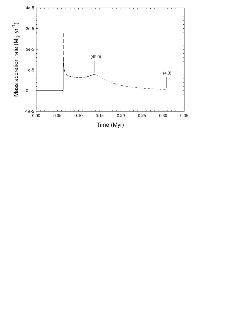
Figure 1: Temporal evolution of the mass accretion rate $\dot{M}$ in the nonrotating and nonmagnetized model 1. Three distinct phases in $\dot{M}$ are shown by the dash-dotted, dashed, and dotted lines (see explanation in the text). The numbers in parentheses indicate the percentage of the total cloud core mass left in the envelope at the corresponding evolutionary time.

We compute the mass accretion rate $\dot{M}=-2\pi r\Sigma v_{r}$ after protostar formation at $r=r_{\rm in}=10$ AU in model 1, and compare the results with that obtained in spherical collapse models by Vorobyov & Basu (2005a). Figure 1 shows the temporal evolution of $\dot{M}$, which is characterized by three distinct phases after protostar formation at $t=0.064$ Myr. In the early phase, shown in Figure 1 by the dash-dotted line, $\dot{M}$ is declining due to a gradient of infall velocity in the inner region, which is an effect not predicted by isothermal similarity solutions. In the intermediate phase that follows the initial decline in $\dot{M}$ and is shown in Figure 1 by the dashed line, $\dot{M}$ attains a near constant value ($\propto c_{\rm s}^{3}/G$) which is consistent with the standard theory of Shu (1977). The later phase of mass accretion, shown in Figure 1 by the dotted line, is a result of the finite mass reservoir in our model. A shortage of matter developing at the outer edge of a core generates an inward-propagating rarefaction wave that steepens the radial gas density profile. When accretion occurs from the mass shells in the region affected by the rarefaction wave at the time of protostar formation, a rapid and terminal decline in $\dot{M}$ occurs. These three phases, calculated in disklike geometry, confirm the general picture described by Vorobyov & Basu (2005a) for spherical hydrodynamic collapse. However, unlike the spherically symmetric model, there is a small rise in $\dot{M}$ between the intermediate and late phases of mass accretion. This effect is due to the flattened geometry of the cloud core. The gravitational field at the edge of a truncated flattened core is greater in magnitude than the corresponding field in an infinite cloud with a low density tail. This is due to the fact that the net gravitational field acting on any mass shell is a sum of contributions from both the inner and outer mass shells, unlike in spherical geometry. The missing effect of an outward pull from mass that would be located outside the cloud boundary makes the net (inward) gravity increase in magnitude near the cloud boundary rather than continue the expected monotonic decline. The extra inward pull on these mass shells leads to the small rise in $\dot{M}$ during the latter part of the intermediate phase. This effect is accentuated in our model by the use of the infinitesimally-thin-disk approximation for calculating the gravitational field.

Hereafter, we refer to the three phases of accretion as the early-decline (or early) accretion phase, the intermediate-near-constant (or intermediate) accretion phase, and the terminal-decline (or terminal) accretion phase. We find that sufficiently extended cloud cores show all three phases while more compact cores usually do not experience the intermediate phase. For example, the cloud core in model 1 has $r_{\rm out}/r_{0}\approx 7$, and is sufficiently large to exhibit a well developed intermediate accretion phase. This result is qualitatively consistent with our earlier results in spherical geometry (Vorobyov & Basu, 2005a).

3.2 Mass accretion rate in rotating cloud cores

In Paper I, we demonstrated through high-resolution simulations in the thin-disk approximation that the collapse of a rotating cloud core and self-consistent formation of a protostellar disk leads to a burst mode of protostellar accretion. The earlier smooth mode of accretion is reminiscent of the collapse of a spherical cloud (Vorobyov & Basu, 2005a) or a nonrotating disklike cloud as presented in the previous section. The later burst mode starts when the protostellar disk forms around the protostar. In this mode, the mass accretion is distinguished by very short but vigorous accretion bursts, which are interspersed within longer periods of quiescent low-rate accretion.

In this section, we investigate the role of rotation in determining the amplitude and frequency of mass accretion bursts and implied observable quantities. We also demonstrate how the two modes of accretion in rotating cloud cores are linked with the three phases of mass accretion in nonrotating cloud cores. The rotational and gravitational energies of the initial (axisymmetric) cloud core are calculated here as

$$E_{\rm rot}=2\pi\int\limits_{r_{\rm in}}^{r_{\rm out}}ra_{\rm c}\Sigma\,r\,dr,$$ (22)

$$E_{\rm grav}=-2\pi\int\limits_{r_{\rm in}}^{\rm r_{\rm out}}rg_{r}\Sigma\,r\,dr,$$ (23)

respectively, where $a_{\rm c}=\Omega^{2}r$ is the centrifugal acceleration.

We study in detail a cloud core that has the same parameters as model 1 but also rotates according to equation (20). This cloud core (hereafter, model 2) has a central angular velocity $\Omega_{0}=1.5$ km s^-1 pc${}^{-1}=4.86\times 10^{-14}$ rad s^-1, leading to a ratio of centrifugal acceleration to gravity $a_{\rm c}/|g_{r}|=\Omega_{0}^{2}r_{0}/\pi G\Sigma_{0}=1.87\times 10^{-3}$ at small radii and a ratio of cloud energies $\beta=E_{\rm rot}/|E_{\rm grav}|=0.275\%$. The centrifugal acceleration will never catch up with gravity in the inner regions of the cloud core during the prestellar collapse phase (Norman et al., 1980; Narita et al., 1984; Basu & Mouschovias, 1994), since both terms scale as $1/r_{\rm m}^{3}$, where $r_{\rm m}$ is the radius of a Lagrangian mass shell (see discussion in Basu & Mouschovias, 1995a, § 3.1.2). However, a centrifugal disk can form after protostar formation, when the gravity is dominated by the central point mass and scales as $1/r_{\rm m}^{2}$.

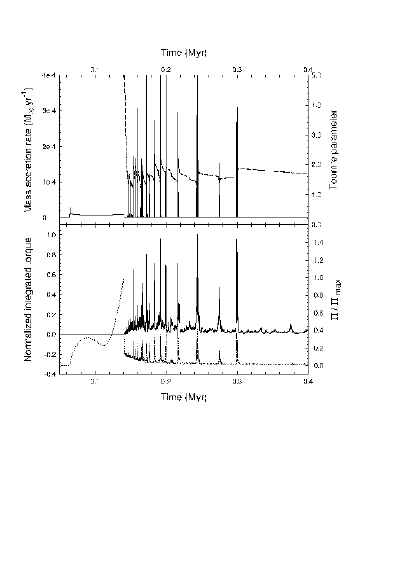
Figure 2: Evolution of model 2. Top: Temporal evolution of the mass accretion rate (solid line) and the $Q$-parameter (dashed line). Bottom: the normalized integrated torque $\cal{T}/{\cal{T}_{\rm max}}$ (solid line) and the normalized integrated radial acceleration $\Pi/\Pi_{\rm max}$ (dotted line).

Figure 2 (top) shows the temporal evolution of the mass accretion rate (solid line) and the Toomre $Q$-parameter (dashed line), whereas Figure 2 (bottom) shows the normalized integrated gravitational torque $\cal{T}$ (solid line) and the normalized integrated radial acceleration $\Pi$ (dotted line). For our purpose, we are interested in a global property of the disk (instead of concentrating on local variations), so we calculate an approximate global value of $Q=\tilde{c}_{\rm s}\Omega/\pi G\Sigma$ by averaging $\tilde{c}_{\rm s}$, $\Omega$, and $\Sigma$ over all computational cells. The quantity $\tilde{c}_{\rm s}\equiv\sqrt{d{\cal P}/d\Sigma}$ is the effective sound speed. We calculate $\cal{T}$ as the sum of the absolute values of the individual torques $\tau=-m_{\rm c}(r,\phi)\,\partial\Phi/\partial\phi$ over all computational cells, and $\Pi$ as the sum of the absolute values of individual local accelerations $|\partial v_{r}/\partial r|$ over all cells. Here, $m_{\rm c}(r,\phi)$ is the gas mass in a cell with the polar coordinates $(r,\phi)$. Figure 2 (top) demonstrates that the temporal behavior of $\dot{M}$ after protostar formation at $t\approx 0.06$ Myr has two distinct modes, as shown in Paper I. In the earlier smooth mode, the behavior of $\dot{M}$ is very similar to that of the nonrotating model 1. The mass accretion rate stays near $10^{-5}~{}M_{\odot}$ yr^-1, except for a short period after the protostar formation at $t\approx 0.06$ Myr when $\dot{M}$ is nearly a factor of 3 greater. The later burst mode starts at $t\approx 0.14$ Myr, when a centrifugal disk forms and the accretion rate abruptly drops down to a very small value $\dot{M}\lesssim 10^{-7}~{}M_{\odot}$ yr^-1. The subsequent evolution is characterized by very short ($<100$ yr) but vigorous [$\dot{M}=(1-10)\times 10^{-4}~{}M_{\odot}$ yr^-1] accretion bursts, which are intervened by longer periods ($\gtrsim 10^{3}$ yr) of quiescent accretion. The frequency of the bursts decreases noticeably with time and no bursts are seen after $t\approx 0.3$ Myr.

As we demonstrated in Paper I, the accretion bursts occur when the dense clumps (henceforth, we often identify them as protostellar/protoplanetary embryos, or simply as embryos) are driven onto the protostar by the gravitational torques of spiral arms which develop in the disk. The temporal evolution of the Toomre parameter $Q$, the integrated torque $\cal{T}$, and the integrated radial acceleration $\Pi$ proves this scenario. The $Q$-parameter may serve as an approximate stability criterion since gas disks are gravitationally unstable to local nonaxisymmetric perturbations if $Q\leq 1.5-1.7$ (Polyachenko et al., 1997; Nelson et al., 1998; Boss, 1998), while $\cal{T}$ may roughly express the efficiency of angular momentum and mass redistribution by spiral inhomogeneities in the disk (Tomley et al., 1994). The dashed line in Figure 2 (top) shows that the Toomre parameter drops below a critical value just before the burst, indicating the onset of gravitational instability. The integrated torque shown in Figure 2 (bottom) grows before the burst and reaches a maximum value at the time of the burst, suggesting an increase in the efficiency of the radial redistribution of angular momentum (and mass). An increase in the radial redistribution of mass just before the burst is also implied by the correlation between the position of bursts in Figure 2 (bottom) and the maxima in the integrated radial acceleration, since the latter may roughly express the degree of centrifugal disbalance in the disk.

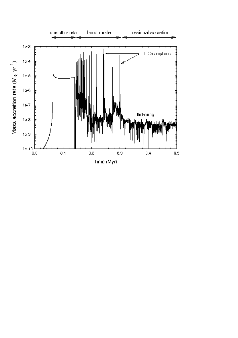
Figure 3: Temporal evolution of the mass accretion rate in model 2. A log scale is used to emphasize the low-amplitude flickering between the bursts and in the late evolutionary stage.

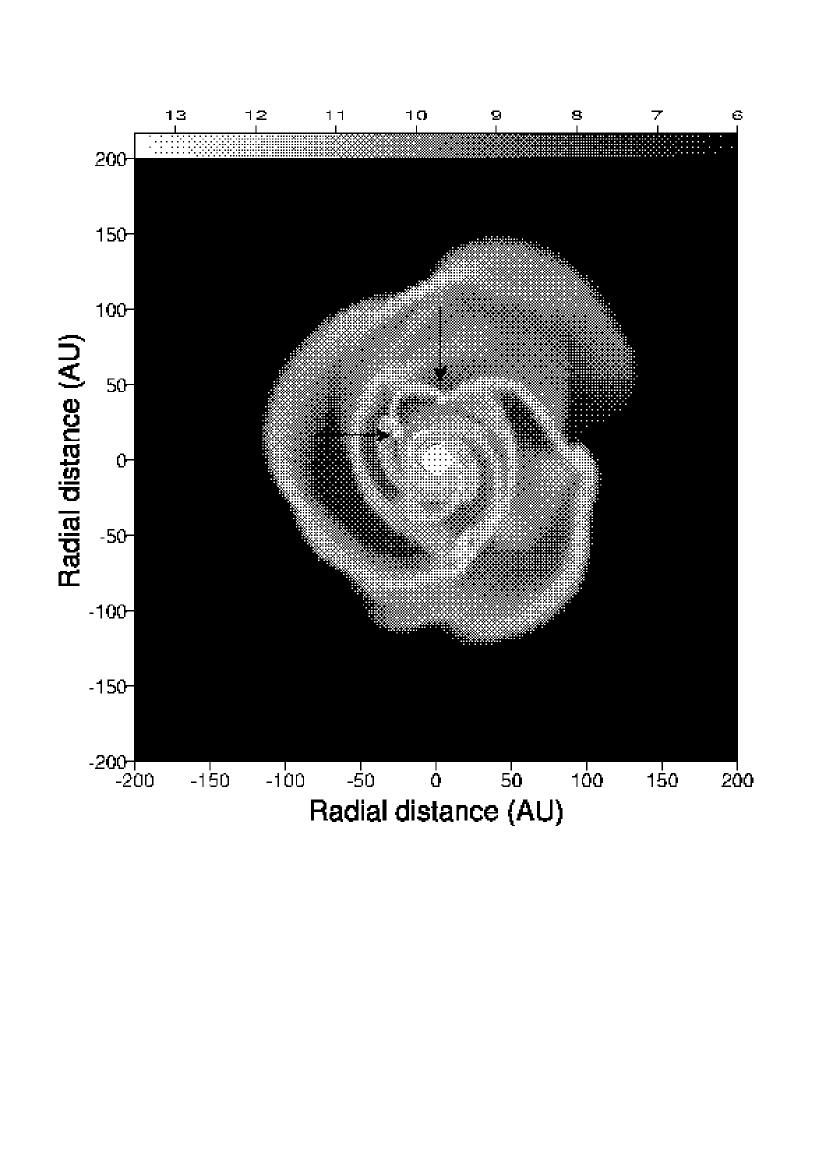
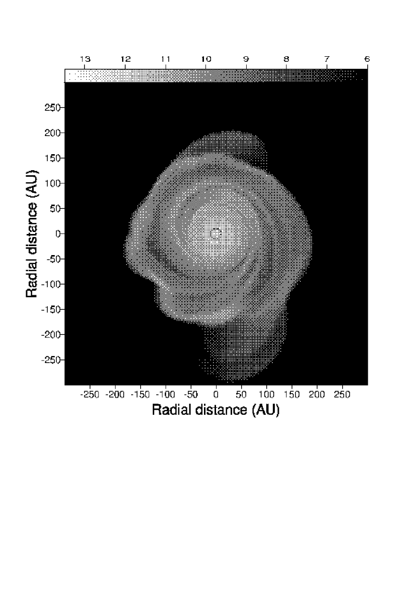
Figure 4: Image of the protostellar disk showing the gas volume density distribution in model 2 immediately preceding a mass accretion burst (left) and in the quiescent phase between the bursts (right). The protostellar/protoplanetary embryos with $n\gtrsim 10^{13}$ cm^-3 are indicated in the left image with the arrows. The scale bar is in cm^-3. A bright circle in each image represents the protostar plus some circumstellar matter.

We use a log scale to plot in Figure 3 the mass accretion rate obtained in model 2. The log scale emphasizes the low-amplitude flickering in the burst mode and during the late phase of residual accretion. Note that the flickering occurs after the protostellar disk forms around the protostar and it is absent during the smooth mode of accretion. The low-amplitude variations in $\dot{M}$ can be caused by gravitational torques of flocculent spiral arms (see Figure 4 for an example of spiral structure in the disk). We note that Figure  3 bears a remarkable resemblance to the empirically inferred schematic accretion history of young stars presented by Hartmann (1998, fig. 1.7).

To better illustrate the spiral structure and clump formation, we run model 2 at a higher resolution of $256\times 256$ grid points and plot the distribution of the gas surface density at two different times. Figure 4 (left) shows the spiral structure that immediately precedes a mass accretion burst. The formation of dense embryos with $n\gtrsim 10^{13}$ cm^-3 (shown by the arrows) within spiral arms is evident. The spiral structure is quite sharp and very chaotic, which is a consequence of the elevated mass and angular momentum redistribution and the onset of fragmentation. In contrast, during the quiescent phase of accretion the protostellar disk typically has a more uniform spiral pattern, as shown in Figure 4 (right). The spiral arms are smoother and more diffuse than in the period immediately preceding a burst.

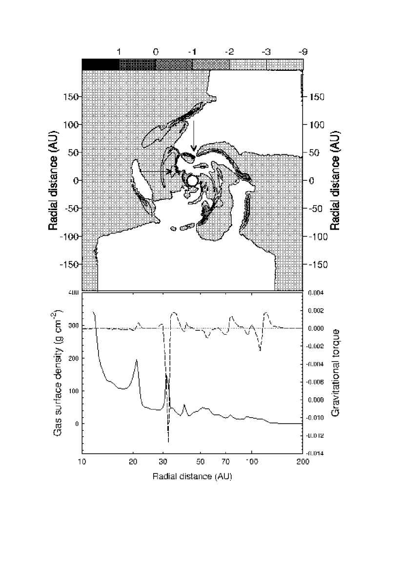
Figure 5: (Top) Spatial distribution of the negative gravitational torque $\tau$ (by absolute value) corresponding to the gas volume density distribution of Fig. 4 (left). The white space is characterized by positive $\tau$ (not shown in this image). The arrows point to the regions of maximum $\tau$ which coincide with the two clumps shown in Fig. 4 (left). The central circle represents the protostar plus some circumstellar matter. The scale bar is in dimensionless units and the conversion factor is $8.66\times 10^{40}~{}{\rm dyne}\cdot{\rm cm}$. (Bottom) Azimuthally averaged radial profiles of the surface density (solid line) and gravitational torque (dashed line) obtained from the spatial distribution of these quantities shown in Fig. 4 (left) and the top panel of this figure, respectively.

While the integrated (by absolute value) gravitational torque $\cal{T}$ expresses the efficiency of angular momentum and mass redistribution in the disk as a whole, the individual (local) gravitational torques $\tau=-m_{\rm c}(r,\phi)\,\partial\Phi/\partial\phi$ can provide physical insight into the temporal behavior of local density inhomogeneities. In general, the inhomogeneities that are characterized by negative $\tau$ are losing angular momentum and spiraling onto the protostar, while the inhomogeneities that are characterized by positive $\tau$ are gaining angular momentum and are moving radially outward. Figure 5 (top) shows the spatial distribution of $\tau$ computed at the same evolutionary time as the gas surface density distribution in Figure 4 (left). Only regions of negative $\tau$ have the absolue values plotted on a log scale, while the regions of positive $\tau$ are left as white space. It is evident that the density enhancements are usually (but not always) distinguished by the negative gravitational torques. The largest negative torques are found at the positions of the two clumps shown in Figure 5 (top) and Figure 4 (left) by the arrows. Note that a large portion in the upper-right part of Figure 5 (top) is characterized by positive torques, implying a local exchange of angular momentum between the clumps and this part of the disk. In some cases, the radial profiles of the azimuthally averaged gravitational torque $\tau(r)$ and the azimuthally averaged gas surface density $\Sigma(r)$ can better capture the physics behind the burst phenomenon; they are shown in Figure 5 (bottom). It is clearly seen that the largest negative torque is exerted on the gas density enhancement at $r\approx 32$ AU, which in fact corresponds to a dense clump shown in Figure 4 (left) by the horizontal arrow. This clump is caught in the process of a dramatic loss of its angular momentum and is currently spiraling down onto the protostar. In return, the gas at slightly larger radii $r\approx(32-40)$ AU is experiencing the positive gravitational torque and is currently moving outward. This is a nice example of the local angular momentum and mass redistribution mechanism that ultimately leads to the burst phenomenon. We note that the correlation of angular momentum transport with regions of high surface density fluctuation is qualitatively similar to the process described by Larson (1984).

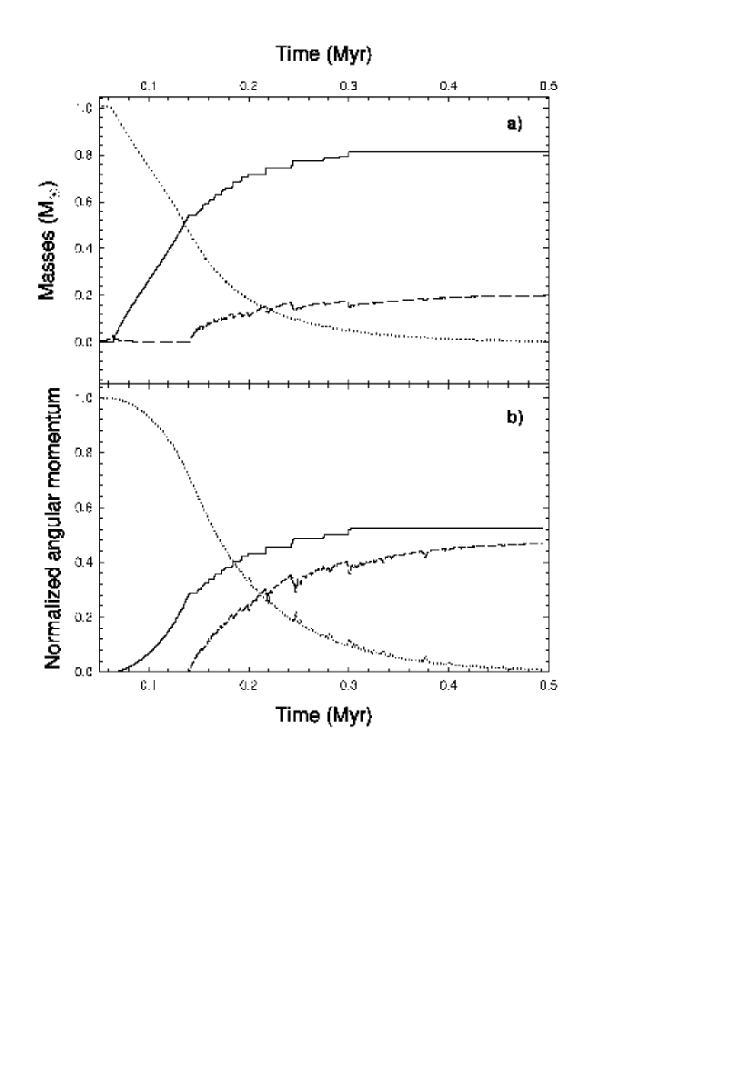
Figure 6: Temporal evolution of (a) the protostar mass (solid line), the envelope mass (dotted line), and the protostellar disk mass (dashed line) and (b) the protostellar angular momentum (solid line), envelope angular momentum (dotted line), and protostellar disk angular momentum (dashed line) in model 2. Note that the mass of the protostellar disk always stays well below that of the protostar. By the notion “protostar” we refer to the central 10 AU, which comprises the actual central object plus some circumstellar disk material.

Figure 6a shows the masses contained in the envelope (dotted line), the protostellar disk (dashed line), and the inner 10 AU (solid line) in model 2. We note that the inner 10 AU comprises the protostar and some circumstellar matter. The dynamics of this region is not resolved in our numerical simulations. However, the mass and total angular momentum contained within that region are accurately calculated using the mass and angular momentum fluxes through the inner boundary at 10 AU. Henceforth, we refer to the inner 10 AU as simply a protostar. The evolution is followed until approximately $99\%$ of the envelope has been absorbed by the protostar and the protostellar disk. We define the protostellar disk mass as that contained within the inner 200 AU; the material external to this distance is attributed to the envelope. This gives us upper and lower estimates for the disk and envelope masses, respectively. It is evident that every sharp increase in the protostellar mass (associated with the infall of embryos) correlates with a corresponding decrease in the mass of the disk, which remains well below the mass of the protostar during the evolution. Approximately $0.01~{}M_{\odot}-0.05~{}M_{\odot}$ is absorbed during each mass accretion burst. The accretion bursts cease at $t=0.3$ Myr, when the initial envelope mass has dropped by roughly $95\%$ and the mass accretion rate onto the protostellar disk (measured at $r=600$ AU) has decreased to $6\times 10^{-7}~{}M_{\odot}$ yr^-1. In contrast, the accretion rate is $7.5\times 10^{-6}~{}M_{\odot}$ yr^-1 at the beginning ($t=0.15$ Myr) of the burst mode of accretion. Figure 6b shows the normalized total angular momenta of the envelope (dotted line), the protostellar disk (dashed line), and the protostar (solid line), respectively, in model 2. We calculate the total angular momentum of the disk as the sum of the individual angular momenta $m_{\rm c}\Omega\,r^{2}$ in the inner 200 AU; the individual angular momenta external to this distance are attributed to the total angular momentum of the envelope. The comparison of the top and bottom panels in Figure 6 reveals a striking difference in the temporal evolution of masses and total angular momenta of the protostar and protostellar disk. At $t=0.5$ Myr, when the envelope has lost more than $99\%$ of its mass and angular momentum, the protostar has gained almost 80% of the total mass but only $55\%$ of the total angular momentum. In contrast, the protostellar disk has gained at the same time only $20\%$ of the total mass but almost $45\%$ of the total angular momentum. This is a powerful confirmation of the angular momentum redistribution in the protostellar disk, which we attribute to the gravitational torques of spiral arms. The fact that the protostar has gained approximately $55\%$ of the total angular momentum after 0.5 Myr may seem excessive. However, we note that we do not resolve the protostar itself. This amount of angular momentum is in fact contained in the inner 10 AU, which includes not only the protostar but some circumstellar matter as well. The distribution of angular momentum within the inner 10 AU remains beyond the scope of our present calculations. We further note that the thin-disk approximation does not take into account the powerful mechanism of angular momentum loss by protostellar winds, which would ultimately take away a considerable portion of the angular momentum in the inner 10 AU. Finally, we want to stress that the sum of all masses and angular momenta in Figure 6 remain practically constant during the evolution, indicating an excellent global conservation of mass and angular momentum in our numerical simulation.

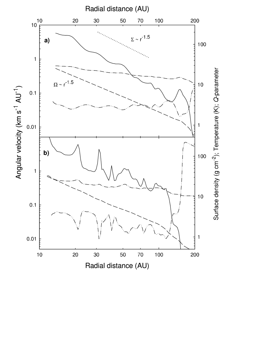
Figure 7: Radial profiles of surface density (solid lines), angular velocity (dashed lines), temperature (dash-dotted lines), and $Q$-parameter (dash-double-dotted lines) corresponding to (a) the gas distribution in the quiescent phase shown in Fig. 4 (right) and (b) to the gas distribution in the burst phase shown in Fig. 4 (left). Note that the rotation is nearly Keplerian in both cases.

In order to get a better understanding of the physical conditions in the disk, we plot in Figure 7a and Figure 7b the azimuthally averaged radial profiles of surface density $\Sigma$ (solid lines), angular velocity $\Omega$ (dashed lines), temperature $T$ (dash-dotted lines), and $Q$-parameter (dash-double-dotted lines) in the quiescent and burst phases, respectively. More specifically, the radial profiles in Figure 7a correspond to the gas distribution shown in Figure 4 (right), while the radial profiles in Figure 7b are obtained from the gas distribution of Figure 4 (left). The radial profiles of $\Omega$ and $T$ are similar during the burst and quiescent phases. The disk rotation is nearly Keplerian, $\Omega\propto r^{-1.5}$, as can be expected from the ratio of disk to protostar masses in Figure 6. The radial temperature profile shows a mild increase towards the center from 10 K at 200 AU to approximately 30 K at 15 AU. The biggest differences are seen in the radial surface density distribution – the quiescent phase is characterized by a much smoother profile with $\Sigma\propto r^{-1.5}$. The radial surface density profile in the burst phase has multiple peaks, some of which correspond to the forming protoplanetary embryos. The profiles in both the burst and quiescent phases have sharply defined boundaries at approximately 200 AU where the disk merges with the infalling envelope. Since the radial profiles of $\Omega$ and $T$ are quite similar in the burst and quiescent phases, the radial distribution of the $Q$-parameter is mostly determined by the radial variations in $\Sigma$. As a consequence, the $Q$-profile is much smoother and its values are noticeably larger in the quiescent phase than in the burst phase. During the burst phase, both the peaks in $\Sigma$ within the inner disk ($<40$ AU) and most of the outer disk are characterized by $Q\approx 1.0-1.5$. During the quiescent phase, $Q$ falls in the range $2.5-3.0$ and never goes below 2.0. The existence of gravitational instability is usually not expected at such high values of $Q$. Nevertheless, a weak spiral structure can be clearly seen in Figure 4 (right), which shows the gas volume density distribution during the quiescent phase. This indicates that once the spiral structure is generated during the burst phase, there exists an amplification mechanism (or mechanisms) that sustains at least a low level of this structure for a substantially long time. Strong observational evidence for the existence of spiral structure in the several-million-year-old disks around AB Aurigae (Fukagawa et al., 2004) and HD 100546 (Grady et al., 2001) tend to support this conjecture.

3.2.1 The effect of different rotational energy

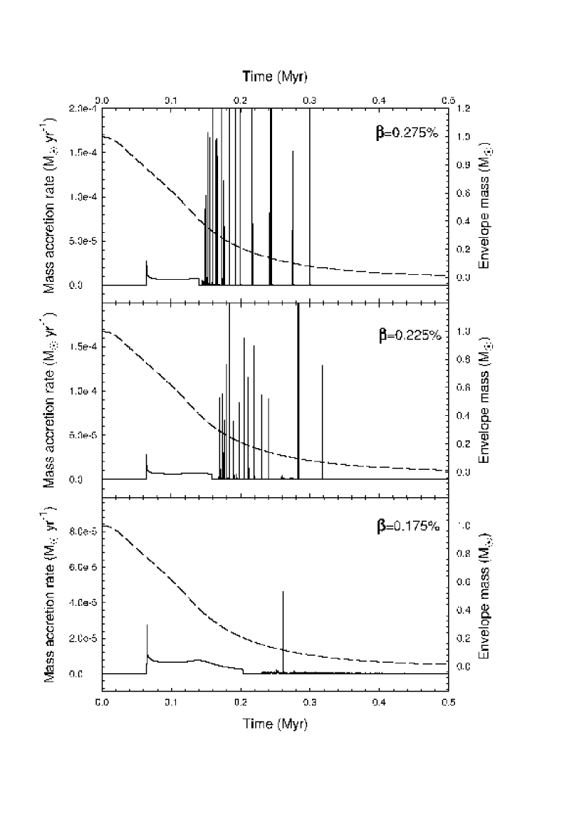
Figure 8: Temporal evolution of the mass accretion rate (solid lines) and envelope mass (dashed lines) for models with different values of $\beta$. Model 2 (top panel), model 3 (middle panel), and model 4 (bottom panel) have values of $\beta$ as indicated in each panel.

As we have shown, rotation introduces a qualitatively distinct mode into the evolution of mass accretion onto the protostar: a burst mode. In this subsection, we investigate the effect that the different initial rotational energies of cloud cores may have on the frequency, number, and amplitude of mass accretion bursts. For comparison with model 2, we present model 3 and model 4, which have different initial rotation energies than model 2 but are otherwise identical. The parameters of these models are listed in Table 1. Since all three models have the same initial gravitational energy, it is useful to differentiate the models by $\beta$, the ratio of magnitudes of initial rotational and gravitational energy. The solid lines in the top, middle, and bottom panels of Figure 8 show the temporal evolution of the mass accretion rate obtained in model 2, model 3, and model 4, respectively. In each figure, the dashed lines show the instantaneous envelope mass. A decrease in $\beta$ has a profound effect on the bursts. The $\beta=0.225\%$ model 3 has noticeably fewer and less vigorous bursts. A further decrease to $\beta=0.175\%$ (model 4) almost eliminates the bursts.

This tendency can be understood if we consider the three phases of mass accretion onto the protostar in the case of nonrotating cloud cores. We have emphasized in § 3.2 that the temporal behavior of $\dot{M}$ is very similar in rotating and nonrotating models before the formation of the protostellar disk. In the $\beta=0.275\%$ model 2, the disk forms in the intermediate accretion phase when the infall rate onto the disk is near-constant and equals $\approx 7.5\times 10^{-6}~{}M_{\odot}$ yr^-1. The envelope at the time of the protostellar disk formation is massive enough ($\approx 45\%$ of the total mass) to continuously supply the disk with matter for $0.1-0.2$ Myr. With an infall rate of $\lesssim 7.5\times 10^{-6}~{}M_{\odot}$ yr^-1 onto the disk, it takes $\gtrsim 10^{3}$ yr for the disk to accumulate $\approx 0.01~{}M_{\odot}$. The frequency of the mass accretion bursts decreases as the infall rate onto the disk diminishes during the evolution. In the $\beta=0.225\%$ model 3, the disk forms just after the terminal accretion phase has begun, and the frequency of bursts is somewhat less than in model 2. The accretion rate $\dot{M}$ exceeds $2\times 10^{-4}~{}M_{\odot}$ yr^-1 in only two episodes as compared to eight episodes in the $\beta=0.275\%$ model 2. Furthermore, in the $\beta=0.175\%$ model 4, the protostellar disk forms late in the terminal accretion phase, i.e., when most of the total envelope mass has already been accreted by the protostar and protostellar disk. Consequently, the infall rate onto the disk is low ($\approx 2\times 10^{-6}~{}M_{\odot}$ yr^-1) and quickly decreases further. The protostellar disk stays near the borderline of stability and provides a relatively smooth accretion of matter onto the protostar, punctuated by only a single mass accretion burst.

The size of a cloud core also affects the frequency of bursts since it determines the duration of the intermediate (near-constant) accretion phase. The larger a cloud, the longer the duration of the intermediate phase since the inward propagating rarefaction wave from the outer boundary takes a longer time to affect the protostar. The centrifugal radius $r_{\rm cf}$ of a gas parcel located initially at a distance $r$ can be estimated by assuming that all mass inside $r$ is concentrated in a central point source of mass $M$. In this case $r_{\rm cf}=K^{2}/GM$ where $K$ is the specific angular momentum of the gas parcel. Consequently, two clouds with identical density and rotation profiles but different sizes will form the protostellar disk at nearly the same time but in different accretion phases. The larger cloud will have a longer intermediate phase of accretion onto the disk, which will drive more vigorous burst activity.

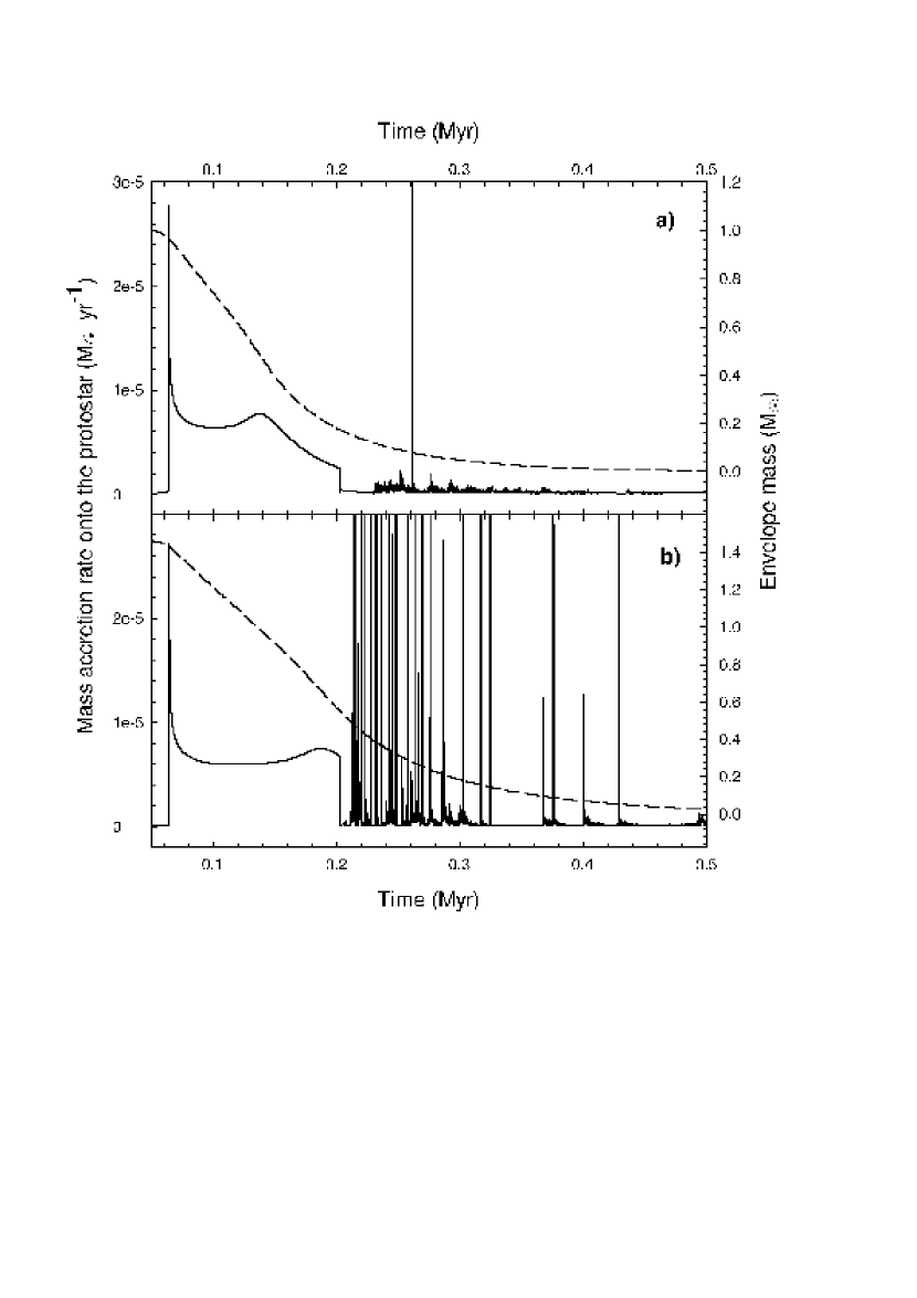
Figure 9: Temporal evolution of the mass accretion rate (solid lines) and envelope mass (dashed lines) for ($a$) model 4, and ($b$) model 5. The model 5 cloud core has the same initial central rotation rate as model 4 but has a greater mass.

Figures 9a and 9b show the temporal behavior of the mass accretion rate onto the protostar (the solid lines) and the corresponding envelope masses (the dashed lines) in model 4 and model 5, respectively. Both models have identical parameters except that the size of the cloud core in model 5 is larger than in model 4. More specifically, model 4 has $r_{\rm out}=10^{4}$ AU (and $M_{\rm c}=1~{}M_{\odot}$), whereas model 5 has $r_{\rm out}=1.4\times 10^{4}$ AU (and $M_{\rm c}=1.5~{}M_{\odot}$). In both models, the protostellar disk forms at approximately 0.2 Myr. However, model 5 has just entered the terminal accretion phase and still has a fairly massive envelope ($0.5~{}M_{\odot}$), while model 4 is in the late part of the terminal accretion phase and has little mass left in the envelope ($\lesssim 0.1M_{\odot}$). As a result, model 5 shows multiple mass accretion bursts due to a high mass infall rate ($\lesssim 7\times 10^{-6}~{}M_{\odot}$ yr^-1) onto the protostellar disk, whereas model 4 develops a burst only once.

3.3 Effect of a frozen-in magnetic field in rotating cloud cores

We include the effect of a magnetic field through the assumptions of flux-freezing and a spatially uniform mass-to-flux ratio $\Sigma/B_{z}$, i.e., the quantity $\alpha$ in equation (13) is constant. In this case, the magnetic tension acts as a simple dilution of gravity and the magnetic pressure is a multiple of the gas pressure, as discussed in § 2.1. This implies that the critical value of the Toomre $Q$-parameter in our magnetized disk models should be lower than in nonmagnetized disks.

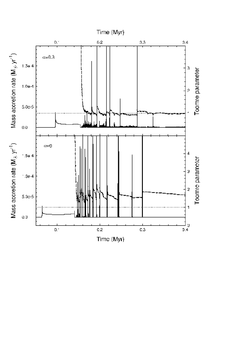
Figure 10: Temporal behavior of the mass accretion rate (solid lines) and the $Q$-parameter (dashed lines). Shown are model 6 (top), which has $\alpha=0.3$, and model 2 (bottom), which has $\alpha=0$. The dotted line denotes $Q=1$ and demonstrates that the magnetized model 6 needs to attain a lower value of $Q$ for instability to occur than does the unmagnetized model 2.

We simulate a magnetized cloud core with $\alpha=0.3$, hereafter called model  6, which is otherwise identical to the nonmagnetized model 2. The ratio of magnetic acceleration to gravity is $a_{\rm M}/|g_{r}|=\alpha^{2}(1+2\,a_{\rm T}/|g_{r}|)$, which equals 0.217 at small radii for $\alpha=0.3$. Figure 10 shows the temporal evolution of the mass accretion rate (solid lines) and the $Q$-parameter (dashed lines) in model 6 (the top panel), and in model 2 (the bottom panel). The dotted line draws the theoretical borderline of stability of nonmagnetized gas disks to axisymmetric perturbations ($Q=1$). It is evident that an increase in the magnetization of the cloud cores delays the formation of the protostar and moderates the burst activity.

Can the moderated burst activity in the magnetized model be understood in terms of the remaining envelope mass when the disk forms, as in the case of models with different levels of rotation? Comparing the two models, we find that they have comparable envelope masses at the time of disk formation. In fact, the magnetized model has a slightly more massive envelope ($0.52~{}M_{\odot}$) than does the nonmagnetized model ($0.45~{}M_{\odot}$). This is due to the fact that magnetized disks can support larger envelopes than their nonmagnetized counterparts. Therefore, the decreased burst activity in the magnetized disk cannot be attributed to a smaller envelope and mass accretion rate. Instead, it is an increased intrinsic stability of magnetized disks that is the key factor that moderates the mass accretion bursts.

The temporal behavior of the Toomre $Q$-parameter in Figure 10 proves our expectations that the magnetized disks are in general more stable than their nonmagnetized counterparts. In the magnetized model 6, the bursts occur at $Q\approx 0.9$, whereas in the nonmagnetized model 2, the bursts occur when $Q\approx 1.4$. The latter is in approximate agreement with previous results on the instability of nonmagnetized disks to nonaxisymmetric perturbations (e.g., Polyachenko et al., 1997; Nelson et al., 1998; Boss, 1998). The magnetized disks need to attain a lower value of $Q$ in order to be destabilized, fragment into dense clumps, and produce mass accretion bursts.

3.4 The isothermal-adiabatic transition and ratio of specific heats

The thermal evolution of a protostellar disk is determined by equation (8). The transition between the isothermal and adiabatic regimes is controlled by the critical density $\Sigma_{\rm cr}$, which can be determined by comparison with radiation transfer simulations of gravitational collapse.

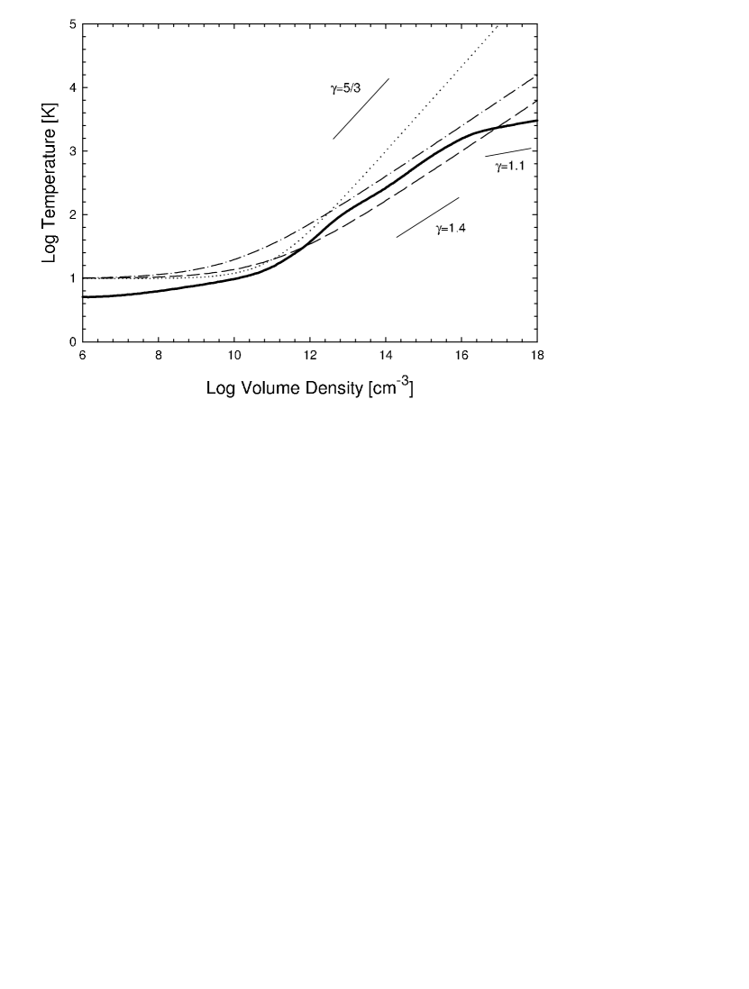
Figure 11: Comparison of the density-temperature relation (8) for $\Sigma_{\rm cr}=36.2$ g cm^-2 and $\gamma=1.4$ (dashed line), $\Sigma_{\rm cr}=11.6$ g cm^-2 and $\gamma=1.4$ (dash-dotted line), and $\Sigma_{\rm cr}=36.2$ g cm^-2 and $\gamma=5/3$ (dotted line) with the calculated density-temperature relation (thick solid line) of Masunaga & Inutsuka (2000) from radiation transfer simulations of the gravitational collapse of a molecular cloud core.

Figure 11 compares our density-temperature relation with that calculated by Masunaga & Inutsuka (2000, hereafter MI) using spherically symmetric frequency-dependent radiation transfer simulations. The dashed line shows equation (8) for $\Sigma_{\rm cr}=36.2$ g cm^-2 ($n_{\rm cr}=10^{11}$ cm^-3), whereas the dash-dotted line shows it for $\Sigma_{\rm cr}=11.6$ g cm^-2 ($n_{\rm cr}=10^{10}$ cm^-3). The thick solid line gives the density-temperature dependence as derived by MI. It is evident that $n_{\rm cr}=10^{10}$ cm^-3 and $n_{\rm cr}=10^{11}$ cm^-3 may be considered to be limiting values for the critical density, since most of MI’s density-temperature curve lies between the curves specified by these critical values. An obvious failure of the polytropic curves to embrace MI’s curve at $n<10^{11}$ cm^-3 is caused by a lower initial temperature (5 K) in MI’s simulations than our assumption of 10 K. We note that MI’s density-temperature dependence is derived for spherical collapse and it may differ in case of flattened cloud cores.

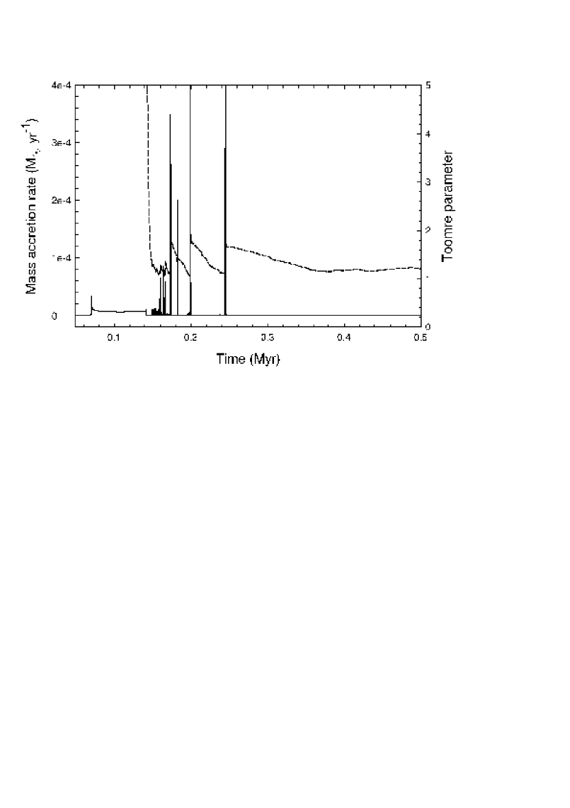
Figure 12: Temporal evolution of the mass accretion rate (solid line) and $Q$-parameter (dashed line) in model 7, which has the same parameters as model 2 but a lower value of $\Sigma_{\rm cr}$ ($=11.6$ g cm^-2).

In the models already presented, we have used $\Sigma_{\rm cr}=36.2$ g cm^-2. For a smaller value of $\Sigma_{\rm cr}$, the disk should be (on average) hotter and less susceptible to the development of gravitational instability and formation of protostellar/protoplanetary embryos. Consequently, the frequency and number of the mass accretion bursts is expected to decrease. Indeed, the solid line in Figure 12 shows the evolution of $\dot{M}$ in model 7, which has $\Sigma_{\rm cr}=11.6$ g cm^-2 ($n_{\rm cr}=10^{10}$ cm^-3). The parameters of model 7 are otherwise identical to the previously studied model 2 (see Table 1). A comparison of Figures 2 and 12 reveals that the number of bursts has decreased by roughly a factor of 3. We conclude that a decrease in $\Sigma_{\rm cr}$ and an associated increase in the overall disk temperature, within realistic bounds, can moderate the protostellar/protoplanetary embryo formation (and related burst activity) but not completely suppress it.

The ratio of specific heats $\gamma$ that enters the polytropic law (7) will regulate the thermal evolution of the protostellar disk in the optically thick regime. The cloud cores consist mostly of molecular hydrogen, which is a diatomic gas with $\gamma=7/5=1.4$. The dashed and dash-dotted lines in Figure 11 demonstrate that $\gamma=1.4$ reproduces, for the most part, the slope of the density-temperature relation from the simulations of MI. However, if the gas temperature is low, neither rotational nor vibrational modes of molecular hydrogen are excited and $\gamma$ becomes equal to 5/3.

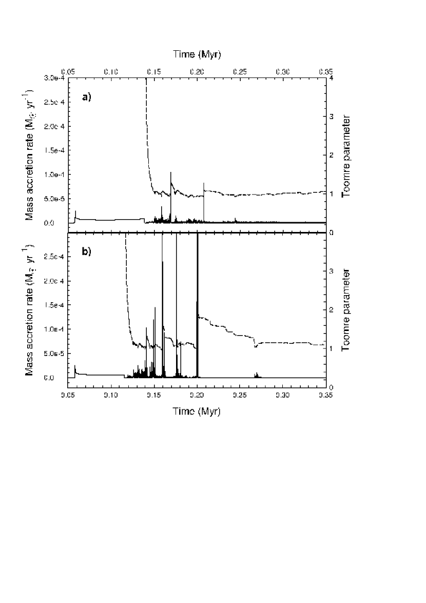
Figure 13: Temporal evolution of the mass accretion rate (solid line) and $Q$-parameter (dashed line). ($a$) Model 8, which has the same parameters as model 2 but a higher value of $\gamma=5/3$. ($b$) Model 9, which is identical to model 8 but has a higher initial rotational energy, i.e., $\beta=0.4\%$

The polytropic density-temperature relation (8) with $\gamma=5/3$ and $\Sigma_{\rm cr}=36.2$ g cm^-2 ($n_{\rm cr}=10^{11}$ cm^-3) is shown in Figure 11 by the dotted line. It is a reasonable fit to the results of MI (thick solid line) in the density range $n=10^{11}{\rm cm}^{-3}-10^{13}{\rm cm}^{-3}$ but yields much greater temperatures at higher densities. This can result in an additional heating of the protostellar disk in the optically thick regime and may suppress the formation of dense protostellar/protoplanetary embryos. The solid line in Figure 13a shows the evolution of the mass accretion rate in model 8, which has the same parameters as model 2 but $\gamma=5/3$. It is evident that an increased $\gamma$ considerably reduces the burst activity – only two moderate-amplitude bursts with $\dot{M}\lesssim 10^{-4}~{}M_{\odot}$ yr^-1 are now seen, in comparison to sixteen in model 2.

The suppressive effect of an elevated $\gamma$ (and by implication greater disk temperature) on the embryo formation can be compensated to some extent by a greater infall rate onto the protostellar disk. We demonstrate this by introducing a new model 9, which has a higher initial rotational energy ($\beta=0.4\%$) but is otherwise identical to model 8 ($\beta=0.275\%$). Given an increased initial rotational energy, the protostellar disk forms at an earlier time and when the envelope mass is greater. The solid line in Figure 13b shows the mass accretion rate onto the protostar $\dot{M}$ obtained in the $\beta=0.4\%$ model 9. It is clear that the burst activity is greatly enhanced over that of the $\beta=0.275\%$ model 8. The difference in the envelope mass at the time of the disk formation in the two models is substantial: the $\beta=0.4\%$ model 9 has approximately $63\%$ of its total mass in the envelope while the $\beta=0.275\%$ model 8 has only $46\%$. Consequently, model 9 can sustain a high infall rate onto the protostellar disk for a longer time than model 8, which favors the formation of dense clumps and associated burst activity.

4 Discussion

Our parameter survey reveals that the basic mechanism of burst formation is robust and occurs under a variety of circumstances. Gravitational instability in the disk is driven by continuing infall from the envelope, which leads to spiral arms which fragment to form dense clumps. Our long-term integration reveals that the fate of these clumps is to be driven onto the protostar, due to gravitational torques from their interaction with the disk, especially the spiral arms.

It is possible that disk heating sources (external, protostellar, or internal, e.g., shocks or compression) coupled with less efficient cooling may suppress the formation of the clumps. However, we find that the basic mechanism occurs even in models with either a low value of $\Sigma_{\rm cr}$ or with $\gamma=5/3$, both of which overestimate the gas temperature relative to that obtained in spherically symmetric radiative transfer calculations (see Fig. 11). The strength and frequency of the bursts is certainly dependent on the disk thermodynamics, but also depends crucially on the envelope mass at the time of disk formation, since this process is ultimately driven by the mass accretion from the envelope. We believe, on theoretical grounds, that the burst mode will occur as a part of the collapse of most (if not all) cloud cores, consistent with the observational source statistics of FU Ori objects, which imply that every young star undergoes some 10-20 bursts during its lifetime (Hartmann & Kenyon, 1996).

Why has the burst mode of accretion not been discovered in any numerical simulations of disk evolution prior to our Paper I? We believe that there are two reasons: (1) our model calculates the formation of a disk self-consistently from the collapse of a cloud core, and its continuing evolution as influenced by infall from the remnant core envelope; (2) we are able to carry out a long-term time integration (at least a few $\times 10^{5}$ yr after disk formation), in order to settle the fate of the clumps after they are formed. Both of these advances are facilitated by our use of the two-dimensional thin-disk approximation, rather than three-dimensional simulations which are currently far more resource-limited.

Several other groups have recently developed global three-dimensional numerical models to study the onset of gravitational instability in isolated and marginally unstable disks. These simulations aim to understand whether gas giant planets can be formed by direct gravitational instability. Using either finite-difference (Boss, 2003; Pickett et al., 2003; Mejía et al., 2005) or smoothed-particle hydrodynamics (Rice et al., 2003; Mayer et al., 2004) techniques, and either isothermal evolution or various recipes for heating, radiative cooling, and simplified radiative transfer, these simulations often find that spiral structure gives birth to dense clumps as in our model. Clump formation is reduced in models with prescribed heating and cooling, and is even suppressed in some models (Mejía et al., 2005; Cai et al., 2006). All of the above models truncate the disk at an outer radius in the range of 20 AU to 40 AU, with no account of outside influence. Our view is that clump formation will likely occur in any of these situations if the significant infall from the envelope during the early disk evolution is included. However, another important question is the survivability of the clumps, if they do form. The three-dimensional simulations described above cannot follow the evolution for more than $\sim 10^{3}$ yr, and therefore cannot settle this issue. Our time-integration follows the disk evolution for $\gtrsim 10^{5}$ yr, and each clump is followed for many orbit times, until its fate is settled. Our simulations show that clumps are driven onto the protostar (or are dispersed in a minority of cases), so that there are no clumps remaining in the disk by the time that 99% of the envelope matter has been accreted. Furthermore, the gravitational instability has essentially ceased to operate by this late time. This casts doubt on the possibility of gas giant planet formation by direct gravitational instability. However, three-dimensional simulations and models which allow the protostar to move off-center are also necessary to confirm these results. We believe that further progress in this field will come from three-dimensional simulations of nonisolated disks which have a high resolution, span a large range of length scales, and also integrate to very late times (at least $10^{5}$ yr after disk formation). Increasingly sophisticated treatment of cooling, heating, and radiative transfer, as some groups have begun to do, are also essential for further progress.

The burst mode may hold the key to explaining the “luminosity problem” of class I protostars in Taurus described by Kenyon & Hartmann (1995); that is, the luminosities are much lower than predicted by the mass accretion rate $0.975\,c_{\rm s}^{3}/G$ of the standard Shu (1977) model. In an earlier paper (Vorobyov & Basu, 2005a), we explained the position of class 0 and class I protostars in a diagram of envelope mass $M_{\rm env}$ versus bolometric luminosity $L_{\rm bol}$ using evolutionary tracks from our spherical collapse models. These models had the early, intermediate, and terminal accretion phases, but no burst mode. The evolutionary tracks were in qualitative agreement with the position of class I objects since they provided an explanation for an apparent evolutionary decrease in $L_{\rm bol}$, due to the terminal accretion phase. (In contrast, steady accretion at a rate $\propto c_{\rm s}^{3}/G$ implies an indefinite increase in $L_{\rm bol}$.) However, we also noted in Vorobyov & Basu (2005a) that the model luminosities for Taurus class I sources were still significantly greater than observed (the problem was less severe for Ophiuchus class I sources). We believe that the further decrease in $L_{\rm bol}$ implied by the entry of the accretion into the quiescent phase of the burst mode may explain the remaining luminosity problem. Both the effect of a core boundary (which causes the terminal phase of accretion) and rotation (which introduces the burst mode) are likely needed to explain the luminosity problem. In other words, protostellar accretion needs to be understood conceptually as an interplay of the three phases of accretion (early, intermediate, and terminal - all of which exist in the absence of rotation) with the two modes of accretion (smooth mode and burst mode - the latter is introduced due to rotation). A detailed analysis of evolutionary tracks is left for a separate study.

The presence of a magnetic field is not necessary for the burst mode to occur at all, as the results in § 3.2 demonstrate. The magnetic field in a supercritical core can moderate the burst activity but not suppress it. In all models of collapse, whether it is induced by gravity, turbulence, or ambipolar diffusion, the magnetic field is expected to be below the critical value in order for collapse to ensue. Our initial state is based on the analytic best-fits to numerical models of supercritical core collapse (Basu, 1997), and reflect the approximate flux-freezing and a spatially uniform mass-to-flux ratio in the early stages. Both assumptions are expected to break down in the near-environment of a protostar, where significant magnetic flux redistribution will take place, due to a combination of ambipolar diffusion (Ciolek & Königl, 1998; Tassis & Mouschovias, 2005), ohmic dissipation (Li & McKee, 1996), and Hall diffusion (Wardle, 1999). A weakened magnetic field is likely to enhance the strength of the bursts, as a comparison of our model 2 and model 6 demonstrates. However, the magnetic flux-loss from the inner region can introduce other, more complex, effects. The outward movement of magnetic flux into regions where it is better coupled to the neutrals can introduce a magnetic “wall” which retards accretion for a time (Li & McKee, 1996; Ciolek & Königl, 1998; Tassis & Mouschovias, 2005). This wall leads to a time-varying (fluctuating by a factor $\sim 10$ above and below the mean value) accretion rate onto the protostar in the calculations of Tassis & Mouschovias (2005), who do not account for rotation or nonaxisymmetric effects. Future calculations will settle the extent to which nonaxisymmetric motions and magnetic interchange instability (Stehle & Spruit, 2002) can moderate such magnetically-induced accretion rate fluctuations. Inclusion of dynamics in the third dimension (perpendicular to the disk plane) is also critical to understand the full effect of magnetic fields, since there is expected to be significant magnetic braking (Krasnopolsky & Königl, 2002), collapse-driven outflow (Tomisaka, 2002), and magnetorotational instability (Fromang et al., 2005), all of which can play a role in the angular momentum evolution of the disk. The interaction of the stellar magnetic field with the disk gas and magnetic field is also important for gas accretion (Königl, 1991; Shu et al., 1994). All in all, the interplay of disk formation and evolution (as calculated in this paper) with the various magnetic effects described above can be clarified through a series of future multidimensional non-ideal MHD simulations.

5 Summary

We have used the thin-disk approximation to calculate the runaway collapse and protostellar accretion phase for an ensemble of cloud models, accounting for rotation, frozen-in magnetic fields, and various relations for the density-temperature dependence. We have elucidated the nature of the burst mode of accretion, first presented by Vorobyov & Basu (2005c). We find the following major results:

1. The collapse of flattened nonrotating cloud cores yield protostars whose mass accretion rate $\dot{M}$ is characterized by three phases: an early phase of declining $\dot{M}$, an intermediate phase of near-constant $\dot{M}$ (this phase does not occur if the core is sufficiently compact), and a terminal phase of declining $\dot{M}$ due to a finite mass reservoir. These results agree qualitatively with earlier results for the collapse of a spherical cloud.

2. The collapse of a rotating cloud core and self-consistent formation of a protostellar disk leads to mass accretion in two distinct modes: a smooth mode, which is like the accretion in the nonrotating model, followed by a burst mode which occurs upon the formation of a protostellar disk. It is characterized by prolonged periods of low accretion rate from the disk (the quiescent phases) that are punctuated by intense bursts of accretion during which most of the protostellar mass is accumulated. The accretion bursts are associated with the formation of dense protostellar/protoplanetary embryos, which are later driven onto the protostar by the gravitational torques that develop in the disk. Gravitational instability in the disk that is driven by continuing infall from the cloud core envelope is responsible for the recurrent embryo formation.

3. The burst phenomenon is quite sensitive to the amount of angular momentum in the cloud, and the bursts are more frequent and intense for greater values of $\beta$, the ratio of the magnitudes of rotational and gravitational energy. For sufficiently low $\beta$, the disk may form during the late part of the terminal accretion phase of the smooth mode, and the infall onto the disk is not sufficient to create bursts.

4. The effect of a frozen-in magnetic field that is weaker than gravity (i.e., the core is magnetically supercritical) is to moderate the burst activity but not to suppress it. Magnetized disks have an intrinsically lower value of the critical $Q$ parameter for gravitational instability, but are eventually driven unstable by infall from the envelope.

5. The effect of enhanced temperatures at high density, in accordance with (or actually exceeding) the results of detailed radiative transfer calculations for spherical clouds, is to moderate the burst activity but not to suppress it.

6. Even in cases where the burst activity is nearly suppressed, we find that it can be made vigorous by moderate increases in the cloud size or rotation rate. We conclude that the burst mode is a robust phenomenon which is likely to occur during the evolution of most (if not all) protostars.

Appendix A Numerical Tests

A first test is of the van Leer advection scheme. We test it on a “relaxation” problem, in which a thin disk of constant surface density is given a velocity field proportional to $r$ ($v_{r}=\nu_{0}r$), and the surface density is allowed to decrease. For this problem, the analytic solution to the continuity equation is $\Sigma(t)=\Sigma_{0}e^{-2\nu_{0}t}$ and it yields $\Sigma=6.14\times 10^{-6}\Sigma_{0}$ at $\nu_{0}t=6$, i.e., when the surface density has decreased by nearly six orders of magnitude. Our numerical code yields $\Sigma=5.98\times 10^{-6}\Sigma_{0}$ at this time for a resolution of 256 logarithmically spaced radial grid points, so that the relative error is only 2.6%.

An important concern for numerical studies of gravitational collapse is the ability of a code to conserve specific angular momentum. A comprehensive test problem of specific angular momentum conservation that covers advection as well as pressure and gravity terms in the momentum equations was designed by Norman et al. (1980). For a fluid with no mechanism for redistributing angular momentum, the mass $M(K)$ in the cloud core with specific angular momentum ($\Omega r^{2}$) less than or equal to $K$ is a constant of the motion. A deviation from the initial spectrum $M(K)$ reveals a redistribution of angular momentum. For a uniformly rotating cloud ($\Omega={\rm constant}$) with the radial surface density distribution given by equation (19), we have

$$M(K)=2\pi\Sigma_{0}r_{0}^{2}\left(\sqrt{1+{K\over K_{0}}}-1\right),$$ (A1)

where $K_{0}=\Omega r_{0}^{2}$. We consider a uniformly rotating ($\Omega=1.0$ km s^-1 pc^-1) cloud core with otherwise the same parameters as model 2. The initial theoretical spectrum $M(K)$ is shown in Figure 14 by the dashed line. The solid line plots $M(K)$ computed at $t=0.07$ Myr, which is $\approx 5000$ yr after the formation of the central protostar. At this time, the protostellar disk has not yet formed and the flow of gas onto the protostar proceeds in an axisymmetric manner. It is clear that $M(K)$ merges with the initial spectrum. This indicates virtually no angular momentum redistribution due to either physical or numerical reasons. We note that a part of the cloud core with low angular momentum has been accreted into the sink cell. When the protostellar disk forms at $t=0.107$ Myr, the gravitational torques associated with spiral arms produce a considerable deviation in the spectrum $M(K)$. This deviation is apparent in Figure 14, where we plot with crosses the spectrum at $t=0.115$ Myr.

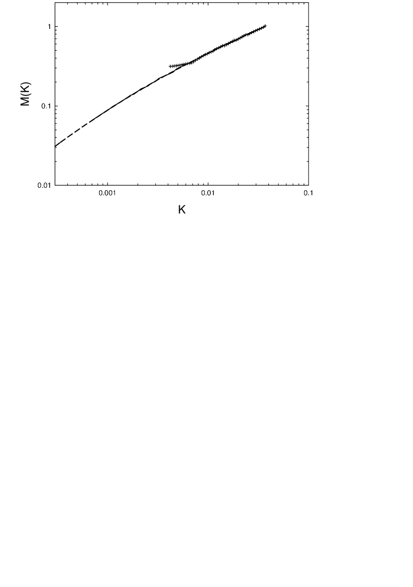
Figure 14: The specific angular momentum spectrum of a collapsing cloud core. The quantity $M(K)$ is the total mass in the cloud with specific angular momentum less than or equal to $K$. The dashed line shows the analytically derived spectrum of the initial state. The solid line shows $M(K)$ in our simulation after the formation of the protostar but before the formation of the protostellar disk. The crosses show the spectrum after the formation of the protostellar disk, and reveal the significant redistribution of angular momentum by nonaxisymmetric gravitational instabilities in the disk.

Table 1: Parameters of model cloud cores

Model	$r_{\rm out}$	$\Omega_{0}$	$\alpha$	$\gamma$	$\Sigma_{\rm cr}$
1	$10^{4}$	0	0	1.4	36.2
2	$10^{4}$	1.5	0	1.4	36.2
3	$10^{4}$	1.35	0	1.4	36.2
4	$10^{4}$	1.2	0	1.4	36.2
5	$1.4\times 10^{4}$	1.2	0	1.4	36.2
6	$10^{4}$	0	0.3	1.4	36.2
7	$10^{4}$	1.5	0	1.4	11.6
8	$10^{4}$	1.5	0	5/3	36.2
9	$10^{4}$	1.8	0	5/3	36.2

References

- Bacmann et al. (2000) Bacmann, A., André, P., Puget, J. L., et al. 2000, A&A, 314, 625
- Basu (1997) Basu, S. 1997, ApJ, 485, 240
- Basu & Mouschovias (1994) Basu, S., & Mouschovias, T. Ch. 1994, ApJ, 432, 720
- Basu & Mouschovias (1995a) . 1995a, ApJ, 452, 386
- Basu & Mouschovias (1995b) . 1995b, ApJ, 453, 271
- Bate et al. (2003) Bate, M. R., Bonnell, I. A., & Bromm, V. 2003, MNRAS, 339, 577
- Bell & Lin (1994) Bell, K. R., & Lin, D. N. C. 1994, ApJ, 427, 987
- Bell et al. (1995) Bell, K. R., Lin, D. N. C., Hartmann, L. W., & Kenyon, S. J. 1995, ApJ, 444, 376
- Binney & Tremaine (1987) Binney, J., & Tremaine, S. 1987, Galactic Dynamics (Princeton: Princeton Univ. Press)
- Bonnell & Bastien (1992) Bonnell, I., & Bastien, P. 1992, ApJ, 401, L31
- Boss (1998) Boss, A. P. 1998, ApJ, 503, 923
- Boss (2003) . 2003, ApJ, 599, 577
- Cai et al. (2006) Cai, K., Durisen, R. H., Michael, S., Boley, A. C., Mejía, A. C., Pickett, M. K., & D’Alessio, P. 2006, ApJ, 636, L149
- Ciolek & Königl (1998) Ciolek, G. E., & Königl, A. 1998, ApJ, 504, 257
- Ciolek & Mouschovias (1993) Ciolek, G. E., & Mouschovias, T. Ch. 1993, ApJ, 454, 194
- Clarke et al. (1990) Clarke, C. J., Lin, D. N. C., & Pringle, J. E. 1990, MNRAS, 242, 439
- Fatuzzo et al. (2004) Fatuzzo, M., Adams, F. C., & Myers, P. C. 2004, ApJ, 615, 813
- Fiedler & Mouschovias (1993) Fiedler, R. A., & Mouschovias, T. Ch. 1993, ApJ, 415, 680
- Foster & Chevalier (1993) Foster, P. N., & Chevalier, R. A. 1993, ApJ, 416, 303
- Fromang et al. (2005) Fromang, S., Balbus, S. A., Terquem, C., & De Villiers, J.-P. 2005, ApJ, 616, 364
- Fukagawa et al. (2004) Fukagawa, M., Hayashi, M., Tamura, M. et al. 2004, ApJ, 605, L53
- Grady et al. (2001) Grady, C. A., Polomski, E. F., Henning, Th., et al. 2001, AJ, 122, 3396
- Hartmann (1998) Hartmann, L. 1998, Accretion Processes in Star Formation (Cambridge: Cambridge Univ. Press)
- Hartmann & Kenyon (1996) Hartmann, L., & Kenyon, S. 1996, ARA&A, 34, 207
- Henriksen et al. (1997) Henriksen, R., André, P., & Bontemps, S. 1997, A&A, 323, 549
- Herbig (1977) Herbig, G. H. 1977, ApJ, 217, 693
- Hunter (1977) Hunter, C. 1977, ApJ, 218, 834
- Kenyon & Hartmann (1995) Kenyon, S. J., & Hartmann, L. 1995, ApJS, 101, 117
- Kenyon et al. (1990) Kenyon, S. J., Hartmann, L. W., Strom, K. M., & Strom, S. E. 1990, AJ, 99, 869
- Königl (1991) Königl, A. 1991, ApJ, 370, L39
- Krasnopolsky & Königl (2002) Krasnopolsky, R., & Königl, A. 2002, ApJ, 580, 987
- Larson (1984) Larson, R. B. 1984, MNRAS, 206, 197
- Larson (2003) . 2003, Rep. Prog. Phys. 66, 1651
- Laughlin & Bodenheimer (1994) Laughlin, G., & Bodenheimer, P. 1994, ApJ, 436, 335
- Li & McKee (1996) Li, Z.-Y., & McKee, C. F. 1996, ApJ, 464, 373
- Li & Shu (1997) Li, Z.-Y., & Shu, F. H. 1997, ApJ, 475, 237
- Lin & Papaloizou (1985) Lin, D. N. C., & Papaloizou, J. C. B. 1985, in Protostars and Planets II, ed. D. C. Black & M. C. Matthews (Tucson: Univ. Arizona Press), 981
- Masunaga & Inutsuka (2000) Masunaga, H., & Inutsuka, S. 2000, ApJ, 531, 350
- Masunaga et al. (1998) Masunaga, H., Miyama, S. M., & Inutsuka, S. 1998, ApJ, 495, 346
- Mayer et al. (2004) Mayer, L., Quinn, T., Wadsley, J., & Stadel, J. 2004, ApJ, 609, 1045
- Mejía et al. (2005) Mejía, A. C., Durisen, R. H., Pickett, M. K., & Cai, K. 2005, ApJ, 619, 1098
- Nakamura & Hanawa (1997) Nakamura, F., & Hanawa, T. 1997, ApJ, 480, 701
- Nakano & Nakamura (1978) Nakano, T., & Nakamura, T. 1978, PASJ, 30, 671
- Narita et al. (1984) Narita,, S. Hayashi, C., & Miyama, S. M. 1984, Prog. Theor. Phys., 72, 1118
- Nelson et al. (1998) Nelson, A. F., Benz, W., Adams, F. C., & Arnett, D. 1998, ApJ, 502, 342
- Norman et al. (1980) Norman, M. L., Wilson, J. R., & Barton, R. T. 1980, ApJ, 239, 968
- Pickett et al. (2003) Pickett, B. K., Mejía, A. C., Durisen, R. H., Cassen, P. M., Berry, D., & Link, R. P. 2003, ApJ, 590, 1060
- Polyachenko et al. (1997) Polyachenko, V. L., Polyachenko, E. V., & Strel’nikov, A. V. 1997, Astron. Zhurnal, 23, 551 (translated Astron. Lett. 23, 483)
- Rice et al. (2003) Rice, W. K. M., Armitage, P. J., Bate, M. R., & Bonnell, I. A. 2003, MNRAS, 339, 1025
- Shakura & Sunyaev (1973) Shakura, N. I., & Sunyaev, R. A. 1973, A&A, 24, 337
- Shu (1977) Shu, F. H. 1977, ApJ, 214, 488
- Shu & Li (1997) Shu, F. H., & Li, Z.-Y. 1997, ApJ, 475, 251
- Shu et al. (1994) Shu, F. H., Najita, J., Ostriker, E., Wilkin, F., Ruden, S., & Lizano, S. 1994, ApJ, 429, 781
- Stehle & Spruit (2002) Stehle, R., & Spruit, H. C. 2002, MNRAS, 323, 587
- Stone & Norman (1992) Stone, J. M., & Norman, M. L. 1992, ApJS, 80, 753
- Tassis & Mouschovias (2005) Tassis, K., & Mouschovias, T. Ch. 2005, ApJ, 618, 783
- Tomisaka (1996) Tomisaka, K. 1996, PASJ, 48, L97
- Tomisaka (2002) . 2002, ApJ, 575, 306
- Tomley et al. (1994) Tomley, L., Steiman-Cameron, T. Y., & Cassen, P. 1994, ApJ, 422, 850
- van Leer (1977) van Leer, B. 1977, JCP, 23, 276
- Vorobyov & Basu (2005a) Vorobyov, E. I., & Basu, S. 2005a, MNRAS, 360, 675
- Vorobyov & Basu (2005b) . 2005b, MNRAS, 363, 1361
- Vorobyov & Basu (2005c) . 2005c, ApJ, 633, L137 (Paper I)
- Wardle (1999) Wardle, M. 1999, MNRAS, 307, 849
- Ward-Thompson et al. (1999) Ward-Thompson, D., Motte, F., & André, P. 1999, MNRAS, 305, 143
- Whitworth & Ward-Thompson (2001) Whitworth, A. P., & Ward-Thompson, D. 2001, ApJ, 547, 317