The XMM-Newton survey of the ELAIS-S1 field. I: Number counts, angular correlation function and X-ray spectral properties.

Abstract

Aims. The formation and evolution of cosmic structures can be probed by studying the evolution of the luminosity function of AGNs, galaxies and clusters of galaxies and of the clustering of the X-ray active Universe, compared to the IR-UV active Universe.

Methods. To this purpose, we have surveyed with XMM-Newton the central $\sim 0.6$ deg² region of the ELAIS-S1 field down to flux limits of $\sim 5.5\times 10^{-16}$ ${\rm erg\leavevmode\nobreak\ cm}^{-2}\leavevmode\nobreak\ {\rm s}^{-1}$ (0.5-2 keV, soft band, S), $\sim 2\times 10^{-15}$ ${\rm erg\leavevmode\nobreak\ cm}^{-2}\leavevmode\nobreak\ {\rm s}^{-1}$ (2-10 keV, hard band, H), and $\sim 4\times 10^{-15}$ ${\rm erg\leavevmode\nobreak\ cm}^{-2}\leavevmode\nobreak\ {\rm s}^{-1}$ (5-10 keV,ultra hard band, HH).

Results. We detect a total of 478 sources, 395 and 205 of which detected in the S and H bands respectively. We identified 7 clearly extended sources and estimated their redshift through X-ray spectral fits with thermal models. In four cases the redshift is consistent with z=0.4. We have computed the angular correlation function of the sources in the S and H bands finding best fit correlation angles $\theta_{0}=5.2\pm 3.8$ arcsec and $\theta_{0}=12.8\pm 7.8$ arcsec, respectively. A rough estimate of the present-day correlation length r₀ can be obtained inverting the Limber equation and assuming an appropriate redshift distribution dN/dz. The results range between 12.8 and 9.8 h^-1 Mpc in the S band and between 17.9 and 13.4 h^-1 Mpc in the H band, with 30-40% statistical errors, assuming either smooth redshift distributions or redshift distributions with spikes accounting for the presence of significant structure at z=0.4. The relative density of the S band sources is higher near the clusters and groups at z$\sim 0.4$ and extends toward East and toward South/West. This suggests that the structure is complex, with a size comparable to the full XMM-Newton field. Conversely, the highest relative source densities of the H band sources are located in the central-west region of the field.

1 Introduction

One of the most challenging goals of modern cosmology is to understand how the structures in the Universe have been formed and evolved during the time. Both clusters of galaxies and Active Galactic Nuclei (AGNs) shine powerfully in the X-ray band and therefore X-ray surveys are the most efficient tool to both trace the evolution of the cosmic web from low to high redshift and investigate the correlation between the formation and light-up of supermassive black holes (SMBH) in AGNs and the formation and evolution of galaxies. X-ray surveys are less biased against obscured AGN than optical UV surveys and thus reach higher surface densities ($\sim 1000$ deg^-2 at the flux limits reachable by Chandra and XMM-Newton in 50-100 ksec) than even faint optical AGN surveys (e.g., the COMBO 17 survey reaches $\sim 200$ deg^-2 with magnitude limit R${{}_{<}\atop{}^{\sim}}24$, Wolf et al. 2004), and so they can be used to trace the Large Scale Structure (LSS) more efficiently than optical AGNs. While there is today no doubt that tight links and feedbacks do exist between SMBH activity and galaxy evolution and between galaxy activity (nuclear and star-formation) and the larger scale environment, very little is known about how these links and feedbacks work in detail.

One of the most important achievements of Chandra and XMM-Newton surveys concerns the redshift distribution of the hard X-ray selected sources. Indeed it has been realized that the accretion powered luminosity density is dominated by obscured, low luminosity Seyfert like AGN at redshifts 0.5-1. On average, the activity of Seyfert like objects rises up to z$\approx 1$ and then decreases (Hasinger 2003, Fiore et al. 2003, Ueda et al. 2003, Barger et al 2005, La Franca et al. (2005)), recalling the evolution of star-forming galaxies. On the other hand, QSO activity rises steeply up to z=2-3 or even further, recalling the evolution of massive spheroids (Franceschini et al. 1999). The z=0.5–2 redshift range can then be considered as the “golden epoch of galaxy and AGN activity”. Both activities are likely to be due to a) the availability of large masses of cold dust and gas in galaxies; b) frequent and efficient interactions which destabilize the gas and make it available for both star-formation and nuclear accretion (Cavaliere & Vittorini 2000; Menci et al. 2004).

Large-area, high-sensitivity X-ray surveys can provide a test of the evolution of cosmic structures along the past light-cone and, therefore, are powerful probes of the baryonic content of the Universe. The tools to address this issue are the study of the evolution of the luminosity function of AGN, galaxies and clusters of galaxies and the study of the clustering of the X-ray active Universe, compared to the IR-UV active Universe. This comparison will allow a “direct” investigation of how different kinds of galaxy activity trace the cosmic web. The comparison between AGN clustering, galaxy clustering and theoretical models for the evolution of the LSS can allow us to understand whether AGNs trace higher density peaks or higher mass haloes and how active sources are correlated with the environment. Deep multiwavelength surveys like GOODS (i.e. the Great Observatories Origins Deep Survey) sample a volume of the Universe too small to be representative at z=0.5–2, the epoch where the action is. Hydrodynamic, $\Lambda-$CDM, simulations for the formation and evolution of the structure in the Universe show that boxes of the order of 50 Mpc side can be fair samples of the Universe and, consequently, only at these scales all mass overdensities relative to the mean, will be sampled at their ”true” occurrence rates (see, e.g., Springel et al. (2005)). These linear scales translate to boxes of 2 and 1.5 degrees side at z=0.5 and z=2, respectively (assuming a ”Concordance” cosmology, i.e. $H_{0}=70$ km s^-1 Mpc^-1, $\Omega_{M}$=0.3, $\Omega_{\Lambda}=0.7$ ). As a first step into this direction we have surveyed with XMM-Newton the central $\sim 0.6$ deg² region of the ELAIS-S1 field, corresponding to a linear scale of $\sim$18 Mpc at z=0.5. The ongoing COSMOS (Scoville et al., in preparation) multiwavelength survey will be the next step to be pursued in the following several years. The ELAIS-S1 field (Rowan Robison et al. 2004, Oliver et al. 2000) has been already surveyed in the mid-IR (15 $\mu$m) by ISO (Lari et al. 2001), in the radio with the Australia Compact Array (1.4 GHz, Gruppioni et al. 1999), in the optical/NIR by several ESO and Australian telescopes, which provided deep optical (Berta et al. 2006) and NIR (Dias et al. in preparation, Buttery et al. in preparation) photometry in the B, V, R, I, z, and K bands. A campaign of optical spectroscopic observations is ongoing with VIMOS@VLT (La Franca et al. 2004). This field is also the main field of the Spitzer legacy program SWIRE and was observed by Spitzer in Dec 2004 down to flux limits of 3.7$\mu$Jy at 3.6$\mu$m and of 0.15 mJy at 24$\mu$m (Lonsdale et al. 2003, 2004).

This paper presents the XMM-Newton observations of the ELAIS-S1 field, the number counts in different energy bands and the 2D clustering properties of the X-ray sources. The paper is organized as follows: Sect. 2 presents the data analysis and the X-ray source catalog; Sect. 3 presents the number counts in four energy bands; Sect. 4 discusses briefly the source X-ray properties; Sect. 5 presents an analysis of the source clustering and finally Sect. 6 discusses our main findings.

A $H_{0}=70$ km s^-1 Mpc^-1, $\Omega_{M}$=0.3, $\Omega_{\Lambda}=0.7$ cosmology is adopted throughout the paper.

2 The X-ray observations

A mosaic of four partially overlapping deep XMM-Newton pointings covers a large ($\sim$0.6 deg²) and contiguous area of the ELAIS-S1 region. The pointings are named ELAIS-S1-A (R.A.=8.91912, Dec.=-43.31344, J2000), ELAIS-S1-B (R.A.=8.92154, Dec.=-43.65575, J2000), ELAIS-S1-C (R.A.=8.42195, Dec.=-43.30488, J2000) and ELAIS-S1-D (R.A.=8.42375, Dec.=-43.65327, J2000). The X-ray observations were performed on May 2003 through July 2003 with the European Photon Imaging Camera (EPIC: one PN-CCD camera (0.5-10 keV, Struder et al. (2001)) and two MOS-CCD cameras (MOS1, MOS2, 0.3-10 keV, Turner et al. (2001))). Table 1 gives a log of the XMM-Newton observations.

Table 1: Observation log

Instrument	Exposure (ksec)	Net exposure (ksec)I	Energy range	Count rateII (s-1)
ELAIS-S1-A OBSID=0101 III
PN	84	45	0.5-10 keV	4.165$\pm$0.010
MOS1	85	51	0.3-10 keV	1.348$\pm$0.005
MOS2	85	52	0.3-10 keV	1.352$\pm$0.005
ELAIS-S1-B OBSID=0801, 0901, 1001, 1601 III
PN	92	42	0.5-10 keV	3.794$\pm$0.012
MOS1	100	52	0.3-10 keV	1.377$\pm$0.008
MOS2	100	53	0.3-10 keV	1.366$\pm$0.008
ELAIS-S1-C OBSID=1201, 1301, 1401, 2101 III
PN	85	51	0.5-10 keV	4.091$\pm$0.009
MOS1	97	60	0.3-10 keV	1.214$\pm$0.005
MOS2	97	60	0.3-10 keV	1.183$\pm$0.005
ELAIS-S1-D OBSID=0401 III
PN	88	51	0.5-10 keV	3.921$\pm$0.009
MOS1	89	57	0.3-10 keV	1.315$\pm$0.005
MOS2	89	62	0.3-10 keV	1.356$\pm$0.005

^INet on-axis exposure time after rejection of high background periods (see Sect. 2.1); ^II Total count rate from the whole chip after rejection of high background periods; ^IIIObservation IDs.

2.1 Data reduction

The data have been processed using the XMM-Newton Science Analysis Survey (SAS) v.5.4.1. For the fields ELAIS-S1-A, ELAIS-S1-B and ELAIS-S1-C, we used the event files linearized with a standard reduction pipeline (Pipeline Processing System, PPS) at the Survey Science Center (SSC, University of Leicester, UK). The PPS data of the ELAIS-S1-D field are not available in the XMM-Newton archive and therefore we used the raw event files (i.e. the Observation Data Files, ODF), which have been linearized with the XMM-SAS pipelines, epchain and emchain for the PN and MOS cameras respectively.

The fields ELAIS-S1-B and ELAIS-S1-C were both observed at four different times. The event files of the first three observations (OBSID=0801, 0901, 1001) of the ELAIS-S1-B field and the event files of all four observations of the ELAIS-S1-C were merged together using the XMM-SAS task merge, because the roll angles are similar (within 0.03^∘). The fourth observation (OBSID=1601) of the ELAIS-S1-B has a roll angle 0.6^∘ from the other three and therefore it was analyzed independently.

Events spread at most in two contiguous pixels for PN (i.e. pattern=0-4) and in four contiguous pixels for MOS (i.e, pattern=0-12) have been selected. Event files were cleaned from bad pixels (hot pixels, events out of the field of view, etc.) and the soft proton flares. The soft proton flares are due to solar protons with energies less than a few hundred of keV. The flares can produce a count rate up to a factor 100 greater than the mean stationary background count rate. They are variable during an observation and from observation to observation, and do not have a predictable spectral shape or spatial distribution on the detector (Read and Ponman (2003)). In order to remove periods of unwanted high background level, we located the flares by analyzing the light curves of the count rate at energies higher than 10 keV, where the X-ray sources contribution is negligible. We rejected the time intervals when the count rate is higher than 1.2 counts s^-1 and 0.3 counts s^-1 for the PN and MOS cameras respectively. These thresholds maximize the S/N of faint sources. In conclusion we have rejected $\sim 40-50\%$ of the on source time.

The observations of the four XMM-Newton fields were brought to a common reference frame by matching the positions of X-ray sources with bright, point like, optical counterparts with the optical position given by La Franca et al. (2004). The systematic shifts between the X-ray and the optical positions were of $\sim$ 2”-4”. Figure 1 shows a mosaic of the four XMM-Newton pointings (ELAIS-S1-A, ELAIS-S1-B, ELAIS-S1-C, ELAIS-S1-D) made adding up the images of the PN and MOS cameras in the energy range 0.5-10 keV. Figure 2 shows the relative exposure map (see Table 1).

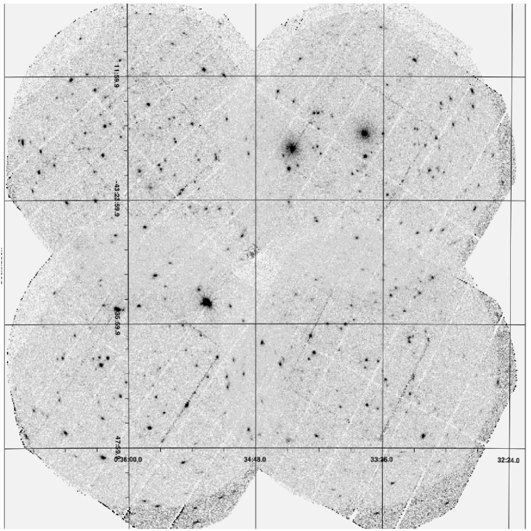
Figure 1: Mosaic of the four XMM-Newton pointings (ELAIS-S1-A, ELAIS-S1-B, ELAIS-S1-C, ELAIS-S1-D) obtained by adding up the images of the PN and MOS cameras in the energy range 0.5-10 keV. The image is exposure map corrected. A smoothing factor with $\sigma=1.5$ pixel (or 6”) was applied. Two out of the three brightest sources in the field are extended sources, which are presented in Section 2.5; the other one is a type 1 AGN at z$=$0.143 (La Franca et al. 2004).

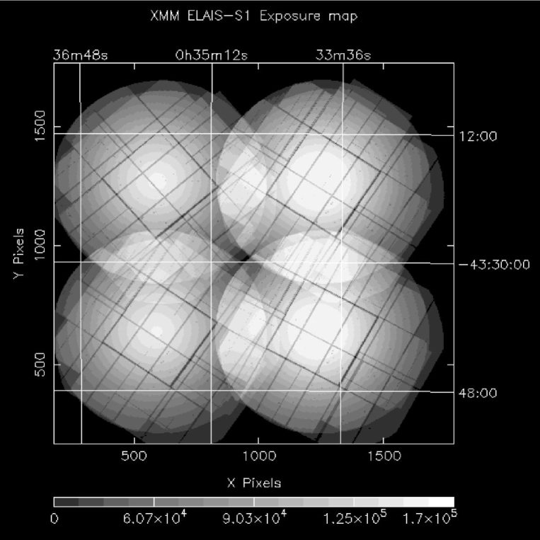
Figure 2: 0.5-10 keV exposure map of the mosaic of the four XMM-Newton pointings (ELAIS-S1-A, ELAIS-S1-B, ELAIS-S1-C, ELAIS-S1-D), obtained by adding to the PN exposure map, the MOS exposure maps weighted on the relative effective area.

2.2 Source detection

Source detection was performed on coadded (in sky coordinates) PN+MOS1+MOS2 images accumulated in four energy bands: 0.5-10 keV (full band, F), 0.5-2 keV (soft band, S), 2-10 keV (hard band, H), 5-10 keV (ultra hard band, HH). These bands have been chosen to ease the comparison with previous work. The EPIC effective area strongly decreases after 4-5 keV and therefore the 2-10 keV count rate is dominated by the count rate at the lower end of the band, unless the spectrum is extremely hard and/or heavily absorbed. At the flux limit of our survey we expect that only a minority of the 2-10 keV sources are highly obscured (see Comastri et al. 2001). In fact, the number of sources detected in the 2-10 keV band is similar (within 10 %) to the number of sources detected in the 2-5 keV band.

The source detections and the X-ray photometry were perfomed by using the PWXDetect code, developed at INAF - Osservatorio Astronomico di Palermo, following Pillitteri et al. (2006). The code is derived from the original ROSAT code for source detection by Damiani et al. (1997) and allows one to combine data from different EPIC cameras and data taken in different observations, in order to achieve the deepest sensitivity. The code is based on the analysis of the wavelet transform (WT) of the count rate image. A WT of a two-dimensional image is a convolution of the image with a “generating wavelet” kernel, which depends on position and length scale. In the algorithm developed by Damiani et al. (1997), the generating wavelet is a “mexican hat”. The length scale is a free parameter; therefore this method is particularly well suited for the cases in which the point-spread function (PSF) is varying across the image. It also provides robust detections of extended sources.

As a first step, a preliminary background map is computed by a suitable smoothing of the image and using also exposure maps to handle spatial exposure non-uniformities. Then, a local median filter is applied to recompute the background at several scales, to minimize the effect of point sources on the background determination. The WT algorithm is applied at several wavelet scales. Spatial maxima are selected if their heights are above the expected background at a chosen significant level. Information about position, shape and count rate of the sources are retained for the detection scale at which each source has the maximum significance. The background is then recomputed, excluding sources found at the first step and WT procedure is repeated in order to detect the weakest sources. The final source list with their positions, detection scales and photometry is then built. We have chosen a significance level corresponding to a probability of 2$\times$10^-5 that a maximum is a Poisson fluctuations of the background. This corresponds to about one spurious source per field. To calibrate this probability we performed 150 simulations of each field in each energy range, assuming a background equal to the total counts in each field (see last column of Table 1). We then applied the WT algorithm to each simulation and evaluated the significance level for which we have one spurious source per field.

To evaluate count rates, we have chosen PN as the reference detector. The scaling factor (r) between PN, MOS1 and MOS2 depends on the relative instrument efficiency and source spectral shape. We evalued this factor for each energy band, from the PN, MOS1, MOS2 count rate ratios, predicted for a power law model with an energy index $\alpha_{E}=0.8$. The count rates in the summed image (CR_Sum) are equivalent to PN count rates according to the following formula:

$$\mathrm{CR_{Sum}}=\mathrm{CR}_{\mathrm{PN}}+\mathrm{CR}_{\mathrm{MOS1}}\cdot r_{\mathrm{MOS1/PN}}+\mathrm{CR}_{\mathrm{MOS2}}\cdot r_{\mathrm{MOS2/PN}}$$

where the scaling factors $r_{\mathrm{MOS1/PN}}$ and $r_{\mathrm{MOS2/PN}}$ are similar. The exposure times used to calculate the count rates are obtained from exposure maps, and thus they take into account all spatial non-uniformities due to vignetting, chip geometry, CCD gaps. We have checked that the source count rates evalued by the PWXDetect, are consistent with the count rates in single PN and MOS cameras.

448 sources are detected in the F band images with a probability lower than 2$\times$10^-5 that they are Poisson background fluctuations, the weakest sources having at least 10 net counts in each EPIC cameras (see Table 2 for more details). The signal to noise ratio of the weakest detections in the coadded PN+MOS1+MOS2 images is $\sim 3$ . 395, 205 and 31 sources are detected in the coadded S, H and HH band images respectively (see Table 3 for more detail). Seven of the detected sources are clearly extended. We discuss these sources in Sect. 2.5. The quality of the detections and of the X-ray centroids were always checked interactively. We further checked the quality of the WT algorithm detections by comparing the distributions of the source counts, count rates, background, signal to noise ratio, and probability to that obtained using the SAS maximum likelihood method on the XMM-Newton survey of the COSMOS field (Cappelluti et al., in preparation), obtaining consistent results.

The source catalog, including position and fluxes, will be electronically available from VizieR. It is available also at the following site: http://www.mporzio.astro.it/ELAIS-S1. This site gives access to a multiwavelenth catalog which also includes optical, near infrared and mid infrared magnitudes and fluxes and optical spectroscopy. The optical follow-up campaign is currently on going and therefore the multiwavelength catalog cannot be part of this publication and will be properly presented in a future paper (Feruglio et al., in preparation).

Table 2: Sources detected in each of the XMM-ELAIS-S1 field

Energy range	PN counts a	MOS counts b	Nc
ELAIS-S1-A
0.5-10 keV	10-450	10-350	152
0.5-2 keV	15-370	20-250	135
2-10 keV	10-110	10-110	73
5-10 keV	25-30	20-25	13
ELAIS-S1-B
0.5-10 keV	15-5700	15-7000	106
0.5-2 keV	15-5100	20-5800	102
2-10 keV	10-600	10-1100	62
5-10 keV	10-100	10-140	8
ELAIS-S1-C
0.5-10 keV	15-590	20-450	157
0.5-2 keV	10-1000	10-830	134
2-10 keV	20-190	15-140	69
5-10 keV	15-40	5-20	11
ELAIS-S1-D
0.5-10 keV	20-420	20-300	126
0.5-2 keV	10-350	15-260	112
2-10 keV	15-130	15-80	54
5-10 keV	10-35	10-35	7

Minimum-maximum net counts of the detected sources in the PN camera (^a), and MOS1$+$MOS2 cameras (^b). The counts are not corrected for vignetting and PSF. (^c) Number of the detected sources in each of the four energy bands and in each field. Note that the four XMM-Newton pointings are partially overlapping, therefore the sum of the sources in this table is larger than the total number of the detected sources; note also that the brightest source in the ELAIS-S1-B field lies close to a gap between two PN CCDs.

Table 3: Detected sources

X-ray bands	Na
S	395
H	205
HH	31
F	448
F+S+H+HH	27
F+H+HH	1
F+S+HH	3
F+S+H	140
F+H	33
H only	4
F+S	199
F only	45
S only	26

^a Number of detected sources.

2.3 Count rates, fluxes and sky-coverage

Source count rates in the four bands were extracted and corrected for the energy dependent vignetting (as calibrated in orbit by Lumb et al. (2003)) and PSF (using the analytical approximation given by Ghizzardi (2001) and Ghizzardi (2002)). The PN and MOS 4 keV PSF half power diameter (HPD) is $\sim$20 and $\sim$16 arcsec, respectively, at small ($<$2 arcmin) off-axis angles; it increases only by a few $\%$ at off-axis angles of 10 arcmin. Even at these large off-axis angles, the core can be safely considered axis-symmetric.

For a sample of 40 sources in a broad range of brightness and off-axis angles, we compared the count rates evaluated using the WT algorithm to the count rates measured from spectra extracted from 35$-$40 arcsec radius regions. The count rates measured from spectra were corrected for the telescope vignetting and PSF. We found that the count rates obtained using the WT algorithm are  $\sim$8$\%$ and  $\sim$4$\%$ lower than the count rates measured from the spectra in the F band and S band respectively. We then corrected the count rates evaluated using the WT algorithm by these amounts. The weighted mean of the best fit spectral indices is $\alpha_{E}=0.8\pm 0.2$ ($1\sigma$ confidence level).

Count rates were converted to fluxes using the following conversion factors: 1.6$\times 10^{-12}$ ${\rm erg\leavevmode\nobreak\ cm}^{-2}\leavevmode\nobreak\ {\rm s}^{-1}$ (S band), 8.3$\times 10^{-12}$ ${\rm erg\leavevmode\nobreak\ cm}^{-2}\leavevmode\nobreak\ {\rm s}^{-1}$ (H band) and 16.5$\times 10^{-12}$ ${\rm erg\leavevmode\nobreak\ cm}^{-2}\leavevmode\nobreak\ {\rm s}^{-1}$ (HH band), which are appropriate for a power law spectrum with energy index $\alpha_{E}=0.8$. These three conversion factors are not strongly sensitive to the spectral shape, due to the narrow bands: for $\alpha_{E}=0.4$ and 1.0 they change by up to $\sim 1\%$ in the S band and by up to 10% in the H band. For an absorbed power law spectrum with $N_{H}=10^{22}$ cm^-2 and $\alpha_{E}=1$ the conversion factors change by $<1\%$ in the H band and by $\sim 14\%$ in the S band. The conversion factor for the F band depends more on the spectral shape because of the wider band. For a power law spectrum with $\alpha_{E}=0.8\pm_{0.4}^{0.2}$ it changes by up to $30\%$. To minimize this error, we therefore decided to follow a different approach for the F band: we used a variable conversion factor which is a function of the spectral shape, estimated from the hardness ratios (H-S)/(H+S). The histogram of the number of sources as a function of the flux is given in Figure 3. We detect sources in the 0.5-2 keV and 2-10 keV bands down to flux limits of $\sim 5.5\times 10^{-16}$ ${\rm erg\leavevmode\nobreak\ cm}^{-2}\leavevmode\nobreak\ {\rm s}^{-1}$ and $\sim 2\times 10^{-15}$ ${\rm erg\leavevmode\nobreak\ cm}^{-2}\leavevmode\nobreak\ {\rm s}^{-1}$ respectively.

Figure 3: The distribution of the detected sources as a function of the flux in the 0.5-2 keV band (solid line, empty histogram), 2-10 keV band (shaded histogram) and 5-10 keV band (black histogram).

The “Sky coverage” defines the area of the sky covered down to a given flux limit, as a function of the flux. Due to the telescope vignetting and to the increase of the size of the PSF in the outer regions of the detector, the sensitivity decreases toward the outer detector regions.

The minimum number of counts needed to exceed the Poisson fluctuations of the background, with a probability threshold of 2$\times$10^-5 in each detector position has been evaluated using the background maps in each band and the PSF shape as a function of the off-axis angle. This minimum number of counts has been divided by the exposure map and thus converted to minimum detectable fluxes (limiting flux) using the above defined count rate–flux conversion factors for the S, H and HH bands. The F band limiting count rates were converted to fluxes using a conversion factor of 3.25$\times 10^{-12}$ ${\rm erg\leavevmode\nobreak\ cm}^{-2}\leavevmode\nobreak\ {\rm s}^{-1}$ , which is appropriate for a power law spectrum with $\alpha_{E}=0.8$. The sky coverage at a given flux is then obtained by adding up the contribution of all detector regions with a given flux limit. Figure 4 plots the resulting sky-coverage in the four bands. In each band the sky coverage curve is very steep near the faintest detectable flux, typically decreasing by an order of magnitude for a change in the limiting flux of $\sim 10\%$.

Figure 4: The sky coverage in the four 0.5-10 keV, 0.5-2 keV, 2-10 keV and 5-10 keV bands. The count rate–flux conversion factors are appropriate for a power law spectrum with $\alpha_{E}=0.8$.

The main sky coverage uncertainty is due to the unknown spectrum of the sources near the detection limit. Of course, this uncertainty increases with the width of the band and therefore is largest in the F band. To estimate, at least roughly, this uncertainty, we calculated the sky coverage also for power law spectra with $\alpha_{E}=0.4$, $\alpha_{E}=1.0$, and for absorbed power law spectra with $\alpha_{E}=0.4,1.0$ and N${}_{H}=10^{22}$ cm^-2, in addition to the baseline case. At fluxes higher than a few $\times 10^{-14}$ ${\rm erg\leavevmode\nobreak\ cm}^{-2}\leavevmode\nobreak\ {\rm s}^{-1}$ the percentage deviations of the sky coverage with respect to the baseline case are negligible for all energy bands. At a flux of $10^{-14}$ ${\rm erg\leavevmode\nobreak\ cm}^{-2}\leavevmode\nobreak\ {\rm s}^{-1}$ the deviations are $\sim 75\%$ in the F band, $\sim 30\%$ in the H band and negligible for the other bands. At a flux of $5\times 10^{-15}$ ${\rm erg\leavevmode\nobreak\ cm}^{-2}\leavevmode\nobreak\ {\rm s}^{-1}$ the deviations are $\sim 100\%$ in the F band, $\sim 80\%$ in the H band and negligible in the S and HH bands.

2.4 Source confusion

Source confusion can affect at some level deep XMM-Newton images. At 0.5-2 keV and 2-10 keV fluxes of $1.5\times 10^{-15}$ ${\rm erg\leavevmode\nobreak\ cm}^{-2}\leavevmode\nobreak\ {\rm s}^{-1}$ , and $5\times 10^{-15}$ ${\rm erg\leavevmode\nobreak\ cm}^{-2}\leavevmode\nobreak\ {\rm s}^{-1}$ , corresponding to a sky coverage of $\sim$0.04 square degrees, we expect $\sim 750-600$ sources deg^-2, using the number counts from the compilation of Moretti et al. (2003). The probability of finding two sources with the above fluxes within 12” arcsec from each other (twice the size of the typical detection cell) is only $\sim 2-2.5\%$ for the S and H bands, respectively. These probabilities go up to $\sim(4-5)\%$ for fluxes corresponding to the faintest detected sources in the two bands. The spatial extension and asymmetry in the count distribution of the sources were checked interactively, to understand whether same of the X–ray sources can actually result from the blend of two or more sources. We find that this may be the case for $\sim 14$ sources (i.e., 3% of the whole F sample) at fluxes ${{}_{<}\atop{}^{\sim}}3\times 10^{-14}$ ${\rm erg\leavevmode\nobreak\ cm}^{-2}\leavevmode\nobreak\ {\rm s}^{-1}$ and for 2 sources at fluxes $\sim 1.4\times 10^{-13}$ ${\rm erg\leavevmode\nobreak\ cm}^{-2}\leavevmode\nobreak\ {\rm s}^{-1}$ . Nine of these sources have been deblended and their count rates has been measured interactively from the images. The remaining 7 sources have morphologies and surface brightnesses typical of extended sources (2 of them are bright clusters of galaxies, see Sect. 2.5). We conclude that source confusion does not significantly affect our results, especially the X-ray number counts presented in Sect. 3.

2.5 Extended sources

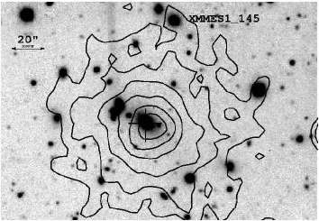
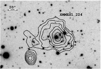
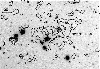
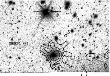
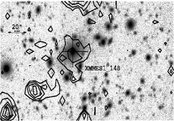
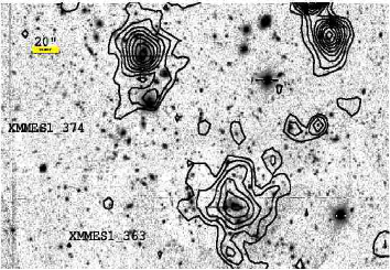
Figure 5: 0.5-10 keV contours of the seven extended sources overlayed on the R band VIMOS images (XMMES1_145, XMMES1_224 and XMMES1_184, XMMES1_444, XMMES1_374, XMMES1_363,XMMES1_148). The crosses indicate the brightest galaxy associated with each cluster.

Table 4: Extended sources, X-ray data

Source name	R.A.	DEC.	PNa	MOSb	F(0.5-10keV)	KT	z	logLX
	J2000	J2000	net counts	net counts	$10^{-14}$ c.g.s.	keV		erg s-1
XMMES1_145	8.44298	-43.29217	3228$\pm$74	2713$\pm$68	14.6	2.7$\pm$0.2	0.21$\pm$0.01	43.3
XMMES1_148	8.44469	-43.34471	134$\pm$16	105$\pm$17	0.6	1.8$\pm_{0.4}^{0.8}$	0.27$\pm_{0.08}^{0.14}$	42.2
XMMES1_184	8.52914	-43.37431	203$\pm$25	155$\pm$22	0.8	1.3$\pm$0.2	0.4$\pm_{0.1}^{1.3}$	42.8
XMMES1_224	8.61410	-43.31646	2448$\pm$58	1865$\pm$51	14.3	3.2$\pm$0.3	0.39$\pm$0.02	43.9
XMMES1_363	8.94811	-43.38005	303$\pm$25	261$\pm$23	1.6	2.7$\pm_{0.5}^{0.7}$	1.10$\pm$0.13	44.1
XMMES1_374	8.97218	-43.35345	283$\pm$24	224$\pm$22	1.2	1.1$\pm$0.1	0.37$\pm$0.06	42.7
XMMES1_444	9.11833	-43.47706	201$\pm$22	176$\pm$20	2.5	3.1$\pm_{1.1}^{2.5}$	0.7$\pm_{0.4}^{3.3}$	43.7

^aNet PN counts in the 0.5-10 keV energy range. ^bNet MOS1+MOS2 counts in the 0.3-10 keV energy range. The quoted errors corresponds to 68% confidence level.

Table 5: Extended sources: optical and near infrared data¹ of the brightest galaxy associated with each cluster.

Source name	R.A.	DEC.	B	V	R	K	J	zphot
	J2000	J2000	mag	mag	mag	mag	mag
XMMES1_145	8.4433322	-43.291992	19.24	17.76	16.99	13.86	15.15	0.15-0.30
XMMES1_148	8.4452075	-43.344633	20.07	18.54	17.74	14.57	15.90	0.15-0.75
XMMES1_184	8.5332721	-43.377095	20.79	19.31	18.25	14.59	16.13	0.25-0.80
XMMES1_224	8.6080313	-43.314348	20.79	19.19	17.93	14.36	14.55	0.25-0.85
XMMES1_363	8.948075	-43.379401	23.31	21.34	20.21	16.13	17.48	0.65-0.95
XMMES1_374	8.9731188	-43.353933	22.23	20.56	19.47	16.07	17.41	0.25-0.80
XMMES1_444	9.1195568	-43.475508	21.07	19.44	18.24	14.63	16.30	0.30-0.80

¹ Magnitude in the Johson-Cousins Vega system.

Figure 6: Radial distribution of the background subtracted surface brightness, normalized to the peak central value, of the sources XMMES1_145, XMMES1_148, XMMES1_184, XMMES1_224, XMMES1_363, XMMES1_374 and XMMES1_444, computed in concentric annuli (full dots), compared that of point–like sources at the same off-axis angles (open dots).

We identified seven extended X-ray sources by comparing their background subtracted surface brightness, computed in concentric annuli, to the background subtracted surface brightness of point-like sources found at similar off-axis angles, which provide a reasonably good representation of the local PSF. The surface brightness radial profiles of these sources, normalized to the peak surface brightness are shown in Figure 6. For all of them, the difference with the radial profiles of the point-like sources are significant at more than 99.9%.

Figure 5 shows the X-ray contours of the 7 sources overlayed on deep R band optical images obtained using VIMOS@VLT ESO telescope. We see that all sources can be identified with clusters or groups of galaxies.

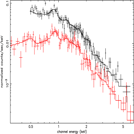
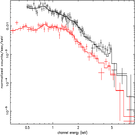
Figure 7: PN and MOS counts spectra of the two brighest extended sources, XMMES1_145 (left panel) and XMMES1_224 (right panel), along with their best fit thermal models.

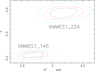
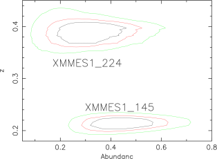
Figure 8: Left panel: the 68%, 90% and 99% redshift-temperature $\chi^{2}$ contours for the two clusters of galaxies XMMES1_145 and XMMES1_224. Right panel: The 68%, 90% and 99% redshift-metal abundance $\chi^{2}$ contours.

We extracted the X-ray spectra of the 7 extended sources from circular regions with radii in the range 35$\arcsec$ to 70$\arcsec$. The background counts were extracted from the nearby source-free regions. The response and ancillary files were generated by the XMM-SAS tasks, rmfgen and arfgen, respectively. The MOS1 and MOS2 spectra are combined together. The spectra were fitted using XSPEC (version 11.3.1, Arnaud (2003)), to a thin plasma thermal model with free temperature and redshift. For the two brightest sources (XMMES1_145 and XMMES1_224, see Table 4), the statistics is good enough to let also the metal abundance to be free to vary in the fit. Figure 7 shows the PN and MOS spectra of these two sources along with the best fit thermal model. In the other five cases, we fixed the metal abundance to the typical value (0.3) found in clusters of galaxies over broad redshift range (see, e.g., Tozzi et al. (2003)). Table 4 gives for each of the extended sources the X-ray position, the net counts in the 0.5-10 keV energy range and the corresponding flux, the best fit temperature, redshift and X–ray luminosity.

Figure 8 shows the temperature-redshift and redshift-metal abundance $\chi^{2}$ confidence contours for the sources XMMES1_145 and XMMES1_224. The quality of the XMM-Newton data is such to tightly constrain the redshift of the two bright clusters (0.21$\pm$0.01 and 0.39$\pm$0.02). Figure 9 shows the temperature-redshift $\chi^{2}$ contours for the sources XMMES1_374, XMMES1_363, XMMES1_184 and XMMES1_148. Although in these cases the statistics is limited (see counts and fluxes in Table 4) the XMM-Newton data are still good enough to provide rough information on the redshift of the sources. Note that the redshift of XMMES1_363 is constrained to be $>0.7$ at the 90% confidence level, and that 4 of the sources ( XMMES1_224, XMMES1_374, XMMES1_184 and XMMES1_148) are consistent with having the same redshift (z$\sim$0.4). The luminosities and temperatures in Table 4, both determined through the X-ray spectral fittings, are in good agreement with the luminosity-temperature relationship of groups and clusters of galaxies (see, e.g., Arnaud (2005) and references therein).

Table 5 gives the position and the B, V, R, K and J magnitudes of the brightest galaxies of each of the seven X-ray sources in Figure 5. We estimated their photometric redshifts by comparing the observed optical to near infrared spectral energy distribution with the Rocca-Volmerage galaxy templates (see, e.g., Fioc & Rocca-Volmerage 1997). Unfortunately, the available photometry does not allow a precise determination of the redshifts of the galaxies, but the redshift confidence intervals in Table 5 are in all cases consistent with the redshift estimates in Table 4. In particular, the photometric redshifts confirm that XMMES1_363 is at a redshift higher than the rest of the extended sources sample.

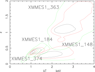
Figure 9: The 68%, 90% and 99% redshift-temperature $\chi^{2}$ contours for the sources XMMES1_148, XMMES1_184, XMMES1_363 and XMMES1_374.

3 The X-ray number counts

The XMM-Newton survey in the ELAIS-S1 area covers a range of fluxes over an area which is large enough to constrain source counts in a flux range bridging deep, pencil beam, and shallower, large area surveys. Figure 10 plots the integral number counts in the F, S, H and HH bands. Table 6 gives the number counts in the S, H and HH bands, which can be more easily compared with previous determinations, together with the sky coverage in the same bands. Previous determinations of the S, H and HH number counts are over-plotted on the ELAIS-S1 number counts. The 0.5-2 keV number counts are compared to those of Rosati et al. (2002) (Chandra Deep Field South, CDFS), Moretti et al. (2003) (compilation), Baldi et al. (2002) (HELLAS2XMM) and Hasinger et al. (2005) (compilation). The CDFS number counts are the lowest, as already noted by Rosati et al. (2002). The ELAIS-S1 determination is consistent within the errors with those of Moretti et al. (2003) and Baldi et al. (2002). The ELAIS-S1 2-10 keV number counts are compared to those of Rosati et al. (2002), Moretti et al. (2003), Baldi et al. (2002) and Giommi et al. (2000) (BeppoSAX). All determinations are consistent with each others at fluxes lower than $2-3\times 10^{-14}$ ${\rm erg\leavevmode\nobreak\ cm}^{-2}\leavevmode\nobreak\ {\rm s}^{-1}$ . The ELAIS-S1 5-10 keV number counts are compared to the those of Rosati et al. (2002), Hasinger et al. (2001) (Lockman Hole), Baldi et al. (2002) and Fiore et al. (2001) (BeppoSAX). The ELAIS-S1 number counts are slightly lower than the other determinations but still consistent within the errors. In summary, the agreement of the ELAIS-S1 number counts with other determinations is reasonably good, implying that the ELAIS-S1 region, at least from this point of view, can be considered as representative of the average X-ray source population.

Table 6: Integral number counts and sky coverage

Flux	N1	Counts	Sky-coverage
$10^{-14}$ ${\rm erg\leavevmode\nobreak\ cm}^{-2}\leavevmode\nobreak\ {\rm s}^{-1}$		deg-2	deg2
0.5-2 keV
0.10	23	854$\pm$60	0.03
0.15	50	564$\pm$31	0.38
0.23	61	473$\pm$27	0.57
0.36	84	321$\pm$22	0.62
0.55	59	223$\pm$19	0.63
0.83	48	138$\pm$15	0.64
1.30	30	75$\pm$11	0.64
1.99	23	33$\pm$7	0.64
3.04	5	11$\pm$4	0.64
4.55	4	5$\pm$3	0.64
7.15	1	3$\pm$2	0.64
11.00	1	2$\pm$2	0.64
2-10 keV
0.47	18	746$\pm$91	0.04
0.63	19	470$\pm$43	0.10
0.86	26	297$\pm$25	0.22
1.16	32	212$\pm$19	0.42
1.57	35	152$\pm$16	0.54
2.12	27	99$\pm$13	0.59
2.87	22	46$\pm$9	0.61
3.88	15	21$\pm$6	0.61
5.25	4	5$\pm$3	0.61
7.10	1	2$\pm$2	0.61
5-10 keV
0.69	3	156$\pm$47	0.013
0.96	4	91$\pm$24	0.07
1.34	3	51$\pm$12	0.17
1.86	7	35$\pm$9	0.31
2.59	11	15$\pm$5	0.45
3.60	1	2$\pm$2	0.52

¹ Detected sources per flux bin. Note that a few sources fall out of the flux range, which was used to evalued the integral number counts in each energy band.

Figure 10: The source number counts in the 0.5-10 keV F band (upper left panel), 0.5-2 keV S band (upper right panel), 2-10 keV H band (lower left panel), 5-10 keV HH band (lower right panel). The Figure also shows a few number counts from literature: the 0.5-2 keV number counts from Rosati et al. (2002), Moretti et al. (2003), Baldi et al. (2002) and Hasinger et al. 2005 (upper right panel); the 2-10 keV number from Rosati et al. (2002), Moretti et al. (2003), Baldi et al. (2002) and Giommi et al. (2000) (lower left panel); the 5-10 keV number from Rosati et al. (2002), Hasinger et al. (2001), Baldi et al. (2002) and Fiore et al. (2001) (lower right panel).

4 X-ray spectral properties

Figure 11: Left panel: The hardness ratio (H-S)/(H+S) as a function of the flux for the whole 2-10 keV sample. Typical hardness ratio errors are shown at different fluxes. 1$\sigma$ upper limits on the S band flux are shown with by arrows. Large filled circles represent the median and interquartile in two flux ranges, evalued using the so called “survival analysis”(Kaplan and Meier, (1958), Miller 1981, p. (74)). They are compared with the same determination from the HELLAS2XMM sample (open squares). Constant lines are the hardness ratios expected from a power law model with slope $\alpha=$0.8, reduced at low energy by photoelectric absorption from neutral gas (N_H$=$ 10²² cm^-2 and 10²³ cm^-2) at three representative redshifts: z=0, z=1 and z=2. Right panel: The distribution of (H-S)/(H+S) for the same sample in the left panel (solid histogram). Upper limits are identified by the shaded histogram. The dotted histogram is the average of the simulated (H-S)/(H+S) distributions.

Figure 12: The source number counts in the F band (upper left panel), S band (upper right panel), H band (lower left panel), HH band (lower right panel). The open circles indicate the source number counts of the unobscured sources. The solid circles indicate the source number counts of the obscured sources, as defined in Sect. 4.

The broad band X-ray spectral properties of the ELAIS-S1 sources can be investigated using hardness ratios. Many of the ELAIS-S1 sources have a high hardness ratio HR$=$(H-S)/(H+S) (where H and S are the fluxes in the hard and soft band, respectively, (see, e.g., Fiore et al. 2003)), indicating a hard spectrum. H-S/H+S for the full 2-10 keV sample, 205 sources, is plotted in Figure 11, left panel, as a function of the 2-10 keV flux. Lines of constant $N_{H}$ are overlaid. Following Hasinger et al. (2003) a threshold of the (H-S)/(H+S) ratio can be used to roughly separate obscured from unobscured sources. To this purpose we use HR=0.5, which corresponds to log N${}_{H}>21.5$, 22.2, 22.7 at z=0, 1, 2, respectively (assuming a power law slope $\alpha$=0.8).

According to this definition, the fraction of obscured sources to the total is 0.36. Of course, since errors on HR are large, especially at low fluxes, the separation between obscured and unobscured sources has only a statistical meaning. To evaluate how the fraction of the obscured sources is affected by the errors of HR, we generated 1000 random source distributions with the same number of sources as the real data, by assigning to each source a random HR value drawn from a gaussian distribution with mean equal to the measured HR and $\sigma$ equal the HR error. We then computed the dispersion of the number of sources with HR$>0.5$, which turned out to be about 5%. The dotted histogram in the right panel of Figure 11 is the average of the simulated (H-S)/(H+S) distributions. The last point of the simulated (H-S)/(H+S) distribution deviates from that of the real (H-S)/(H+S) distribution because the former takes properly into account the upper limits, which are plotted in the solid histogram at their nominal values.

Adopting the above definition, Figure 12 shows number counts of obscured and unobscured sources respectively, while Figure 13 shows the ratios between the number of the obscured sources to the total. The fraction of obscured sources increases with the energy of the X-ray band, consistently with Comastri et al. (2001). In the 2-10 keV band the fraction of obscured sources increases from  $\sim$20% at fluxes $>(4-5)\times 10^{-14}$ ${\rm erg\leavevmode\nobreak\ cm}^{-2}\leavevmode\nobreak\ {\rm s}^{-1}$ to $\sim 40\%$ at fluxes $\sim(1-2)\times 10^{-14}$ ${\rm erg\leavevmode\nobreak\ cm}^{-2}\leavevmode\nobreak\ {\rm s}^{-1}$ (consistent with Piconcelli et al. (2003), Ueda et al. (2003), Perola et al. (2004), La Franca et al. (2005)). It should be beared in mind that all this refers to moderately obscured sources only, since sources obscured by column densities N${}_{H}>$a few $10^{24}$ cm^-2, the so called Compton thick AGNs, are rarely detected even in 2-10 keV samples (see Tozzi et al. 2006).

Figure 13: Ratio between the number of the obscured sources to the number of the total sources in the S, H, HH bands (from top to bottom).

5 The angular correlation function

We now focus on the clustering properties of our X-ray sources. The fraction of active galaxies in our samples is probably higher than 80-90% in all bands (according to previous identification of X-ray sources at similar flux limits, see, e.g., Mainieri et al. 2002, Fiore et al. 2003, Barger et al. 2005). We computed the two point source angular correlation function (ACF, Peebles (1980)) in the three S, H and F bands using the Landy & Szalay (LS, 1993) estimator. The ACF function is given by the following relation:

$$w_{LS}(\theta)={k_{1}\times DD-2\times k_{2}\times DR+RR\over RR},$$

where $DD$ is the number of pairs of sources in the real data with separation angle in the interval $\theta,\,\theta+d\theta$, $RR$ is the number of pairs in the same separation angle interval using a spatially random distribution of sources, $DR$ is the number of pairs obtained comparing real data and random data, and $k_{1}={n_{r}(n_{r}-1)\over{n_{d}(n_{d}-1)}}$, $k_{2}={(n_{r}-1)\over{2\times n_{d}}}$, where n_d is the total number of real sources and n_r is the number of random sources.

To evaluate $w(\theta)$ we followed two different methods: (1) we generated 300 random source distributions with the same number of sources as the real data by convolving a random source distribution with the differential source number counts and with the appropriate sensitivity maps. We adopted a cut in flux for both the real source and random source distributions to exclude from the ACF analysis the 10% faintest sources in the samples. We then computed the ACFs according to eq. (1) for each random realization and in logarithmically spaced $\theta$ bins. The distribution of the 300 ACF values in each $\theta$ bin is in most cases reasonably well fitted by a gaussian distribution and therefore we computed the mean and the rms values in each $\theta$ bin. (2) we generated a single random source distribution using 100 times more sources than in the real samples. Also in this case, we adopted a cut in flux for both the real source and random source distributions to exclude from the ACF analysis the 10% faintest sources and computed the ACFs according to eq. (1). In this case errors were computed adopting the following formula  (from Landy & Szalay, 1993):

$$\delta(\theta)={(1+w(\theta))\over\sqrt{(DD})}$$

Figure 14 shows the ACF in the S and H bands computed in bins of log $\theta=0.075$ following the second method. The solid lines represent the best fit $w(\theta)=(\theta/\theta_{0})^{1-\gamma}-\omega_{\Omega}$ function to the ACF. The $\omega_{\Omega}$ factor has been introduced following Landy & Szalay (1993), Daddi et al. (2000) and Basikalos et al. (2004) to take into account the so called “integral constraint”. This results from the fact that the correlation function is evaluated in a limited area, while the ACF is normalized to zero over the full sky. According to Roche et al. (1999) this implies that the $w(\theta)$ computed using eq. (1) over-estimates the real $w(\theta)$ by a constant quantity $\omega_{\Omega}$$=(1/\theta_{0})^{1-\gamma}\times C$, where C has been estimated following again Roche et al. (1999). Fixing $\gamma$ to 1.8, as in Vikhlinin & Forman (1995), Basilakos et al. (2005) and D’Elia et al. (2005), produces the following best fit correlation angles: $\theta_{0}=5.2\pm 3.8$ arcsec, $\theta_{0}=12.8\pm 7.8$ and $\theta_{0}=7.5\pm 3.1$ arcsec in the S, H and F bands respectively (errors are at 1$\sigma$ confidence level). Letting $\gamma$ to vary of course increases the already large errors on $\theta_{0}$ but does not change their best fit values. In fact the best fit $\gamma$ turn out to be $1.7^{+0.1}_{-0.5}$ and $1.8^{+0.1}_{-0.2}$ for the S and H bands respectively. To test the robustness of our determinations we computed the ACF with different bin sizes from log $\theta=0.05$ to log $\theta=0.1$. For the 0.5-2 keV ACF we found best fit $\theta_{0}$ in the range $\sim$4-9 arcsec, while for the 2-10 keV ACF we found best fit values in the range $\sim$9-19 arcsec. In all cases the best fit $\theta_{0}$ were consistent, within the errors, with the values given above.

Very similar results are obtained by using the first method to compute the $w(\theta)$ and the corresponding errors.

Since the correlation angles we probe are of the same order of magnitude of the XMM-Newton PSF, the so called amplification bias (see, e.g., Vikhlinin & Forman 1995) could in principle affect our estimates of w($\theta$) at small separations, due to sources closer than a few arcsec being observed as a single source. However, we note that at our limiting flux the source confusion affects our images little (see Sect. 2.5). Furthermore, since our fits have been performed on angular scales $\theta>100\arcsec$, much greater than the XMM-Newton PSF, the amplification bias is not expected to affect our estimates of the ACF. Indeed, Basilakos et al. (2005) found that amplification bias is negligible in their XMM-Newton 2dF survey.

Figure 14: The angular correlation function in the S band (top panel), and H band (bottom panel) computed using the Landy & Szalay estimator. The solid lines represent our best fit to the data between 100 and 1000 arcsec.

5.1 Source clustering

The ACF computed in the previous Sect. measures the strength of the angular correlation, but does not say anything about where the sources are clustered. To investigate this issue we plot in Figure 15a) and 15b) the source density map of the 0.5-2 keV and 2-10 keV sources, respectively, smoothed with a box of 10 arcmin side. The high density regions of both maps encompass the two clusters at z$\sim 0.4$ (XMMES1_224 and XMMES1_374) and other two clusters or groups of galaxies with a redshift consistent with 0.4. However, these observed source density maps are affected by instrumental biases, i.e. a higher source density is visible in the regions with the highest exposure (see Figure 2). To account for this effect, we computed the deviations of the real source distribution from a random source one, which has been obtained by convolving a random source distribution with the differential source number counts and with the appropriate sensitivity maps. We plot in Figure 15 c) and 15 d) the normalized source density $NNSD$ of the 0.5-2 keV and 2-10 keV sources respectively using the following equation:

$$NNSD(X,Y)=(NSD(X,Y)-NRD(X,Y))/NRD(X,Y)$$

where $NSD$ is the real source density and NRD is the density of a random source sample. The resulting normalized source density map has then been smoothed with a box of 10 arcmin side. The high density regions of the 0.5-2 keV map still encompass the four extended sources clusters at z$\sim 0.4$. On the other hand, the highest density region of the 2-10 keV map is just located in the central-west region of the field, in an area which coincides with one of the high density regions of the 0.5-2 keV map, but in which no extended source has been found.

6 Discussion

We have surveyed with XMM-Newton the central $\sim 0.6$ deg² region of the ELAIS-S1 field down to flux limits of $\sim 5.5\times 10^{-16}$ ${\rm erg\leavevmode\nobreak\ cm}^{-2}\leavevmode\nobreak\ {\rm s}^{-1}$ (0.5-2 keV), $\sim 2\times 10^{-15}$ ${\rm erg\leavevmode\nobreak\ cm}^{-2}\leavevmode\nobreak\ {\rm s}^{-1}$ (2-10 keV) and $\sim 4\times 10^{-15}$ ${\rm erg\leavevmode\nobreak\ cm}^{-2}\leavevmode\nobreak\ {\rm s}^{-1}$ (5-10 keV ). 448 sources have been detected in the 0.5-10 keV F band images with a probability lower than 2$\times$10^-5 that they are Poisson fluctuations of the background. 395, 205 and 31 sources are detected in the 0.5-2 keV, 2-10 keV and 5-10 keV band images respectively. Of these, 26 and 4 sources are detected only in the S and H band but not in the F band. The total number of detected sources is 478.

The source number counts are in good agreement with previous determinations from large area surveys and compilations (Baldi et al. 2002, Moretti et al. 2003), showing that field to field variance is smoothed out at the scale of the ELAIS-S1 survey (0.6 deg²) and implying that the ELAIS-S1 region, at least from this point of view, can be considered as representative of the average X-ray source population. The average spectral properties of the ELAIS-S1 sources are consistent with those of other surveys covering similar or larger areas at a similar depth. In particular, we find that: a) the fraction of obscured sources increases with the energy of the X-ray band and b) in the 2-10 keV band this fraction increases from  $\sim$20% at fluxes $>(4-5)\times 10^{-14}$ ${\rm erg\leavevmode\nobreak\ cm}^{-2}\leavevmode\nobreak\ {\rm s}^{-1}$ to $\sim 40\%$ at fluxes $\sim(1-2)\times 10^{-14}$ ${\rm erg\leavevmode\nobreak\ cm}^{-2}\leavevmode\nobreak\ {\rm s}^{-1}$ (consistent with Piconcelli et al. (2003), Ueda et al. (2003), Perola et al. (2004), La Franca et al. (2005)).

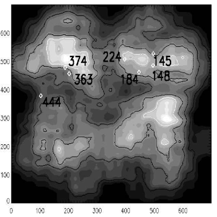
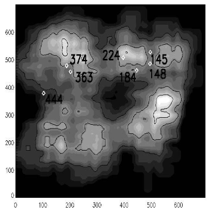
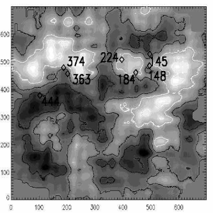
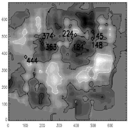
Figure 15: Top left panel a): the 0.5-2 keV source density contours, corresponding to -30%, -15%, 5%, 20% and 40% of the average source density; top right panel b): the 2-10 keV source density contours corresponding to -40%, -20%, 5%, 30% and 55% of the average source density. Darker regions correspond to underdensities and lighter regions to overdensities. The diamonds in all panels represent the 7 extended sources in the field (see Sect. 2.5). Bottom left panel c): same as top left panel for the normalized 0.5-2 keV source density; bottom right panel d): same as top right panel for the 2-10 keV source density contours.

We identified 7 clearly extended sources in the field and estimated their redshift through spectral fits with thermal models. In two cases the constraint on the redshift is quite accurate, $\sigma(z)/(1+z)<1.5\%$, in three other cases $\sigma(z)/(1+z)\sim(4-10)\%$, and in the remaining two cases the upper limit to the redshift is not well determined. Of course these uncertainties do not take into account possible systematic errors and should therefore be considered with some caution. The redshift of XMMES1_363 is constrained to be $>0.7$ at the 90% confidence level. In four cases (XMMES1_224, XMMES1_374, XMMES1_184 and XMMES1_148) the redshift is consistent with z$\sim$0.4. Photometric redshifts estimated using the B, V, R, K and J magnitudes of the brightest galaxies associated with the seven X-ray sources are all consistent with the redshifts estimated through their X-ray spectra. Interestingly, a peak at z$\sim 0.4$ is present in the spectroscopic redshift distribution of radio sources around XMMES1_374 and XMMES1_184 (Gruppioni et al. in preparation). The 0.5-10 keV luminosity of XMMES1_224 is $\sim 8\times 10^{43}$ erg s^-1, while the luminosity of the other three extended sources at a similar redshift is 15-60 times smaller. The angular separations between the luminous cluster XMMES1_224 and the 3 lower luminosity clusters or groups of galaxies are $5^{\prime}$ (XMMES1_184), $7.5^{\prime}$ (XMMES1_148) and $15.5^{\prime}$ (XMMES1_374), corresponding to 1.6, 2.4 and 5 Mpc at z$\sim$0.4, for the assumed cosmology. A detailed analysis of the extended sources and of the large scale structure at z$\sim 0.4$, including spectroscopic redshifts, will be presented in a forthcoming publication.

We have computed the angular correlation function of the sources in the S and H bands using the Landy & Szalay (1993) estimator. Fixing the slope of the correlation function at $\gamma=$1.8, we found the following correlation angles: $\theta_{0}=5.2\pm 3.8$ arcsec and $\theta_{0}=12.8\pm 7.8$ arcsec in the S, and H bands respectively, while the correlation angle in the 0.5-10 keV band is intermediate between these values. These estimates are fully consistent with the statistically poorer D’Elia et al. (2005) determinations. Basilakos et al. (2005) and Basilakos et al. (2004) found $\theta_{0}=10.4\pm 1.9$ arcsec in the S band and $\theta_{0}=28\pm 9$ in the H band for samples of sources of size similar to our ELAIS-S1 sample, but with a flux limit $\sim 5-6$ times higher than ours and spread over an area 4 times wider.

The correlation angle of hard X-ray selected sources is formally $\sim$2.5 times larger than that of soft X-ray selected sources (a correlation angle of hard sources higher than soft sources has been suggested also by Yang et al. 2003 and Basilakos et al 2004), although the difference is significant at only $\sim 1\sigma$ level. If real, this difference may be due to the different redshift distributions of hard and soft sources, because the angular correlation angle depends also on the average distance between galaxies, and therefore on their redshift. For a proper comparison one would need to evaluate the spatial correlation function, once the redshifts of the sources are known. A campaign to obtain optical spectroscopy of the optical counterparts of the X-ray sources is currently on going using VIMOS@VLT and the results will reported in a future publication. For the time being, we can obtain a rough estimate of the present-day correlation length r₀ assuming an appropriate redshift distribution dN/dz and inverting the Limber equation (Limber (1953), Peebles (1980)). We have estimated the observed redshift distributions of the S and H band sources, by convolving the best fit luminosity functions of La Franca et al. (2005, 2-10 keV) and Hasinger et al. (2005, 0.5-2 keV) with ELAIS-S1 sky coverage. Of course this approach does not take into account the presence of significant structures at a given redshift in the ELAIS-S1 field which could bias the redshift distribution of the ELAIS-S1 sources (one such structure may be present at z$\sim 0.4$, see Sect 2.5), and therefore the following results are should be considered as upper limits. Assuming an evolutionary parameter $\epsilon$ $=\gamma-3=-1.2$ (for $\gamma=1.8$, the so called “comoving clustering model”), which should be appropriate for active galaxies (Kundic (1997), Croom et al. (2001), Croom et al. (2005)), we obtain r${}_{0}=12.8^{+3.6}_{-5.7}$ h^-1 Mpc and r${}_{0}=17.9^{+4.2}_{-6.1}$ h^-1 Mpc in the S and H band respectively. So far we have obtained secure optical spectroscopy redshifts for 87 and 49 sources in the S and H bands (Feruglio et al., in preparation). Using these (admitedly incomplete) redshift distributions, which clearly shows strong peaks at z=0.4, we obtain r${}_{0}=9.8^{+2.7}_{-4.3}$ h^-1 Mpc and r${}_{0}=13.4^{+3.2}_{-4.6}$ h^-1 Mpc in the S and H band, respectively.

The S and H band redshift distributions are peaked at z$\sim$1 and z$\sim$0.9 respectively (median redshift) and therefore we are effectively measuring the clustering at those redshifts. The correlation length at a given redshift is: $r_{0}(z)=r_{0}\;(1+z)^{-{(3+\epsilon-\gamma)\over\gamma}}$, and therefore $r_{0}(z)=r_{0}$ for $\epsilon=-1.2$ and $\gamma=1.8$.

Our correlation lengths are lower but still consistent within the large errors with those of Basilakos et al. (2005) and Basilakos et al. (2004). On the other hand, for $\gamma=1.8$ Gilli et al. (2005) find r${}_{0}\sim$12 h^-1 Mpc and r${}_{0}\sim$6 h^-1 Mpc for the faint sources in the CDFS and CDFN fields respectively. The former estimate is consistent with our determination. We also note that although the median redshift of these sources is similar to the median redshift assumed above for the ELAIS-S1 sources, their fluxes (and therefore luminosities) are a factor of 5-10 lower than those of the sources in the ELAIS-S1 field. Yang et al. (2006) present a spatial correlation function analysis of the non-stellar X-ray point sources in the Chandra Large Area Synoptic X-ray Survey of Lockman Hole Northwest (CLASXS), covering a total area of 0.4 deg² down to a flux limit of 3$\times$10^-15 ${\rm erg\leavevmode\nobreak\ cm}^{-2}\leavevmode\nobreak\ {\rm s}^{-1}$ in the 2-8 keV band. They find r${}_{0}=8.1_{-2.2}^{+1.2}$ h^-1 Mpc, consistent with our determination obtained using the observed, but incomplete, redshift distributions.

We have also compared our correlation lengths to those obtained from optically selected QSOs, optically and near infrared selected galaxies and radio sources. Croom et al. (2005) find a low correlation length in redshift space $s_{0}=4.8\pm 1$ h^-1 for $\gamma=1.23$. Grazian et al. (2004) find a low $r_{0}=8.6\pm 2.0$ h^-1 Mpc for $\gamma=1.56$ and for a sample of local (0.02$<$z$<$0.22), optically selected AGN. Both determination are lower than our values. On the other hand, the correlation lengths of the ELAIS-S1 X-ray sources are comparable with that of Extremely Red Objects (EROs) (see, e.g., Daddi et al. 2001, r${}_{0}=12\pm 3$ h^-1 Mpc for $\gamma=1.8$ with 1$<$z$<$1.2) and luminous radio sources (see, e.g., Overzier et al. 2003, r${}_{0}=14\pm 3$ h^-1 Mpc for $\gamma=1.8$ ) at similar redshifts (z$\sim 1$).

We finally investigated whether the source density and clustering (on scales between 3 and 6 arcmin, where the signal in the ACF is more significant), are spatially related to the large scale structure discovered at z$\sim 0.4$. Figure 15 shows that there is a high normalized source density for the S band sample around the clusters and groups at z$\sim$0.4 (or with a redshift consistent with this value) extending both toward East and toward South/West, suggesting that the structure is complex, with a size comparable to the full XMM-Newton coverage. The highest normalized source densities of the H band sources are located in the South West and central-West regions of the field. The first is nearly coincident with one of the peaks of the S band source density, while the second has not a S band counterpart. The H band density peaks appear to be unrelated to the position of the extended sources at z$\sim 0.4$.

Sensitive observations over a wider area are clearly needed to both improve the statistics of the correlation functions and to cover several structures of the size of 10–20 Mpc in the same area, thus allowing us to understand whether these are peculiar structures, found by chance in selected areas of the sky, or whether, rather, they are representative of the average Large Scale Structure. The ongoing COSMOS multiwavelength survey will achieve these goals in the following years.