Abstract

We study how present data probe standard and non-standard properties of neutrinos and the possible existence of new light particles, freely-streaming or interacting, among themselves or with neutrinos. Our results include: $\sum m_{\nu}<0.40\,{\rm eV}$ at $99.9\%$ C.L.; that extra massless particles have abundance $\Delta N_{\nu}=2\pm 1$ if freely-streaming and $\Delta N_{\nu}=0\pm 1.3$ if interacting; that 3 interacting neutrinos are disfavored at about $4\sigma$. We investigate the robustness of our results by fitting different sub-sets of data. We developed our own cosmological computational tools, somewhat different from the standard ones.

1 Introduction

Thanks to recent data about the Cosmic Microwave Background (CMB), Large Scale Structures (LSS) and also Type Ia Supernovæ (SNe), cosmology has become the most sensitive probe of some neutrino properties (e.g. of neutrino masses: oscillation experiments test squared-mass differences, and other means of probing the absolute neutrino mass are currently less sensitive) and a very sensitive probe of other neutrino properties, including non standard ones [1, 2, 3]. In this paper we study how present cosmological data determine standard and non-standard ‘neutrino cosmology’. This includes three different issues.

• testing neutrinos: their masses, abundances, …

• do photons, neutrinos and gravitons make up the complete list of light particles? Data from particle physics allow extra light particles that are neutral under the Standard Model (SM) gauge group, and such extra light particles appear in many speculative extensions of the SM, one interesting example being simpler string models.

• The two above issues can be connected, because neutrinos are the least tested light particles and can easily interact with new light neutral particles, in a way that affects the evolution of cosmological inhomegeneities.

In section 2 we characterize the fundamental theories and describe the cosmological parameters that we want to extract from present data. Since our implementation of the cosmological computational tools needed for this analysis somewhat differs from the standard one, we describe it in section 3. Section 4 describes our results (table 1 might help in navigating the paper), summarized in the conclusions.

	Neutrino		Cosmology with extra light particles
	cosmology		freely-streaming		self-interacting		interacting with $\nu$
massless	$A_{s},n_{s},h$, $\Omega_{b},\Omega_{\rm DM},\tau$	§3	$\Delta N_{\nu}$	§4.2	$\Delta N_{\nu}$	§4.3	$N_{\nu},R\equiv{\displaystyle\frac{N_{\nu}^{\rm normal}}{N_{\nu}}}$	§4.6
massive	$\sum m_{\nu}$	§4.1	$\Delta N_{\nu},m_{\rm s}$	§4.4	$\Delta N_{\nu},m_{\rm s}$	§4.5	$R=0,m_{\nu}$ or $m_{\phi}$	§4.7,4.8

Table 1: Schematization of the cases considered in this paper. For each one we list the notation of the relevant parameters probed by cosmology and refer to the relevant part of the text.

2 Theory

The effects of new light particles on the evolution of cosmological inhomogeneities are often presented in terms of “non standard neutrino properties” because i) particle physics has tested neutrinos less thoroughly than other particles, leaving room for surprises; ii) neutrinos $\nu$ are the particles that can naturally interact with some new light neutral states. In this section, we discuss how established data and theory restrict the behavior of possible new light states, and in the rest of the paper we will consider scenarios that are compatible with these restrictions (more exotic possibilities are sometimes entertained in purely phenomenological analyses).

We consider light particles, neutral under all SM gauge interactions. Indeed the LEP measurement of the invisible $Z$ width [5] implies that hypothetical new light particles must be neutral under $\rm SU(2)_{L}$ gauge interactions and can have at most a small hypercharge; furthermore new light particles with strong interactions seem excluded. Field theory and gauge invariance significantly restrict the interactions of new neutral light particles in a well-known way that depends on their spin.

• New light fermions, neutral under all SM gauge interactions (commonly called ‘sterile neutrinos’ $\nu_{\rm s}$), can have a mass mixing with ordinary ‘active’ neutrinos. This is described by the following $\rm SU(2)_{L}\otimes{\rm U}(1)_{Y}$ gauge-invariant Lagrangian, written in compact notation

  $$\mathscr{L}(\nu_{\rm s})=\mathscr{L}_{\rm SM}+\bar{\nu}_{\rm s}i\partial/\hskip 1.29167pt\nu_{\rm s}+(\lambda LH\nu_{\rm S}+\frac{M}{2}\nu_{\rm s}^{2}+\hbox{h.c.}).$$ (1)

  $L$ and $H$ are the lepton and Higgs weak doublets.

• New light neutral scalars $\phi$ can have $\rm SU(2)_{L}\otimes{\rm U}(1)_{Y}$-invariant Yukawa interactions with sterile neutrinos, as described by the following Lagrangian:

  $$\mathscr{L}(\nu_{\rm s},\phi)=\mathscr{L}(\nu_{\rm s})+(\partial_{\mu}\phi)^{2}+(\frac{\lambda^{\prime}}{2}~{}\phi\,\nu_{\rm s}^{2}+\hbox{h.c.})+V(\phi).$$ (2)

  At energies below the mass of a sterile neutrino, it can be integrated out so that one effectively obtains Yukawa couplings $\nu\nu\phi$, suppressed by the mass of the sterile neutrino, as well as Yukawa couplings $\nu\nu_{\rm s}\phi$ with other lighter sterile neutrinos. We are aware of no reasonable allowed way of coupling a scalar directly to active neutrinos, in absence of light sterile neutrinos.

• Sizable couplings of neutrinos to light vectors can be introduced in a similar way: adding sterile neutrino(s) charged under an extra spontaneously broken gauge symmetry.

The gauge and Lorentz symmetries allowed theorists 30 years ago to successfully predict and guess experimental results. Theorists have tried to proceed further by demanding a further restriction: naturalness. At the moment it is unclear whether this is a correct requirement; for instance, the LHC will tell whether physics at the weak scale obeys it or not. Its imposition would strongly restrict the behavior of new light scalars. For example, one could explain their lightness by assuming that they are Goldstone bosons of spontaneously broken lepton numbers: in models with a single scalar, this implies that it couples to neutrino mass eigenstates (rather than to generic combinations), forbidding neutrino decay in vacuum.

Even taking into account that these considerations significantly restrict the set of ‘reasonable’ fundamental theories, flavour issues make the number of fundamental parameters so large that a direct study of the fundamental theory seems unpractical. (This approach has been pursued in [6] in the case of a single sterile neutrino and no bosons). On the other hand, cosmology probes (new) light particles via their gravitational couplings: neutrinos and new light particles affect the evolution of inhomogeneities in the gravitational potential(s), in which matter moves. Therefore it is convenient to focus on parameters half-way between theory and data: equation of state, sound speed, etc. We will consider the following basic limiting cases: extra freely-streaming particles, or extra particles that interact among themselves, or extra particles that interact with neutrinos. Whether a particular model falls in one or the other category depends on the value of the fundamental couplings (like $\lambda$, $\lambda^{\prime}$ and the interactions in $V(\phi)$ above) of the particular model.

In the following analyses we will study different systems specifying the parameters probed by cosmology. Some of these parameters will be combinations of the parameters appearing in the low-energy effective Lagrangian, some others will not (e.g. the abundances around recombination). The latters could be translated in terms of the fundamental parameters of each full model, a step that we do not make.

We ignore other possible probes of the same physics (which e.g. also manifests as neutrino decay, anomalous matter effects, rare $K\to\ell\nu$ decays), as they presently are orders of magnitude less sensitive than cosmology.

	‘Typical’ analyses	This analysis
Cosmological code	public CMBfast	our code
Language	FORTRAN	Mathematica
Statistics	Monte Carlo Markov chains	Gaussian

Table 2: Differences between our approach and a ‘typical’ cosmological analysis.

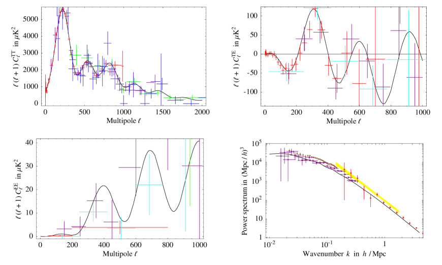
Figure 1: Our computation of CMB and LSS spectra in standard $\Lambda$CDM cosmology, compared with data.

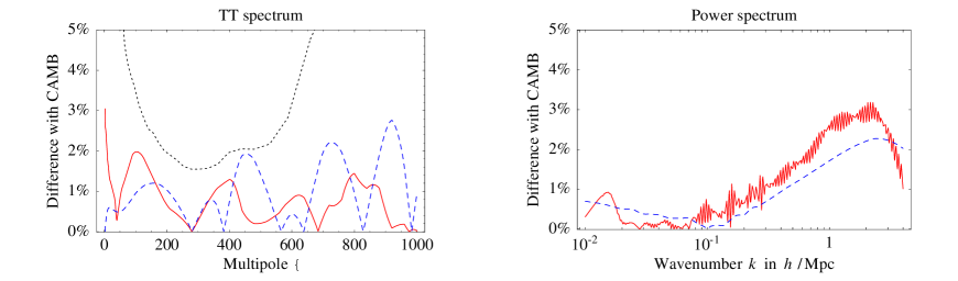
Figure 2: Difference between our code and CAMB, at the standard-cosmology best-fit point for $m_{\nu}=0$ (red solid line) and for $m_{\nu}=0.5\,{\rm eV}$ (blue dashed line). Our code does not employ any approximation specific for standard cosmology. In both codes various parameters allow the user to increase the accuracy; this plot holds for the choice employed in the present paper. The dotted line shows the $1\sigma$ accuracy obtained by WMAP3 results (binned data), indicating that we have a good enough accuracy (as confirmed by other tests). A similar $\%$-level accuracy is found for the TE and EE CMB spectra, that presently are measured with much larger uncertainties than the TT spectrum.

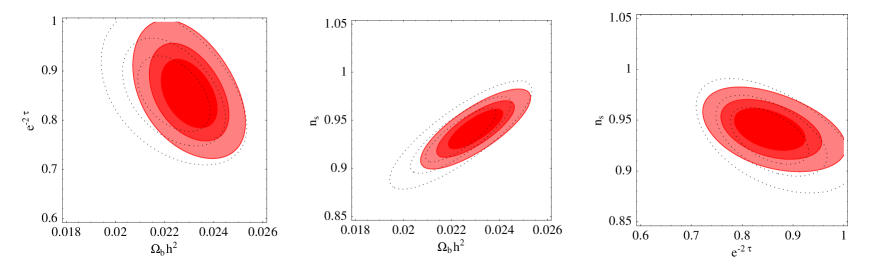
Figure 3: Fit of cosmological data at 68, 90 and 99% C.L. The shaded areas show our global fit without Lyman-$\alpha$, and the dotted lines our WMAP3-only fit, such that this figure can be directly compared with the analogous WMAP Science Team plots in fig. 10 of [7].

3 Analysis strategy

We develop our own computational tools for the analysis of the cosmological observables. For what concerns standard cosmology, our results agree with those of other authors (e.g. the WMAP Science Team), but having independent analyses is clearly important. In this respect, our analysis is particularly independent: it differs from what nowadays is a typical analysis in the way illustrated in table 2. Cosmological observables are computed using a code written by one of us, rather than running the commonly used CMBfast or CAMB public codes [8]: this allows us to have a better control and flexibility on non-standard modifications.

We use the line-of-sight approach in the conformal Newtonian gauge [8, 9, 10]; recombination can be implemented both in Peebles approximation (see e.g. [31]) and using the external recfast code [11], which is the option chosen for the present analysis.

The main disadvantage is that our code is almost $2$ orders of magnitude slower than CMBfast or CAMB. In part this happens because, rather than optimizing our code for standard cosmology, we keep it fully flexible such that non-standard cosmologies are immediately implemented. In part this happens because, while standard codes are written in FORTRAN, our code is written in Mathematica [12] and we run it on a common laptop (rather than on a cluster of computers).

We now describe the advantages of our approach that allowed us to perform our analysis. Readers not interested in these technical details can skip the rest of this section. The main point is that, while FORTRAN can only do numerical computations, Mathematica does not have this limitation and allows to do analytically all parts of the computations that can be done analytically. This includes the dependence of cosmological observables, e.g. on the spectral index, and all statistical issues that nowadays are the most time-consuming aspect of cosmological analyses. Our approach is based on the powerful old-fashioned Gaussian techniques, as we now briefly describe.

3.1 Statistics

Cosmological data have become so accurate and rich that debates about Bayesian priors versus frequentistic constructions are getting numerically irrelevant: all different techniques converge towards their common gaussian limit. This is clear e.g. from figures 10 of the WMAP analysis [7]: within good approximation all allowed regions identified by their Monte Carlo Markov Chain (MCMC) technique are ellipses (with sizes that have the Gaussian dependence on the confidence level), as they must be in Gaussian approximation. This means that the usual $\chi^{2}$, a single quadratic function of the various cosmological parameters, approximatively encodes all present information on standard cosmology and that the dependence on the $N_{p}^{\rm stnd}$ parameters of standard cosmology (here chosen to be the usual $A_{s},n_{s},\Omega_{\rm DM},\Omega_{\rm b},Y_{p},h,\tau$ with $\Omega_{\rm tot}=1$, defined as in [7]; $A_{s}$ is normalized at the pivot point $k=0.002/{\rm Mpc}$) is accurately enough described by a first order Taylor expansion of each observable (the various $C_{\ell}^{TT}$, $C_{\ell}^{TE}$, $C_{\ell}^{EE}$, the power spectra, the luminosity distances of supernovæ, …) around any point close enough to the best-fit point. We will soon check explicitly that sampling $N_{p}^{\rm stnd}+1\,\raise 1.29167pt\hbox{$<$\kern-7.5pt\lower 4.30554pt\hbox{$\sim$}}\,10$ points is enough to study standard cosmology. For comparison, MCMC techniques can need one independent chain with $\sim 10^{5}$ points every time one wants to analyze a (sub)set of data [7].

The Gaussian approximation has no ‘statistical’ uncertainty due to finite MCMC sampling but it introduces a ‘systematic’ uncertainty. This is small near the expansion point (chosen to be close to the best-fit point) and grows when one goes far from it. At some point data become accurate enough that the region singled out by them is small enough to make the Gaussian approximation a good one. By construction, the Gaussian approximation reproduces the same best-fit point (small differences between our and other analyses on common studies are due to different data-sets, different code, etc.) and the confidence regions with small enough confidence levels, and fails at larger confidence levels. In practice, we care about $90\%$, $99\%$ and maybe $99.9\%$ confidence levels. Fig. 3 is our crucial test and it shows that the contours corresponding to such confidence levels are reproduced in an fairly accurate way when comparing with the WMAP Science Team analysis. Notice that the Gaussian approximation needs not to be and is not accurate enough to analyze every single piece of data, but it allows to correctly fit the full data-set. Some non-standard cosmological parameters are still subject to ‘degeneracies’: we will later discuss how the Gaussian approximation can be extended to deal with these situations.

Our code directly gives the $\chi^{2}$ as an analytic quadratic function of cosmological parameters, that fully describes present information on $\Lambda$CDM cosmology. Our result in terms of best fit points and 1$\sigma$ errors is

$$\begin{array}[]{ccccccc}\hbox{fit}&A_{s}&h&n_{s}&\tau&100\Omega_{b}h^{2}&\Omega_{\rm DM}h^{2}\\ \hbox{WMAP3}&0.80\pm 0.05&0.704\pm 0.033&0.935\pm 0.019&0.081\pm 0.030&\ 2.24\pm 0.10&0.113\pm 0.010\\ \hbox{Global}&0.84\pm 0.04&0.729\pm 0.013&0.951\pm 0.012&0.121\pm 0.025&\ 2.36\pm 0.07&0.117\pm 0.003\\ \end{array}$$ (3)

The symmetric correlation matrix for the global fit is

$$\rho=\left(\begin{array}[]{llllll}1&-&-&-&-&-\\ -0.19&1&-&-&-&-\\ -0.25&0.71&1&-&-&-\\ 0.74&0.31&0.42&1&-&-\\ -0.08&0.70&0.78&0.41&1&-\\ 0.07&-0.03&0.14&-0.02&0.36&1\end{array}\right).$$ (5)

Fig. 1 shows our best-fit, and fig. 2 shows the percentage difference in the main observables among our code and CAMB [8].

3.2 The data set

Our global fit includes the following set of data:

• WMAP: the 3 year TT, TE and EE data from WMAP [13] (called WMAP3 throughout). We use data in binned form (72 bins) and deduce the Gaussian approximation of the full likelihood by extracting mean values, errors and their correlations from the numerical likelihood code provided by the WMAP collaboration [14], that includes the uncertainty due to cosmic variance. At small $\ell$ there is a non-Gaussian large uncertainty; a fortiori these data do not have a dominant statistical weight. We verified that using data in unbinned form makes a very minor difference.

• Other CMB data (103 bins): the most recent data from ACBAR, Boomerang (TT, TE and EE results), CAPMAP (EE), CBI (TT and EE), DASI (TE and EE), VSA [15].

• Large Scale Structures:

  • The SDSS [16] and 2dF [17] measurements of the matter power spectrum from galaxy surveys (called LSS throughout). An important and long-standing issue in this respect is how to relate the quantity of interest for cosmology (the matter power spectrum $P(k)$, computed with linear perturbation theory) to the measured galaxy-galaxy power spectrum $P_{\rm gal}(k)$. We adopt the prescription suggested in [17] to effectively take into account the normalization bias and the nonlinear effects: $P_{\rm gal}(k)=b^{2}(1+Qk^{2})/(1+Ak)P(k)$. We adopt $A=1.4$ and we marginalize over a free bias parameter $b$ and over $Q=4.6\pm 1.5$ and $10\pm 5$ for 2dF and SDSS respectively (we assume Gaussian errors), following [17] and [18].

  • The detection of Baryon Acoustic Oscillation peaks (BAO) in the correlation function of the SDSS subsample of Luminous Red Galaxies at nominal redshift $z=0.35$ [19]. We implement it in terms of a measurement of the adimensional parameter

    $$A=D_{\rm v}(0.35)\sqrt{\Omega_{\rm matter}H_{0}^{2}}/(0.35\ c)=0.469\pm 0.017$$

    (neglecting a small dependance on the primordial spectral index $n_{s}$), where $c$ is the speed of light and $D_{\rm v}$ is a distance defined in terms of the comoving angular diameter distance $D_{\rm A}$ and the Hubble parameter $H$ as $D_{\rm v}(z)=\left[D_{\rm A}(z)^{2}cz/H(z)\right]^{1/3}$. We computed the galaxy-galaxy correlation function in a few cases, checking that this is a satisfactory approximation. Within standard cosmology, BAO data give a measurement of the total matter density:

    $$\Omega_{\rm matter}=0.28\pm 0.025~{}\cite[cite]{[\@@bibref{}{BAO}{}{}]}.$$ (6)

  • The Lyman-$\alpha$ Forests in distant quasars absorption spectra (called Lyman-$\alpha$ throughout) from Croft et al. [20], at redshift $z=2.72$, and from SDSS as condensed by [21] into the measurement of the renormalized amplitude of the power spectrum $\Delta^{2}(k,z)=k^{3}P(k,z)/(2\pi^{2})=0.452\pm 0.072$ and of its slope $n_{\rm eff}(k,z)=d\ln P(k)/d\ln k=-2.321\pm 0.069$ at the pivot point $k=0.9\ h/{\rm Mpc}$ and $z=3.0$. Different re-analyses of the same data find somewhat different results (see e.g. [22, 18]), which might signal systematical problems, e.g. in the way the flux power spectra are converted into measurements of the matter power spectra. In the following we will adhere to the values presented in the data sets above, but pay special attention to the implications of their use.

• Type I supernovæ: the Gold sample of Riess et al. [23] and the SNLS05 data [24]. We combine the datasets directly, although strictly speaking they are not independent as they share the same set of low-redshift supernovæ and use slightly different techniques in the analysis; however these simplifications marginally affect the final results such that a fully careful combination seems unnecessary; present cosmological data surely contain more worrisome issues. Within standard cosmology, supernovæ data give measurements of the total matter density,

  $$\Omega_{\rm matter}=0.33\pm 0.036~{}\cite[cite]{[\@@bibref{}{SNe1}{}{}]},\qquad\Omega_{\rm matter}=0.26\pm 0.038~{}\cite[cite]{[\@@bibref{}{SNe2}{}{}]}.$$ (7)

• The HST measurement of the Hubble constant $H_{0}=100\,h\,{\rm km/sec/Mpc}$: $h=0.72\pm 0.08$ [25].

All CMB data are marginalized with respect to the recombination and Sunyaev-Zeldovich backgrounds.

Our strategy concerning statistics needs to be extended to study the new physics scenarios addressed in the next section. In general the dependence of the $\chi^{2}$ on the new physics parameters is not Gaussian, because we consider small new physics effects that behave in significantly different ways in different regions of their parameter space.

In most cases (e.g. massive neutrinos, section 4.1) the simplest extension is enough: we compute the observables as function of the new physics parameters (e.g. for a dozen of values of neutrino masses) and, at each point, we use the Gaussian technique to marginalize over the standard cosmological parameters listed in eq. (3).

In other cases (e.g. in presence of extra massless neutrinos, section 4.2) this turns out to be not enough, because data still allow for large new physics effects: e.g.  a large variation in $N_{\nu}$ can be compensated, to a large extent, by readjusting the other cosmological parameters, expecially $h$ and $\Omega_{\rm DM}$ [29]. We deal with this kind of ‘degeneracy’ by applying the well-known Newton iterative minimization technique: for any given value of the new parameters (e.g. $N_{\nu}$) we perform the Gaussian expansion around some point: in general it gives an inaccurate value of the minimum $\chi^{2}$ because the expansion point is not close enough to the best-fit point: we then use the just estimated best-fit point to perform a second Gaussian expansion around it, finding an improved approximation to the minimum $\chi^{2}$ and to the true best-fit point. In practice, two or three iterations of this procedure are enough to find a good approximation, as can be confirmed by checking that more iterations no longer change the result. Subsets of data can then be analyzed by performing the Gaussian approximation around this global best-fit point.

      

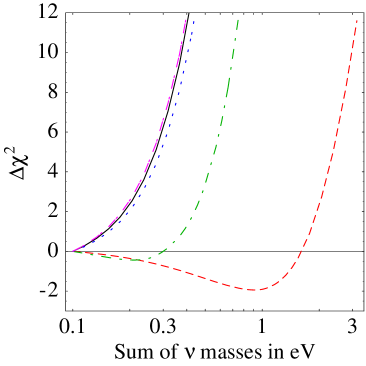
Figure 4: Fit as function of the energy density in freely-streaming slow particles, parameterized by the sum of active neutrino masses, assumed to have the standard abundance $N_{\nu}=3.04$. We studied different combinations of data-sets, as indicated by the legend.

4 Results

In all cases we will report the difference $\Delta\chi^{2}$ with respect to the standard $\Lambda$CDM model (which is individuated by the best fit points in eq. (3) and assumes the existence of only 3 ordinary, massless neutrinos), because this is the significant statistical indicator. Roughly speaking, $\Delta\chi^{2}+\Delta N_{p}=\pm n^{2}$ corresponds to $n$ standard deviations of evidence against or for, where $\Delta N_{p}=N_{p}-N_{p}^{\rm stnd}$ is the number of extra relevant free parameters with respect to $\Lambda$CDM. For the models that we will consider, the not univocally defined $\Delta N_{p}\sim 1$ or 2 is small enough that it does not play a significant rôle. In practice, this means e.g. that $3\sigma$ ranges can be read from fig. 4 or fig. 5 by looking where our curves reach $\Delta\chi^{2}=9$.

We here do not judge the compatibility of a model with data by performing the Pearson $\chi^{2}$ test. According to this test, a model is excluded if the total $\chi^{2}$ is not compatible with its expected value $N\pm\sqrt{2N}$ where $N$ is the number of data points minus the number of free parameters (for $N\gg 1$ the $\chi^{2}$ follows a Gaussian distribution with this mean and variance; for small $N$ the $\chi^{2}$ has a different ‘$\chi^{2}$’ probability distribution). The $\sqrt{2N}$ means that the Pearson $\chi^{2}$ test becomes inefficient when $N\gg 1$, which is the case in cosmological fits, where $N\sim(100\div 1000)$. In practice, this means that a model disfavored at $5\sigma$ by the $\Delta\chi^{2}$ test typically is disfavored only at $1\sigma$ by the $\chi^{2}$ test. A more detailed discussion of these issues can be found in section 4 of [26] (in the context of fits of solar neutrino data).

4.1 Massive neutrinos

Fig. 4 shows the result of our comparison of cosmological data with massive neutrinos. We here assume that only the three active neutrinos exist, and have the standard abundance and temperature. Cosmology is not yet sensitive enough to discriminate neutrinos with normal from inverted hierarchy, but only to heavy quasi-degenerate neutrinos. Therefore the key parameter probed by cosmology is the sum of neutrino masses $\sum m_{\nu}=m_{1}+m_{2}+m_{3}$. Oscillation data imply $\sum m_{\nu}\approx 0.05\,{\rm eV}$ ($0.10\,{\rm eV}$) [1] if neutrinos have strictly normal (inverted) mass hierarchy, and larger values of $\sum m_{\nu}$ are obtained for quasi-degenerate neutrinos. We assumed normal hierarchy at $\sum m_{\nu}=0.05\,{\rm eV}$, inverted hierarchy at $\sum m_{\nu}=0.1\,{\rm eV}$, and degenerate neutrinos at larger $\sum m_{\nu}$.

Within standard cosmology, WMAP3 data alone imply a constraint not plagued by potential systematical problems: we find $\sum m_{\nu}<2.2\,{\rm eV}$ at $95\%$ C.L. (see fig. 4) in agreement with [7, 27]. Adding LSS data (that are more strongly affected by neutrino masses than CMB data) gives stronger constraints, but they are subject to the potential systematic problems discussed in section 3.2. We therefore plotted different lines, that correspond to different combinations of data-sets, with each kind of observable excluded in turn. Our global fit gives

$$\sum m_{\nu}<0.40\,{\rm eV}\qquad\hbox{at 99.9\% C.L.}$$ (8)

in good agreement with [28] and in reasonably good agreement with [18]. We see that SN data have essentially no effect, while Lyman-$\alpha$ data play an important rôle: the constraint becomes about 2 times weaker if Lyman-$\alpha$ data are dropped: $\sum m_{\nu}<0.73\ (0.52)\,{\rm eV}$ at 99.9% (95%) C.L., in good agreement with [28] and in reasonably good agreement with [7].

However, the constraint from the global fit is somewhat stronger than the sensitivity of the data. Indeed, focussing on Lyman-$\alpha$ data, the main effect of neutrino masses at fixed values of other cosmological parameters, consists in reducing the adimensional $\Delta^{2}$, measured by SDSS Lyman-$\alpha$ data with $\pm 0.07$ uncertainty, by about $0.13\sum m_{\nu}/\,{\rm eV}$. However, for massless neutrinos, the global fit already suggests a value of $\Delta^{2}$ about 2 standard deviations below the experimental value, and making neutrinos massive reduces further the expected $\Delta^{2}$. In eq. (8) we avoided reporting a strong but doubtful constraint by choosing a confidence level higher enough than 2 standard deviations.

4.2 Extra freely-streaming massless particles

As usual the ‘number of neutrinos’ $N_{\nu}$ parameterizes the amount of energy in all relativistic freely-streaming degrees of freedom, converted in terms of ‘neutrino equivalents’: $N_{\nu}$ includes the ordinary neutrinos and any extra fermion or boson, as it is formally defined by the relation $\rho_{\rm relativistic}=\rho_{\gamma}\left[1+7/8\ N_{\nu}(T_{\nu}/T)^{4}\right]$, where $T_{\nu}/T=(4/11)^{1/3}$ at $T\ll m_{e}$. Standard cosmology with 3 neutrinos predicts $N_{\nu}\approx 3.04$ (the deviation from 3 being due to the incomplete $\nu_{e}$ decoupling at the time of the beginning of $e^{+}e^{-}$ annihilations, plus other small corrections). Our global fit gives

$$N_{\nu}=5\pm 1$$ (9)

and the continuous line in fig. 5a shows the precise form of the $\Delta\chi^{2}$. We checked that using the first release of WMAP data our result agrees with the various analyses published in the literature [30].

In general, results of global fits can be mislead by problems in any of the pieces of data they contain; in this case the validity of the global fit appears particularly doubtful: $N_{\nu}$ is dominantly determined by non-CMB data, and giving slightly different weight to them can significantly affect the fit because different pieces of data prefer different values of $N_{\nu}$. In particular, the $2\sigma$ preference for $N_{\nu}>3$ is mainly due to the $2\sigma$ anomaly in the Lyman-$\alpha$ measurement of the power spectrum: fig. 5a shows that omitting Lyman-$\alpha$ one recovers excellent agreement with the standard value $N_{\nu}=3$. The agreement with and between the up-to-date analyses performed by the WMAP Team [7] and by [18] is imperfect; in particular the revised version of [18] claims a $3\sigma$ preference for $N_{\nu}>3$.

            

Figure 5: Fig. 5a): fit as function of the energy density in freely-streaming relativistic particles, parametrized by the usual ‘number of neutrinos’ $N_{\nu}$. Fig. 5b): fit as function of the energy density in extra interacting relativistic particles, with abundance parametrized by $\Delta N_{\nu}$. We studied different combinations of data-sets, as indicated by the legend.

4.3 Extra massless particles interacting among themselves

In the previous section we considered extra (massless) particles with negligible interactions, that therefore freely move on cosmological scales. We now consider the opposite limit: extra (massless) particles that interact among themselves with a mean free path smaller than relevant cosmological scales, such that inhomogeneities in their energy density evolve in a different way. Concrete examples are an elementary scalar with a quartic self-interaction or any particle with low compositeness scale, obtained e.g. if some extra QCD-like gauge group becomes strongly coupled at an energy much lower than the QCD scale. In the tight coupling limit this system is described by a fluid: its density and velocity perturbations $\delta$ and $v$ obey the standard fluid equations (in the conformal Newtonian gauge and in linear approximation):

$$\dot{\delta}=-4\dot{\Phi}-\frac{4}{3}kv,\qquad\dot{v}=k\Psi+\frac{k\delta}{4}$$ (10)

where a dot denotes derivative with respect to conformal time, $k$ is the wavenumber, $\Phi$ and $\Psi$ are the scalar perturbations in the metric (in the notations of [31]).

Fig. 5b shows the constraint on the density of the extra particles, that we parameterize in terms of the usual ‘equivalent number of neutrinos’ $\Delta N_{\nu}\geq 0$: the global fit gives

$$\Delta N_{\nu}=0\pm 1.3.$$ (11)

Data do not favor the presence of extra massless particles interacting among themselves. Dropping Lyman-$\alpha$ data makes the $1\sigma$ constraint two times more stringent. Fig. 5b shows that the interval allowed at $n$-$\sigma$ is not $n$ times larger than the $1\sigma$ interval.

      

Figure 6: Fig. 6a: how the global fit constrains the presence of extra freely-streaming particles with abundance $\Delta N_{\nu}$ and mass $m_{\rm s}$. Shaded regions are allowed. Fig. 6b: the analogous result for extra interacting particles.

4.4 Extra freely-streaming massive particles

We here assume that the ordinary neutrinos have cosmologically negligible masses (e.g. $0.05\,{\rm eV}$ [1]), and add extra freely-streaming particles, with abundance $\Delta N_{\nu}$, mass $m_{\rm s}$ and the same temperature as the ordinary neutrinos. We have chosen the notation $\Delta N_{\nu}$ and $m_{\rm s}$ because, although the constraints we obtain here apply to a generic freely-streaming fluid (but not to extra interacting particles, studied in the next sections), sterile neutrinos of mass $m_{\rm s}$ are by far the most popular specific realization. Sterile neutrino models allow one to compute the abundance $\Delta N_{\nu}$ in terms of oscillation parameters (non-minimal scenarios introduce extra parameters, such as particle/anti-particle asymmetries), and $\Delta N_{\nu}$ can acquire a small, sub-thermal value, that stays constant after neutrino decoupling at $T\sim{\rm MeV}$. We here assume that $\Delta N_{\nu}$ keeps an arbitrary constant value at the much lower temperatures relevant for CMB and LSS observables. The present energy density is

$$\Omega_{\rm s}\equiv\frac{\rho_{\rm s}}{\rho_{\rm cr}}=\frac{0.01}{h^{2}}\frac{m_{\rm s}\cdot\Delta N_{\nu}}{\,{\rm eV}}.$$ (12)

This case is characterized by 2 new parameters: therefore we must make 2-dimensional plots, so we prefer not to show how the fit changes by considering various different data-sets. Fig. 6a shows the global fit. We can distinguish three regions. For small $m_{\rm s}$ and large $\Delta N_{\nu}\,\raise 1.29167pt\hbox{$>$\kern-7.5pt\lower 4.30554pt\hbox{$\sim$}}\,1$, data disfavor a too large number of relativistic particles around recombination. In the intermediate region the extra particles behave as warm Dark Matter: their abundance is constrained to be $\Omega_{\rm s}\,\raise 1.29167pt\hbox{$<$\kern-7.5pt\lower 4.30554pt\hbox{$\sim$}}\,0.01$ dominantly by Lyman-$\alpha$ and LSS data. For larger $m_{\rm s}\gg\,{\rm keV}$ the extra particle behave as cold enough Dark Matter and sterile densities as large as $\Omega_{\rm s}\approx 0.22$ are allowed. Assuming one thermalized freely-streaming sterile neutrino ($\Delta N_{\nu}=1$) we find that its mass is constrained to be $m_{\rm s}<0.7\,{\rm eV}$ at $99.9\%$ C.L., a range incompatible with the mass suggested by the LSND anomaly [33, 1]. Our results have some overlap and substantial agreement with [6, 34, 18, 35].

4.5 Extra massive particles interacting among themselves

We now assume that the extra particles discussed in section 4.3 have a non negligible mass $m_{\rm s}$ and are stable, such that when the temperature $T$ falls below $m_{\rm s}$ they form a non-relativistic relic. (Alternatively, they could decay into freely-streaming particles realizing a more complicated situation that is intermediate between the one studied in the previous section and in this section). Particles with this behavior are exemplified in section 4.3. In the tight coupling limit this system is described by a fluid, and the massless fluid equations in eq. (10) generalize to

$$\dot{\delta}=-(1+w)(3\dot{\Phi}+kv)-3\frac{\dot{a}}{a}(c_{\rm s}^{2}-w)\delta,\qquad\dot{v}=k\Psi-\frac{\dot{a}}{a}(1-3c_{\rm s}^{2})v+\frac{c_{\rm s}^{2}}{1+w}k\delta$$ (13)

where $w\equiv p/\rho$ and $c_{\rm s}^{2}\equiv\delta p/\delta\rho$ is the squared sound speed. We fix the equation of state of the fluid by assuming that its average energy density $\rho$ and pressure $p$ is the one of $2\cdot\Delta N_{\nu}$ dof decoupled from the rest of the thermal plasma:

$$\rho=2\cdot\Delta N_{\nu}\int\frac{d^{3}p}{(2\pi)^{3}}E~{}e^{-p/T_{\rm s}},\qquad p=2\cdot\Delta N_{\nu}\int\frac{d^{3}p}{(2\pi)^{3}}\frac{p^{2}}{3E}~{}e^{-p/T_{\rm s}},\qquad E=\sqrt{p^{2}+m_{\rm s}^{2}}.$$ (14)

In practice this just means that the fluid interpolates between relativistic and non relativistic matter: $w\simeq c_{\rm s}^{2}\simeq 1/3$ at $T\gg m_{\rm s}$ and $w\simeq c_{\rm s}^{2}\simeq 0$ at $T\ll m_{\rm s}$. A more sophisticated treatment seems unnecessary. For simplicity we have adopted Boltzmann statistics in eq. (14). Again, the parameter $\Delta N_{\nu}$ tells the initial abundance of the extra particles in the usual ‘neutrino-equivalent’ units. We again assume that $T_{\rm s}=T_{\nu}$, such that this extra component is described by two parameters: its abundance $\Delta N_{\nu}$ and its mass $m_{\rm s}$.

Fig. 6b shows the result of the global fit: interacting extra particles are constrained in a slightly stronger way than freely-streaming extra particles (at not too low C.L.). Notice that, like in the case of massive freely-streaming sterile neutrinos, cosmology disfavors the mass values suggested by the LSND anomaly [33, 1] also in this opposite limit of tightly-interacting sterile neutrinos, suggesting that intermediate cases might also be not viable.

A. de Gouvea suggested us one possible new economical interpretation of the LSND anomaly, in terms of decays among active-only neutrinos. This would need some order one couplings with a light scalar, making neutrinos cosmologically interacting: as we have seen a global fit of cosmological data disfavors this possibility. Furthermore, a preliminary analysis indicates that the needed decay is incompatible with SuperKamiokande atmospheric neutrino data at about $3\sigma$ C.L.

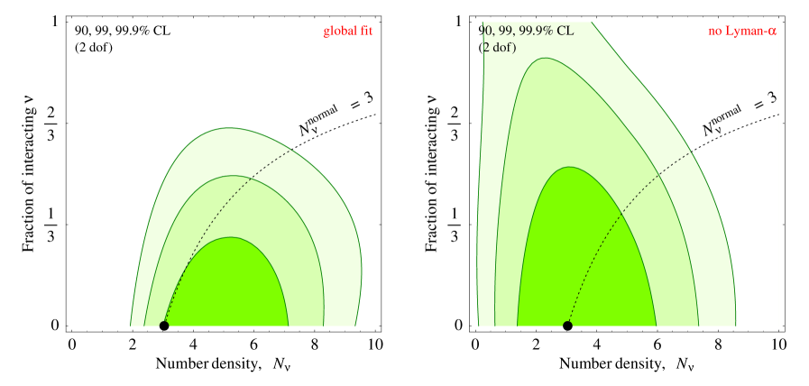
Figure 7: Global fit of the total relativistic energy density (parametrized by the usual ‘number of neutrinos’ $N_{\nu}$), and of its interacting fraction. The dot shows the SM prediction, and along the dotted line the number of normal freely-streaming neutrinos keeps its standard value.

4.6 Massless neutrinos interacting with a massless boson

So far we added extra light particles, free or interacting among themselves. We now assume that ordinary neutrinos are involved in interactions with these extra particles. More specifically, we consider $N_{\nu}^{\rm normal}$ neutrinos that behave normally, while $N_{\nu}^{\rm int}$ neutrinos are involved in the interactions with extra scalars $\phi$, such that these interacting $N_{\nu}^{\rm int}$ neutrinos no longer free stream, but form a tightly coupled fluid together with the scalars.

Following [36, 37] we assume that the energy and pressure density of this fluid are given in the homogenous limit by

$$\rho=2N_{\nu}^{\rm int}\rho_{F}^{\rm eq}(m_{\nu},T_{\rm fl})+N_{\phi}\rho_{B}^{\rm eq}(m_{\phi},T_{\rm fl}),\qquad p=2N_{\nu}^{\rm int}p_{F}^{\rm eq}(m_{\nu},T_{\rm fl})+N_{\phi}p_{B}^{\rm eq}(m_{\phi},T_{\rm fl})$$ (15)

where $\rho_{F}^{\rm eq}(m,T)$ and $p_{F}^{\rm eq}(m,T)$ are the energy and pressure density of one fermionic degree of freedom with mass $m$ in thermal equilibrium at temperature $T$, and $\rho_{B}^{\rm eq}$ and $p_{B}^{\rm eq}$ are the analogous quantities for one bosonic degree of freedom. The temperature $T_{\rm fl}$ of the fluid is computed by assuming that it equals the ordinary neutrino temperature at $T\gg m_{\nu},m_{\phi}$, and that the fluid cools down adiabatically. This fixes the fluid equation of state $w$ and its sound speed $c_{\rm s}$, and inhomogeneities evolve as dictated by eq. (13). Summarizing, this system is described by the following parameters: $N_{\nu}^{\rm normal}$, $N_{\nu}^{\rm int}$, $N_{\phi}$, $m_{\nu}$, $m_{\phi}$.

In this section we assume that $m_{\nu}$ and $m_{\phi}$ are negligibly small, such that $w=c_{\rm s}^{2}=1/3$ (relativistic fluid). Then, the ratio $N_{\nu}^{\rm int}/N_{\phi}$ becomes essentially irrelevant, such that the system can be described by just two parameters: i) the total energy density in relativistic particles, that we describe by the usual ‘number of neutrinos’ $N_{\nu}=N_{\nu}^{\rm normal}+N_{\nu}^{\rm int}+4N_{\phi}/7$, that remains constant; ii) the energy fraction $R=N_{\nu}^{\rm int}/N_{\nu}$ that contributes to the fluid. The remaining fraction $1-R=N_{\nu}^{\rm normal}/N_{\nu}$ freely streams. In standard cosmology $R=0$ and $N_{\nu}=N_{\nu}^{\rm normal}=3.04$. Fig. 7 shows how a global fit of present data determines these two parameters. The ‘all interacting’ case ($R=1$) is disfavored at $4\sigma$ at least (i.e. $\min\chi^{2}(N_{\nu},R=1)-\chi^{2}(N_{\nu}=3,R=0)\,\raise 1.29167pt\hbox{$>$\kern-7.5pt\lower 4.30554pt\hbox{$\sim$}}\,16$) and at $3\sigma$ if Lyman-$\alpha$ data are dropped. As in the case of massive neutrinos, Lyman-$\alpha$ data make the constraint slightly stronger than the sensitivity. Two previous analyses claimed different results: our constraints are somewhat stronger than in [37] (possibly because we use the most recent data set) and weaker than in [36].

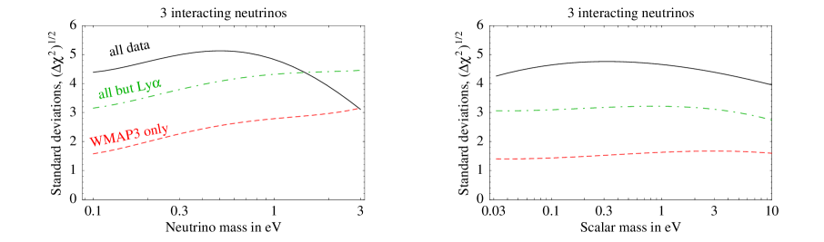
Figure 8: Number of standard deviations, defined as $(\chi^{2}-\chi^{2}_{0})^{1/2}$ (where $\chi^{2}_{0}$ is the best $\Lambda\rm CDM$ fit with massless neutrinos) at which cosmological data disfavor a fluid of 3 neutrinos interacting with a scalar assuming massive neutrinos and massless scalar (fig. 8a) or massless neutrinos and massive scalar (fig. 8b). The different lines correspond to different data-sets: global fit (continuous black line), Lyman-$\alpha$ data dropped (dot-dashed green line), WMAP3 only (dashed red line).

4.7 Massive neutrinos interacting with a massless boson

We now explore how the situation changes if neutrinos have a non vanishing mass $m_{\nu}$. We focus on the most interesting limiting case: $R=0$ i.e. we now assume that all neutrinos are involved in the interaction. This is interesting because it means that the cosmological bound on neutrino masses no longer applies, because when $T\,\raise 1.29167pt\hbox{$<$\kern-7.5pt\lower 4.30554pt\hbox{$\sim$}}\,m_{\nu}$ all neutrinos annihilate or decay into massless $\phi$ particles. Scenarios of this kind have been proposed for a number of reasons [38, 39, 40]. We again assume that neutrinos initially have the standard abundance, and that bosons initially have the minimal abundance, $N_{\phi}=1$ (one real scalar). After that all neutrinos annihilate into $\phi$, they acquire a relativistic energy density corresponding to an equivalent number of neutrinos $N_{\nu}(T\,\raise 1.29167pt\hbox{$<$\kern-7.5pt\lower 4.30554pt\hbox{$\sim$}}\,m_{\nu})=4/7(25/4)^{4/3}\sim 6.6$.

Fig. 8a shows how much this non-standard cosmology is disfavored as a function of $m_{\nu}$ (standard cosmology is not recovered for any value of $m_{\nu}$). For $m_{\nu}\ll\,{\rm eV}$ the result is similar to the case $m_{\nu}=0$, already discussed in section 4.6: this scenario is disfavored at about $4\sigma$ by the global fit. As already noticed in [37], the scenario becomes less disfavored for $m_{\nu}\,\raise 1.29167pt\hbox{$>$\kern-7.5pt\lower 4.30554pt\hbox{$\sim$}}\,\,{\rm eV}$ (beta decay data demand $m_{\nu}\,\raise 1.29167pt\hbox{$<$\kern-7.5pt\lower 4.30554pt\hbox{$\sim$}}\,2\,{\rm eV}$ [1]). We find that WMAP3 data (dashed lines in fig.s 8) are more constraining than the WMAP1 data analyzed in [37].

We do not consider intermediate scenarios where only one or two massive neutrinos interact with the scalar: both the constraint on neutrino masses and on their free-streaming applies, but in a milder form [37].

4.8 Massless neutrinos interacting with a massive boson

We conclude studying the opposite limit: neutrinos have a negligibly small mass, while the scalar has a mass $m_{\phi}$. The considerations of the previous section still apply, with the rôle of neutrinos and interacting particles interchanged: since neutrinos have more degrees of freedom than one scalar, the radiation density increases in a mild way when $T$ drops below $m_{\phi}$. Fig. 8b shows how much this non-standard cosmology is disfavored as a function of $m_{\phi}$: we find almost no dependence on $m_{\phi}$: this scenario is disfavored at about $4\sigma$. For large enough $m_{\phi}$, depending on the model, interactions mediated by $\phi$ must become weak enough that neutrinos recover their standard freely-streaming behavior.

5 Conclusions

We compared a non exhaustive but representative casistics of how cosmology is affected by extra light particles (with sub-keV masses), or by standard and non-standard properties of neutrinos, using CMB, LSS, Lyman-$\alpha$, BAO, SN data.

• First, we considered ordinary massive neutrinos. We obtain the cosmological bound on neutrino masses, $\sum m_{\nu}\,\raise 1.29167pt\hbox{$<$\kern-7.5pt\lower 4.30554pt\hbox{$\sim$}}\,0.40\,{\rm eV}$ at $99.9\%$ C.L. and fig. 4a shows that the relatively less safe observations play a crucial rôle.

• The density of initially relativistic particles can be parameterized in terms of the usual number $N_{\nu}$ of equivalent neutrinos. Assuming that all the $N_{\nu}$ relativistic particles freely stream, we find that their density is constrained to be $N_{\nu}=5\pm 1$. The $2\sigma$ preference for $N_{\nu}>3$ is mainly due to the $2\sigma$ anomaly in the Lyman-$\alpha$ measurement of the matter power spectrum.

• Assuming ordinary neutrinos plus an extra component of interacting particles, we find $\Delta N_{\nu}=0\pm 1.3$. Fig. 7 shows how data constrain the intermediate case where both kinds of relativistic particles are present. It is interesting that the uncertainty on $\Delta N_{\nu}$ is decreasing below 1.

• The extra light particles might have a mass $m$ and an abundance $\Delta N_{\nu}$. Fig. 6 shows how data constrain these parameters in the two limiting cases that these extra particles freely stream (fig. 6a) or interact among themselves (fig. 6b).

• Finally, we considered one extra scalar of mass $m_{\phi}$ that interacts with neutrinos of mass $m_{\nu}$. We find that this scenario is strongly disfavored by the global fit, at about $4\sigma$.

All these results are based on assumptions and subject to caveats, that we discussed in the text. Technically, our analysis somewhat differs from typical analyses because we used a code developed by us and dealt with statistics using Gaussian analytical techniques, that become adequate nowadays that observations are rich and precise enough. Eq.s  (3) and (5) allow to check how well we reproduce the standard results for standard cosmology.

Acknowledgments

We thank Ben Allanach, Paolo Creminelli, Concha Gonzalez-Garcia, Danilo Marchesini, Riccardo Rattazzi, Adam Riess and Licia Verde for discussions and clarifications and John Kovac, Hiranya Peiris and Jonathan Sievers for communications. The authors thank the Galileo Galilei Institute for Theoretical Physics in Firenze for the hospitality and INFN for partial support during the completion of this work. The work of M.C. is supported in part by the USA DOE-HEP Grant DE-FG02-92ER-40704. M.C. thanks the Service de Physique Théorique of CEA-Saclay for the hospitality during the completion of this work.

References

- [1] For a review and references see A. Strumia and F. Vissani, hep-ph/0606054.
- [2] J. Lesgourgues and S. Pastor, astro-ph/0603494.
- [3] S. Bashinsky and U. Seljak, Phys. Rev. D69 (2004) 083002 [astro-ph/0310198].
- [4] See S. Kachru, R. Kallosh, A. Linde, S. Trivedi, Phys. Rev. D68 (2003) 046005 [hep-th/0301240] for complicated string models.
- [5] LEP and SLD collaborations, Phys. Rept. 427 (2006) 257 [hep-ex/0509008].
- [6] M. Cirelli, G. Marandella, A. Strumia and F. Vissani, Nucl. Phys. B708 (2005) 215 [hep-ph/0403158].
- [7] D.N. Spergel et al. (WMAP Science Team), astro-ph/0603449.
- [8] CMBfast: U. Seljak, M. Zaldarriaga, Astrophys. J. 469 (1996) 437. Formulæ for and are given in Z. Zaldarriaga, U. Seljak, Phys. Rev. D55 (1997) 1830. CAMB, a more efficient implementation by A. Lewis and A. Challinor, camb.info.
- [9] U. Seljak, Astrophys. J. 435 (1994) L87 [astro-ph/9406050].
- [10] C.P. Ma and E. Bertschinger, Astrophys. J. 455 (1995) 7 [astro-ph/9506072].
- [11] S. Seager, D. Sasselov, D. Scott, Astrophys. J. Suppl. 128 (2000) 407 [astro-ph/9912182]. Web page: www.astro.ubc.ca/people/scott/recfast.html.
-
[12]
See e.g.
wolfram.com/products/mathematica/index.html or en.wikipedia.org/wiki/Mathematica. - [13] G. Hinshaw et al. (WMAP Science Team), astro-ph/0603451. L. Page et al., astro-ph/0603450.
- [14] See M. Limon et al. on lambda.gsfc.nasa.gov/product/map.
- [15] Data from other CMB experiments, for the TT spectrum: C.L. Kuo et al. (ACBAR collaboration), Astrophys. J. 600 (2004) 32 [astro-ph/0212289], web page cosmology.berkeley.edu/group/swlh/acbar. A.C.S. Readhead et al. (CBI collaboration), Astrophys. J. 609 (2004) 498 [astro-ph/0402359], web page www.astro.caltech.edu/~tjp/CBI. W.C. Jones et al. (Boomerang collaboration), astro-ph/0507494, web page cmb.phys.cwru.edu/boomerang. K. Grainge et al. (VSA collaboration), Mon. Not. Roy. Astron. Soc. 341 (2003) L23 [astro-ph/0212495], web page www.mrao.cam.ac.uk/telescopes/vsa. For the TE spectrum: F. Piacentini et al. (Boomerang collaboration), astro-ph/0507507. E.M. Leitch, J.M. Kovac, N.W. Halverson, J.E. Carlstrom, C. Pryke and M.W.E. Smith (DASI collaboration), astro-ph/0409357. For the EE spectrum: J.L. Sievers et al. (CBI collaboration), astro-ph/0509203, supplemented with the details in A.C.S. Readhead et al., Science 306 (2004) 836 [astro-ph/0409569]. T.E. Montroy et al. (Boomerang collaboration), astro-ph/0507514. DASI collaboration as cited above, astro-ph/0409357. D. Barkats et al. (CAPMAP collaboration), Astrophys. J. 619 (2005) L127 [astro-ph/0409380].
- [16] SDSS collaboration, Astrophys. J. 606 (2004) 702 [astro-ph/0310725], web page www.sdss.org, data available at the web page space.mit.edu/home/tegmark/sdss.html. The more recent data in N. Padmanabhan et al., astro-ph/0605302 are not publicly available.
- [17] 2dFGRS collaboration, Mon. Not. Roy. Astron. Soc. 362 (2005) 505 [astro-ph/0501174], web page www.mso.anu.edu.au/2dFGRS.
- [18] U. Seljak, A. Slosar, P. McDonald, astro-ph/0604335, version 3.
- [19] D.J. Eisenstein et al., Astrophys. J. 633 (2005) 560 [astro-ph/0501171].
- [20] R.A.C. Croft et al., Astrophys. J. 581 (2002) 20 [astro-ph/0012324].
- [21] SDSS collaboration, Astrophys. J. 635 (2005) 761 [astro-ph/0407377]. See also: SDSS collaboration, Astrophys. J. Suppl. 163 (2006) 80 [astro-ph/0405013].
- [22] M. Viel, M.G. Haehnelt and V. Springel, Mon. Not. Roy. Astron. Soc. 354 (2004) 684 [astro-ph/0404600]. M. Viel and M.G. Haehnelt, Mon. Not. Roy. Astron. Soc. 365 (2006) 231 [astro-ph/0508177]. M. Viel, M.G. Haehnelt and A. Lewis, astro-ph/0604310.
- [23] A.G. Riess et al. (Supernova Search Team - GOODS/HST compilation), Astrophys. J. 607 (2004) 665 [astro-ph/0402512].
- [24] P. Astier et al. (Supernova Legacy Survey collaboration), Astron. Astrophys. 447 (2006) 31 [astro-ph/0510447].
- [25] The HST key project measurement of the Hubble constant: W.L. Freedman et al., Astrophys. J. 553 (2001) 47 [astro-ph/0012376].
- [26] P. Creminelli, G. Signorelli and A. Strumia, JHEP 0105 (052) 2001 [hep-ph/0102234].
- [27] M. Fukugita, K. Ichikawa, M. Kawasaki, O. Lahav, astro-ph/0605362.
- [28] A. Goobar, S. Hannestad, E. Mortsell and H. Tu, astro-ph/0602155.
- [29] R. Bowen, S. Hansen, A. Melchiorri, J. Silk, R. Trotta, Mon. Not. Roy. Astron. Soc. 334 (2002) 760 [astro-ph/0110636].
- [30] E. Pierpaoli, Mon. Not. Roy. Astron. Soc. 342 (2003) L63 [astro-ph/0302465]. P. Crotty, J. Lesgourgues and S. Pastor, Phys. Rev. D67 (2003) 123005 [astro-ph/0302337]. S. Hannestad, JCAP 0601 (2006) 001 [astro-ph/0510582].
- [31] S. Dodelson, “Modern cosmology”, Academic Press, 2003.
- [32] U. Seljak, A. Makarov, P. McDonald, H. Trac, astro-ph/0602430. M. Viel, J. Lesgourgues, M. Haehnelt, S. Matarrese, A. Riotto, Phys. Rev. Lett. 97 (2006) 071301 [astro-ph/0605706].
- [33] LSND collaboration, Phys. Rev. D64 (2001) 112007 [hep-ex/0104049].
- [34] S. Dodelson, A. Melchiorri and A. Slosar, astro-ph/0511500.
- [35] S. Hannestad and G. Raffelt, JCAP 0404 (2004) 008 [hep-ph/0312154]. P. Crotty, J. Lesgourgues and S. Pastor, Phys. Rev. D69 (2004) 123007 [hep-ph/0402049]. S. Hannestad and G. G. Raffelt, astro-ph/0607101.
- [36] S. Hannestad, JCAP 0502 (2005) 011 [astro-ph/0411475]. S. Hannestad, G. Raffelt, Phys. Rev. D72 (2005) 103514 [hep-ph/0509278].
- [37] N. Bell, E. Pierpaoli, K. Sigurdson, Phys. Rev. D73 (2006) 063523 [astro-ph/0511410].
- [38] J. F. Beacom, N. F. Bell and S. Dodelson, Phys. Rev. Lett. 93 (2004) 121302 [astro-ph/0404585].
- [39] Z. Chacko, L. Hall, T. Okui, S. Oliver, Phys. Rev. D70 (2004) 085008 [hep-ph/0312267]. Z. Chacko, L. J. Hall, S. J. Oliver and M. Perelstein, Phys. Rev. Lett. 94 (2005) 111801 [hep-ph/0405067]. R. N. Mohapatra and S. Nasri, Phys. Rev. D71 (2005) 053001 [hep-ph/0407194].
- [40] P. Hung, hep-ph/0010126. P. Gu, X. Wang, X. Zhang, Phys. Rev. D68 (2003) 087301 [hep-ph/0307148]. R. Fardon, A. E. Nelson, N. Weiner, JCAP 0410 (2004) 005 [astro-ph/0309800].