The VIMOS-VLT Deep Survey

Abstract

Aims. In this paper we discuss the mix of star-forming and passive galaxies up to z$\sim$2, based on the first epoch VIMOS-VLT Deep Survey (VVDS) data.

Methods. We compute rest-frame magnitudes and colors and analyse the color-magnitude relation and the color distributions. We also use the multi-band VVDS photometric data and spectral templates fitting to derive multi-color galaxy types. Using our spectroscopic dataset we separate galaxies based on a star-formation activity indicator derived combining the equivalent width of the [OII] emission line and the strength of the D_n(4000) continuum break.

Results. In agreement with previous works we find that the global galaxy rest-frame color distribution follows a bimodal distribution at z$\leq$1, and we establish that this bimodality holds up to at least z=1.5. The details of the rest-frame color distribution depend however on redshift and on galaxy luminosity, with faint galaxies being bluer than the luminous ones over the whole redshift range covered by our data, and with galaxies becoming bluer as redshift increases. This latter blueing trend does not depend, to a first approximation, on galaxy luminosity. The comparison between the spectral classification and the rest-frame colors shows that about 35-40 % of the red objects are in fact star forming galaxies. Hence we conclude that the red sequence cannot be used to effectively isolate a sample of purely passively evolving objects within a cosmological survey. We show how multi-color galaxy types have a slightly higher efficiency than rest-frame color in isolating the passive, non star-forming galaxies within the VVDS sample. Connected to these results is also the finding that the color-magnitude relations derived for the color and for the spectroscopically selected early-type galaxies have remarkably similar properties, with the contaminating star-forming galaxies within the red sequence objects introducing no significant offset in the rest frame colors. Therefore the average color of the red objects does not appear to be a very sensitive indicator for measuring the evolution of the early-type galaxy population.

1 Introduction

Early-type galaxies are the preferred target for studies on how and when galaxies were formed, because of the simpler task of modeling an old stellar population undergoing passive evolution compared to modeling a young population continuously modified by an irregular star formation history. Over the last few years, mostly in response to the accumulating evidence in favor of a predominantly old stellar population within early type galaxies (see for a complete review Renzini 2006), the discussion has focused onto two main areas: the history of stellar formation and how and when stars assembled into galaxies. Still, a fundamental pre-requisite for such studies is to isolate from cosmological surveys a sample of early-type galaxies representative of the true galaxy population at all epochs probed.

Commonly used galaxy classification schemes are based purely on the morphological appearance of galaxies. It is well known however that galaxies follow a number of scaling relations involving their stellar populations and their morphological, structural and photometric parameters. Compared to their late-type counterparts, early-type galaxies have been found to be redder (color-morphological type relation, Roberts & Haynes 1994), more luminous (color-magnitude relation, Visvanathan & Sandage 1977; Tully et al. 1982), to be located in denser environments (morphology-density relation, Dressler 1980), and to have a star formation history that takes place over shorter time-scales (Sandage 1986; Gavazzi et al. 2002).

Cosmological survey studies, faced with the difficulty of obtaining a morphological classification for all the galaxies in their sample, have often tried to take advantage of those relations to define an alternate classification scheme. Galaxy color, which is by far the easiest parameter to measure for a full survey sample, has been most commonly used as a substitute for morphological information. Lately this practice has become even more commonplace, since the galaxy rest-frame color distributions have been found to be clearly bimodal. This bimodality was well known to exist within clusters of galaxies, where the early- and late-type galaxies follow two rather distinct color-magnitude relations, as discussed by Visvanathan & Sandage (1977) and Bower et al. (1992) for early-type galaxies and Tully et al. (1982) and Gavazzi et al. (1996) for late-type ones. That the same bimodality was present in a general field sample was first noticed in the local universe by Strateva et al. (2001) using the SDSS galaxies sample, and afterwards discussed by many other authors (see, as an example, Baldry et al. 2004a, b). Bell et al. (2004b) (hereafter B04) and Weiner et al. (2005) detected the rest-frame color bimodality also at higher redshifts up to z$\sim$1, respectively in the COMBO-17 and DEEP2 data.

Color bimodality is interpreted as just one specific signature introduced by the general processes controlling galaxy formation and evolution (Menci et al. 2005; Dekel & Birnboim 2006). Other similar signatures are observed, since bimodality has been found to be a characteristic in the distribution of many other observables like H_α emission (Balogh et al. 2004), 4000 $\AA$ break (Kauffmann et al. 2003b), star formation history (Brinchmann et al. 2004), or clustering (Budavári et al. 2003; Meneux et al. 2006).

Because of the age of their stellar population, early-type galaxies are expected to have very red optical colors over a rather large redshift range. This expectation has been confirmed in clusters of galaxies, where the red-sequence for morphologically selected early-type galaxies has been observed up to z$\sim$1.2 (Kodama & Arimoto 1997; Stanford et al. 1998). As a result the red color has often been used as a tracer to isolate samples of early-type galaxies. Most recently the widespread acceptance of color bimodality has resulted in the use of red-sequence galaxies (those that populate the red peak of the color bimodal distribution) to study the evolution of early-type galaxies, implicitly assuming this red population to be entirely composed of old, passively evolving objects.

However, while most of the early-type galaxies are indeed red, they are possibly not the only red objects included in a survey sample. Attempts at quantifying the contamination of non early-type, passive objects within samples of red galaxies include both studies focused on Extremely Red Objects (EROs), and more general surveys which target the whole bulk of the galaxy population. Among EROs, Cimatti et al. (2002), using spectroscopic data for 45 objects, find a roughly equal proportion of early-type, passive galaxies and of dusty starburst objects. Among less extreme objects, in the local Universe Strateva et al. (2001) reported a significant fraction (20%) of galaxies morphologically later than Sa in the red galaxy population. This result is confirmed using the data for galaxies in the Virgo Cluster and in the Coma Supercluster provided by the GOLDMine database (Gavazzi et al. 2003). At intermediate redshift (up to $z\sim 1$) various studies are confirming these results (see for example Kodama et al. 1999; Bell et al. 2004a), while the nature of red galaxies at higher redshift is less clear. However, there are indications that the fraction of morphologically late-type galaxies with red colors could be even higher at $z\gtrsim\leavevmode\nobreak\ 1$ (Strateva et al. 2001), in agreement with the findings based on EROs studies.

In this work we use VIMOS-VLT Deep Survey photometric and spectroscopic data (VVDS, see Le Fèvre et al. 2005) to compare the galaxy population that can be isolated by using either a red color selection criterion or a spectro-photometric classification. Although neither of these selection criteria can be considered entirely equivalent to a morphological classification in isolating a sample of early-type galaxies, our comparison does provide an estimate for the uncertainties involved in selecting those objects within a cosmological survey sample.

The paper is organized as follows. In section 2 we describe the VVDS galaxy sample, the data we use in this work and we discuss the effect that the VVDS selection function could have on our work. In section 3 we analyse the rest-frame color distributions and we demonstrate that the color bimodality is present up to at least z=1.5. Then we study the color bimodality as a function of redshift and of galaxy luminosity. In section 4 we focus on the red-sequence galaxies studying their color-magnitude relation. In section 5, we analyse in detail the red-sequence objects showing how this population is contaminated by a non negligible fraction of starforming objects. We use the strong bimodality observed in the EW([OII])-D_n(4000) distribution to isolate a sample of early-type galaxies less contaminated by star-forming galaxies than a simple color-magnitude selection. Finally in section 6 we discuss the color evolution of this sample.

All magnitudes are given in the Johnson-Kron-Cousin system; the adopted cosmology is the standard $\Omega_{m}=0.3$, $\Omega_{\Lambda}=0.7$ and $H_{0}=70\leavevmode\nobreak\ km\leavevmode\nobreak\ s^{-1}\leavevmode\nobreak\ Mpc^{-1}$.

2 Sample description

2.1 The data

2.1.1 Observations

Our sample is selected from the first epoch VVDS-Deep spectroscopic sample within the VVDS-0226-04field (hereafter F02) (see Le Fèvre et al. 2005). This is derived from a purely magnitude limited sample (hereafter “photometric sample”), including all objects in the magnitude range 17.5 $\leq I_{AB}\leq$ 24.0 from a complete, deep photometric survey (Le Fèvre et al. 2004).

The whole 1.2 deg² field has been imaged in $B,V,R$ and $I$ with the wide-field 12K mosaic camera at the Canada-France-Hawaii Telescope (CFHT), reaching the limiting magnitudes of $B_{AB}\sim 26.5,V_{AB}\sim 26.2,R_{AB}\sim 25.9,I_{AB}\sim 25.0$. Data are complete and free from surface brightness selection effects down to $I_{AB}\leq 24.0$ (see for details McCracken et al. 2003). U-band data, taken with the Wide-Field Imager at the ESO/MPE 2.2m telescope, are available for a large fraction of the field, to the limiting magnitude of $U_{AB}\sim 25.4$ (Radovich et al. 2004). In all bands, apparent magnitudes have been measured using Kron-like elliptical apertures (the same in all bands), with a minimum Kron radius of 1.2 arcsec, and corrected for the Galactic extinction using the Schlegel dust maps (Schlegel et al. 1998). The median extinction correction in the $I$ band is $\sim 0.05$ magnitudes.

Spectroscopic observations for about 23% of the objects included in the photometric magnitude limited sample have being carried out with the VIsible Multi Object Spectrograph (VIMOS, see LeFevre et al. 2003), on the UT3 unit telescope of the ESO Very Large Telescope. The spectroscopic sample is close to be a perfectly random subset of the parent photometric sample, with only a small bias against large angular-size objects which can be easily corrected for (see Ilbert et al. 2005; Bottini et al. 2005).

Observations have been reduced with the VIMOS Interactive Pipeline and Graphical Interface software package (VIPGI, see Scodeggio et al. 2005; Zanichelli et al. 2005). A redshift measurement has been derived for 9036 galaxies with a success rate which is mildly dependent on both the galaxy apparent magnitude and its redshift (see the discussion on the Spectroscopic Sampling Rate and Figures 2 and 3 in Ilbert et al. 2005). The median redshift for the whole spectroscopic sample is $z=0.76$ (see Figure 25 in Le Fèvre et al. 2005).

The sample we use for this work is composed of all the galaxies with secure identification and redshift measurement (z quality flags 2,3,4,9 in Le Fèvre et al. 2005) in the F02 spectroscopic sample, with the restriction of having $z\leq 2.0$, in order to ensure that the observed optical and near-infrared magnitudes provide a reasonably close bracketing for the rest-frame optical magnitudes we use in our analysis. A total of 6291 galaxies are included in this sample with a measured B, V, R and I magnitude; hereafter we will refer to this sample as “complete sample”.

2.1.2 Rest-frame absolute magnitudes and colors

Rest-frame colors for all galaxies in the “complete sample” are computed from the absolute magnitude estimates derived as described in Appendix A of Ilbert et al. (2005). For a given rest-frame photometric band and a given galaxy redshift, the absolute magnitude is obtained from the apparent magnitude measurement within the observed photometric band that most closely matches the rest-frame one. A k-correction is then applied to take into account the residual difference between the two photometric bands. The amplitude of the k-correction is derived by selecting the best-fitting galaxy spectra template to the galaxy B, V, R, I magnitude measurements. In this work we focus on the rest-frame U-V color, mainly because it allows us to sample the amplitude of the 4000 Å  break in the Spectral Energy Distribution, which is a good indicator of the galaxy stellar population age (Bruzual 1983; Kauffmann et al. 2003a). U-V is also a color often used by previous works on the properties of early-type galaxies, both locally (for example Visvanathan & Sandage 1977; Bower et al. 1992) and at redshifts up to 1 (see B04). Another advantage provided by this choice of rest-frame photometric bands is that they are bracketed by the observed bands for most of the redshift range covered by our sample. As discussed in Ilbert et al. (2005), typical k-correction uncertainties are of the order of 0.04 mag for the U-band, and of 0.11 mag for the V-band. When these uncertainties are added to the apparent magnitude measurement one (approximately 0.1 mag for the faintest object), they contribute to a total color measurement uncertainty of up to 0.2 mag.

2.1.3 Spectral indexes

For all objects in the “complete sample” we have obtained measurements of the equivalent width and line flux for all emission lines and absorption features detected in their spectra. All these measurements have been carried out using the PLATEFIT software package (Lamareille et al. 2007, in preparation), which implements the spectral features measurement techniques described by Tremonti et al. (2004). In this work we use exclusively measurements of the [OII]$\lambda$3727 doublet equivalent width and of the 4000 Å break (D4000), using the narrow break definition proposed by Balogh et al. (1999). Because of the VVDS observational set-up, these measurements are possible only for objects in the redshift range $0.45<z<1.2$, i.e. 4433 objects (see Le Fèvre et al. 2005): hereafter we will refer to this sample as “spectroscopic sub-sample”.

2.2 The VVDS selection function

To discuss in a meaningful way galaxy colors, their evolution, and their relation to other physical properties of galaxies, we must consider possible biases against the inclusion of galaxies of a given (extreme) color in our “complete sample”. Any such bias could be introduced either by the definition of the magnitude limited “photometric sample” or by some bias in the efficiency of the redshift measurements used to define our “complete sample”.

2.2.1 Limiting magnitude

Within the VVDS, as in all magnitude limited surveys, the range of luminosities covered by the sample changes with redshift, with a global trend towards higher luminosities with increasing z. The fixed magnitude limit however is also introducing some color bias at the faint luminosity end of the sample. As the apparent magnitude for a galaxy in a given photometric band depends on its luminosity, redshift and spectral energy distribution (and therefore on its color), it is a expected that, for a given redshift and luminosity, galaxies with rest-frame color above a certain value should be systematically excluded from the sample, simply because their apparent I-band magnitude becomes too faint, while bluer galaxies with the same luminosity are still brighter than the limiting magnitude because of their flatter spectrum (see Ilbert et al. 2004). To quantify how this selection effect might bias our results we have divided our ”complete sample” in four redshift and absolute magnitude bins and derived in each bin a rest-frame color vs. apparent I-band magnitude relation using synthetic spectral energy distributions (SED).

The SEDs were obtained using publicly available stellar population synthesis models from Bruzual & Charlot (Bruzual & Charlot 2003), which provide the time evolution of a galaxy stellar spectrum as a function of galaxy age, star formation history and stellar initial mass function. For this work we have always used a Salpeter initial mass function (Salpeter 1955). For the star formation history (SFH) we follow Gavazzi et al. (2002) in using a slightly more realistic set of SFHs with respect to the commonly used exponentially decreasing one. To cover as wide a range of galaxy properties as possible, we generated a wide array of synthetic SEDs (ages from 0 to 15 Gyr and star formation time-scales from 0.1 to 25 Gyr).

Because of the non negligible ranges of redshift and luminosity spanned by each of our redshift and absolute magnitude bins we simulate a uniform distribution of galaxies inside the bin, assign to each of them one SED and use them to derive the joint distribution of apparent I-band magnitude and rest-frame U-V color.

By imposing to this distribution the same apparent magnitude limit used to select the VVDS sample we can measure the likelihood for a galaxy with a given color to be included in our “complete sample” which we term “color completeness”. Whenever this completeness is too low (say $\lesssim$ 50%) we consider the corresponding color strongly biased against in the bin.

The assumption of a uniform luminosity and redshift distribution for the objects within each bin is not completely realistic. However within the two high-redshift bins, where the bias can be non-negligible, the larger fraction of fainter objects (more heavily biased against, because they are less likely to be observable above the sample apparent magnitude limit) is compensated quite effectively by a larger fraction of objects in the lower half of the redshift bin (less biased against, because their smaller distance makes them more likely to be observable).

In section 3 we apply this estimate of the color bias introduced by the VVDS selection function to show that within the adopted redshift bin limits ($0.2,0.6,0.8,1.2,2.0$) and $V$-band absolute magnitude bin limits (-22, -21, -20, -19) the bias is mostly neglibgible, and does not significantly affects the observed color distributions.

2.2.2 Redshift measurement efficiency

Another possible source of bias for our data could be the systematic loss of early-type galaxies within our “complete sample”. This loss could be due either to the arguably lower efficiency in measuring spectroscopic redshifts for early-type with respect to late-type galaxies or to a possible bias against observations of early-type objects in multi-object spectroscopic surveys like the VVDS. This bias originates from the stronger clustering of these objects with respect to late-type ones, which cannot be matched because of MOS mask design limitations.

To quantify this possible bias we have used the “photometric type” classification scheme proposed in Zucca et al. (2006); the available optical photometry data for the whole photometric magnitude limited sample have been fitted with local spectral templates taken from Coleman et al. (1980), supplemented with two starburst templates, to derive a photometric type for each galaxy in our sample. Here we are considering the E/S0 and the early spiral photometric type objects together as a “photometric early-type population”, and the late-type spiral, irregular and starburst photometric type objects together as a “photometric late-type population”.

We have measured the percentage of photometric early-type objects in the whole “photometric sample” and in our spectroscopic “complete sample”. These values are listed in table 1 for the whole redshift range and for two subsamples at low and high redshift. In this case we consistently used for both samples photometric redshifts, determined as described in Ilbert et al. (2006). By comparing the fraction of early-type galaxies in the two samples we estimate that the missing early-type objects in our spectroscopic ”complete sample” are very few ($\sim 4\%$ of the total number of objects).

Table 1: The percentage of photometric early-type objects in the whole “photometric sample” (“Photo” columns) and in our “complete sample” (“Spec” columns). Values are listed for the whole redshift range and for two redshift bins.

Type All $$0.2<z<0.8$$

Photo Spec Photo Spec Photo Spec

Early 29.1 26.6 30.3 28.5 29.0 24.5

Late 70.9 73.4 69.7 71.5 71.0 75.5

3 Rest-frame color bimodality

Figure 1: The rest-frame U-V color against the absolute V magnitude for our spectroscopic “complete sample”. The four panels show galaxies in different redshift intervals, as indicated in the panels themselves. The solid line in each panel shows the best fitting color-magnitude relation for the red sequence objects within the given redshift interval (see section 4). The inset in each panel shows the color distribution for all the objects in that redshift interval, i.e. the projection of the color-magnitude relation on the color axis; notice that we plot here percentages and not absolute numbers of objects.

Figure 2: The U-V rest-frame color distributions for our spectroscopic “complete sample” divided into four V mag absolute magnitude and four redshift bins; luminosity increases from the bottom to the top, redshift increases from left to right. The histograms scale is shown on the left side of the plot. The solid line plotted in some panels highlights the color regions which are biased against by the VVDS selection criteria (see paragraph 2.2.1 for details); the scale for these lines, i.e. the fractional bias against a given color value in the sample, is shown on the right side of the plot.

Color bimodality has been observed for galaxy samples from many different surveys, and the VVDS is no exception in this respect. The distribution of the rest-frame U-V color against the absolute V magnitude for our “complete sample” is shown in figure 1, with the total sample divided into four different redshift intervals. The small inset in each panel shows the corresponding color distribution, i.e. the projection of the color-magnitude relation on the U-V axis. A bimodal color distribution is observed over all four redshift intervals. We remark that within our data the bimodality is visible irrespective of the detailed choice of filters that one could use to define the rest-frame color: we observe a rather similar bimodal distribution using any combination of the U, B, V, R, and I filters. The observed bimodal color distribution is in agreement with previous SDSS (Strateva et al. 2001), DEEP (Weiner et al. 2005) and COMBO-17 (B04) findings. Moreover the depth of our sample is allowing us to extend the detection of such a bimodality up to at least $z=1.5$ (the mean redshift for the galaxies in the highest redshift bin). This is in good agreement with the galaxy formation model discussed recently by Menci et al. (2005), who predict a color bimodality to be clearly present starting from $z\approx 1.5$ (see their figure 4), as a result of the interplay between the merging histories of forming galaxies and the feedback/star formation process.

The insight that the bimodal rest-frame color distributions provide into galaxy formation and evolution processes is however limited, mainly because this bimodality is observed only when objects of all luminosities are considered at once. The fact that both early- and late-type galaxies follow some form of color-magnitude relation, although the two relations are quite different from each other, has certainly an impact on how the red and blue components in the color distribution presented above are populated. Equally important in this respect is the role of the environment, driven by the density-morphology relation, and the work of Baldry et al. (2004b) on the SDSS sample illustrates the gradual change in the proportion of blue and red galaxies as a bivariate function of galaxy luminosity and local density. Cucciati et al. (2006) have obtained similar results on the VVDS data.

The influence that luminosity has on the proportion of red and blue galaxies is particularly important in our study, because of the large redshift interval covered by our sample, and the variation in the range of luminosities that are spanned at different redshifts by a magnitude-limited sample like the VVDS one. In figure 2 therefore we further subdivided our “complete sample”, by splitting it within each redshift bin showed in figure 1 into four V-band absolute magnitude bins. In agreement with the results of Baldry et al. (2004b), the global bimodal color distribution is replaced mostly by unimodal distributions, whose properties depend both on redshift and on galaxy luminosity. It is evident that a global color-magnitude relation is present over the whole $0<z<2$ redshift interval, with galaxies becoming redder as their luminosity increases. At the same time we also notice how, within a fixed luminosity bin, galaxies become bluer with increasing redshift, and this effect is present at all luminosities covered by our sample.

As discussed in section 2.2.1, this trend towards bluer colors could be, in principle, partly due to a sample selection bias, introduced by the fixed magnitude limit used to define the VVDS sample. To demonstrate that in practice this is not the case, within each redshift-absolute magnitude panel we indicate with a thick solid line our estimate of the color completeness. Whenever this completeness is low ($\lesssim$ 50%, see discussion in paragraph 2.2.1) the corresponding color is clearly biased against in our sample, and therefore the color distribution plotted for the given redshift and luminosity bin might not be representative of the whole galaxy population within the bin boundaries. From the figure we can clearly see that the color completeness is good, with the partial exception of the $1.2<z<2.0$ and $-21<V_{abs}<-20$ bin, demonstrating how the visible trend towards bluer color at high redshift for all luminosities is not artificially created by the VVDS sample definition.

These results are in agreement with the findings of previous redshift surveys like the CFRS (Lilly et al. 1995) and the Hawaii Deep Fields Survey (Cowie et al. 1996), but it is the first time that these findings are extended significantly over the $z\approx 1$ limit.

4 The color-magnitude relation of the red galaxies

Figure 3: Color evolution of the red sequence as measured by the value of the intercept of the CMR at $M_{V}=-20$. Small open circles and the dotted line are from B04; large filled circles and the solid line represent our VVDS data and the best linear fit to them. The open square point at $z=0$ is the $U-V$ CMR zero point at $z=0$ computed by B04 from SDSS data. The thick solid curve shows the color evolution of the template which, in our grid, better approximates a Single Stellar Population (a single burst 0.1 Gy long at z=5, followed by pure passive evolution), and it is not a fit to the observed evolution of the color of the red sequence. Error bars on our points account only for the statistical uncertainties in the CMR zero-point determination

Table 2: The red-sequence CMR intercept and dispersion

$$\begin{array}[]{cccc}\hline\cr\hline\cr\vskip 3.0pt plus 1.0pt minus 1.0pt\cr Redshift&Ngalaxies&(U-V)_{M_{V}=-20}&\sigma\\ \vskip 3.0pt plus 1.0pt minus 1.0pt\cr\hline\cr\vskip 3.0pt plus 1.0pt minus 1.0pt\cr 0.2-0.4&82&1.31&0.31\\ 0.4-0.6&123&1.22&0.25\\ 0.6-0.8&259&1.20&0.29\\ 0.8-1.0&229&1.18&0.21\\ 1.0-1.2&133&1.16&0.18\\ 1.2-1.4&44&1.05&0.25\\ 1.4-2.0&17&1.00&0.08\\ \vskip 3.0pt plus 1.0pt minus 1.0pt\cr\hline\cr\end{array}$$

While in the previous section we analyzed the color distribution for the whole spectroscopic “complete sample”, here we focus our attention on the galaxies in the read peak of the bimodal distribution, under the temporary assumption that these red objects can be identified with the early-type galaxy population within our sample. The properties of the color-magnitude relation (CMR) of early-type galaxies (scatter, slope, and evolution with redshift) have often been used to constrain formation and evolution scenarios for this galaxy population (see for example Bower et al. 1992; Kodama & Arimoto 1997; Bernardi et al. 2003). These studies were mostly based on cluster samples of morphologically defined early-type galaxies, and it was not entirely obvious how a similar kind of analysis could be performed on a sample of color-selected objects in a large high redshift survey lacking the necessary high resolution imaging to perform the appropriate morphological classification. B04 have demonstrated that with a large sample and good photometric redshift estimates like those provided by the COMBO-17 survey, such kind of analysis is indeed possible. Here we follow their procedure to study the redshift evolution of the red CMR in the VVDS sample.

Following B04, we have used our data to estimate the zero-point of the CMR, keeping its slope fixed to the value which has been determined for local galaxy clusters (-0.08, see Bower et al. 1992). Within each redshift bin we first corrected the individual color measurements to eliminate the fixed CMR slope, and then we used the bi-weight estimator (Beers et al. 1990) to compute the mean color for all red galaxies, defined (as in B04) as objects with rest-frame color U-V$>$1.0. The solid line plotted in each panel of figure 1 shows the corresponding fit for the red sequence in that redshift range.

The change in the value of the fitted CMR intercept at $M_{V}=-20$ as a function of redshift is shown in Figure 3, and the plotted values are also summarized in Table 2. The evolution of the red population is quite visible; from $z\sim 0.3$ to $z\sim 1.7$ red galaxies become bluer on average by $\sim 0.3$ mag. The solid line is a linear fit to the evolution: $U-V=1.355-0.206\times z$. The results of B04 on the COMBO-17 data are plotted for comparison; also the $U-V$ CMR zero point at $z=0$ determined by B04 from SDSS data is shown. Our results qualitatively confirm the evolution claimed by B04 and extend their measurement up to $z\sim 2$. However we find that the amount of this evolution, quantified by the slope of the relation, is somewhat milder than that reported by B04, and this result is bringing the whole evolutionary trend in better agreement with the $z=0$ SDSS-based point. The thick line plotted in figure 3 shows, purely as a reference, the color evolution of the synthetic SED within the models grid discussed in section 2.2.1 which better approximates a Single Stellar Population (a single burst 0.1 Gy long at z=5, followed by pure passive evolution). As already noticed by B04, there is a general good agreement between the observed evolution of the CMR and the expectations for a purely passively evolving population. Our results show that this agreement extends at least up to $z\sim 2$.

Figure 4: The D_n(4000) distribution as a function of the rest frame EW[OII] for the whole “spectroscopic sub-sample” (top panel) and for the same sample subdivided into the four indicated redshift bins (bottom panels). Blue symbols are objects with $U-V<1.0$, while red symbols are objects with $U-V>1.0$. Only 2$\sigma$ or higher confidence D_n(4000) measurements are plotted. For EW[OII] measurements with a confidence level lower than 2$\sigma$ upper limits are plotted The error bars in the upper left corner of the plot show the typical measurement uncertainties for the higher S/N spectra (left) and the lower S/N spectra (right) sub-samples. The solid line divides the sample in the passive population (ET) and star-forming population (LT). For comparison the large numbered circles are the D_n(4000) / EW[OII] values for the Virgo cluster templates from Gavazzi et al. (2002) as listed in Table 3

Table 3: The D_n(4000) and rest-frame EW([OII]) values for the Virgo templates plotted in figure 4

$$\begin{array}[]{cccc}\hline\cr\hline\cr\vskip 3.0pt plus 1.0pt minus 1.0pt\cr{\rm Label}&{\rm Type}&{\rm D_{n}(4000)}&{\rm EW([OII])(\AA)}\\ \vskip 3.0pt plus 1.0pt minus 1.0pt\cr\hline\cr\vskip 3.0pt plus 1.0pt minus 1.0pt\cr 1&{\rm dE}&1.42&>-0.5\\ 2&{\rm E/S0}&1.73&>-0.5\\ 3&{\rm Sa}&1.52&>-5.0\\ 4&{\rm Sb}&1.49&>-8.0\\ 5&{\rm Sc}&1.18&-12.7\\ 6&{\rm Sd}&1.05&-30.3\\ 7&{\rm Irr}&1.03&-15.7\\ 8&{\rm BCD}&1.09&-24.8\\ \vskip 3.0pt plus 1.0pt minus 1.0pt\cr\hline\cr\end{array}$$

5 The nature of the red population: separating star-forming from passively evolving galaxies

5.1 Spectral properties

Early-type galaxies are dominated by an old stellar population undergoing an almost purely passive evolution, and this last property is what makes them an attractive target for galaxy evolution studies. Therefore, in selecting early-type galaxies from a global survey sample we should consider how to efficiently select passively evolving objects, and not just red galaxies or galaxies that are morphologically classified as elliptical of S0.

As a first step towards this goal, we start by quantifying how the contamination from late-type, star forming galaxies is affecting the properties of the red color-selected population, and how this effect is changing with redshift. We use the VVDS spectroscopic information to separate our “spectroscopic sub-sample” into two classes of old, most likely passively evolving and of young, star–forming objects. We remind that this sample is restricted to the redshift range $0.45<z<1.2$ (see paragraph 2.1); all the analysis done in the following sections is therefore limited to this redshift range. A more detailed analysis of the spectral properties of this sample will be presented in Vergani et al. 2007 (in preparation).

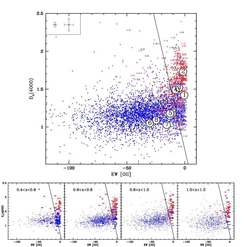
In figure 4 (top panel) the relation between the equivalent width of the [OII]$\lambda$3727 line (EW[OII]) and the 4000 Å break (D4000) is shown for the whole “spectroscopic sub-sample”. Blue symbols are objects with $U-V<1.0$, while red symbols are objects with $U-V>1.0$. It is clearly visible from the plot how objects follow a bimodal L-shaped distribution, with most of the star-forming objects that have a large EW[OII] having a negligible D4000, and vice-versa most of the objects that have a strong D4000 showing no significant [OII] emission in their spectra. The bottom panels of figure 4, obtained dividing the “spectroscopic sub-sample” in four redshit bins, show that this bimodality is essentially independent from redshift. The larger dispersion in the D4000 measurements of star-forming objects in the higher redshift bin is mostly due to the higher uncertainties in measuring this feature for distant and faint objects.

These distributions suggest a natural sub-division of the galaxy population into two classes. We define spectral early-type objects (ET) galaxies in the vertical arm of the two parameters distribution, i.e. those that do not show any detectable sign of star formation activity, and which can be expected to undergo further evolution only via passive evolution of their stellar population. Conversely, we define spectral late-type objects (LT) galaxies in the horizontal arm, still undergoing a vigorous star formation activity. More elaborated spectral classification schemes have been proposed in the past, like the four-fold subdivision discussed by Mignoli et al. (2005), but we prefer to use here a simpler two-fold subdivision, that mirrors the one obtained using the rest-frame colors.

Figure 5: a) U-V rest-frame color distribution; the shaded histogram is for the LT population, while the heavy line histogram is for the ET population. The inset shows the same histograms drawn only for the higher S/N objects. b) U-V vs V color-magnitude relation; filled dots are ET objects, tiny dots are LT ones. Both plots include only the objects with redshift within the interval 0.6-0.8 from the “spectroscopic sub-sample”

To a first approximation the definition of the separating boundary between LT and ET galaxies in the D4000 vs. EW[OII] parameters space could be a vertical line at EW[OII]=10Å , the approximate detection limit for the [OII] line in our data. This definition, however, would lead us to include many objects with very low D4000 and a real, albeit undetected, [OII] emission in the ET sample, which is obviously contrary to the natural definition of early-type galaxies as objects with an evolved stellar population (large D4000; see Kauffmann et al. 2003b) and no current star formation activity (no [OII] emission line). To alleviate this problem, we have checked various definitions of the ET-LT separating boundary line that would keep constant the ratio of ET to LT galaxies. We have built a composite spectrum of the ET population for each one of the definitions so that the higher signal-to-noise ratio thus achieved would allow a robust measurement of the [OII] emission at fainter intensities. Then we have selected the subdivision that minimizes the equivalent width of the [OII] line in the composite spectrum of the resulting ET population. This optimization procedure results in a slightly tilted boundary line described by the relation:

$D_{n}(4000)+EW([OII])/15.0=0.7$

According to this definition, ET galaxies have $D_{n}(4000)+EW([OII])/15.0$ above 0.7, while LT galaxies are below that value. Purely for comparison, in figure 4 we have also plotted as large numbered circles the $D_{n}(4000)$ and $EW([OII])$ values measured on Virgo cluster templates from Gavazzi et al. (2002). Table 3 recaps the legend for the circles. It should not be surprising that our ET-LT boundary is including early spirals within the ET population, and only Sc and later types within the LT population. This is a rather general property of classification schemes based on galaxy color or spectral properties. For example, the earliest spiral galaxy SED presented by Coleman et al. (1980) is that typical of Sbc galaxies, and this same SED was used by Lilly et al. (1995) to separate red and blue galaxies in their CFRS galaxy sample. Similarly, the earliest spiral galaxy color-color track used by Adelberger et al. (2004) in defining the color selection criteria for isolating star-forming galaxies in the redshift range $1<z<3$ is that typical of an Sb galaxy.

We consider this spectral classification as a better substitute for a true morphological classification with respect to color for a number of reasons: it is based on directly measurable quantities and avoids the uncertainties involved in estimating rest-frame colors; it is directly based on two important physical properties like the age of the stellar population and the amount of star formation activity taking place in each galaxy; unlike colors, it is minimally affected by the unknown amount of reddening inside each galaxy. One possible limitation affecting our spectral classification is the fact that a number of objects with relatively young stellar population, as witnessed by the small value of their D4000, is included within the ET population. However we prefer not to exclude these objects by some modification of the ET-LT separation boundary, because any such a modification would make our classification scheme much more vulnerable to progenitor bias effects (van Dokkum & Franx 2001). With the current scheme as soon as a galaxy has completed the bulk of its star formation activity and is starting the purely passive evolution phase it becomes an ET object, and it remains such at all subsequent times, as its stellar population ages and the D4000 amplitude in its spectrum increases. Instead, any significant star formation activity would move an object towards the left in the figure 4 diagram, effectively removing it from the ET population. This minimization of progenitor bias effects on our classification scheme is the main reason we can use a redshift-independent classification scheme in our analysis.

5.2 The contamination effect

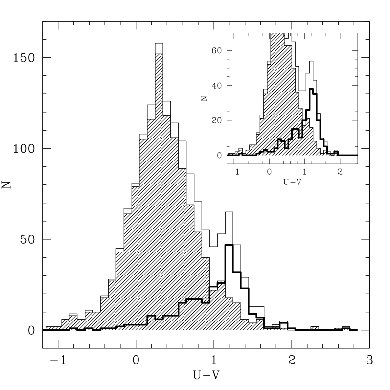
Having obtained an early- vs. late-type galaxy separation based on spectral properties, we analyse what is the color distribution of these two categories, and compare this spectral classification with the “red-peak” color one. Figure 5a shows the global U-V rest-frame color distribution for our “spectroscopic sub-sample” in the redshift interval where the peak of the N(z) distribution is located ($0.6<z<0.8$, see Le Fèvre et al. 2005). In this paragraph we focus our analysis on this redshift bin before extending it to the whole redshift range to study the evolution of the contamination.

The shaded histogram represents the color distribution for the LT objects, while the thick line shows the distribution for the ET population. The thin line histogram represents the sum of the two distributions. As expected, the red peak of the global color distribution is mainly populated by ET objects, while the blue peak is mainly populated by LT ones, but a rather strong contamination between the two populations is present. The inset plotted in figure 5a shows the same histograms drawn considering only the objects with higher S/N spectra (2229 objects); it is easy to see how very little difference is observed when removing low S/N spectra objects, for which spectral feature measurements are more uncertain. We therefore conclude that uncertainties in the spectral classification are not the primary source for the significant overlap in color space between the two populations. The color distributions for the two populations have a very significant overlap at intermediate colors, and a simple color cut is not able to separate the galaxy populations according to the spectral classification defined above. In other words, a purely color based classification does not completely account for the different stellar populations and star formation history properties.

Figure 6: The “contamination” effect in the redshift range $0.6<z<0.8$. The fraction of the whole ET population which is included in the resulting RED population (lower panel) and the “contamination” of the resulting RED sample (upper panel) as a function of the limiting color used to define it.

Similar results have been obtained by Bundy et al. (2005) using the DEEP2 data (see their figure 1), although they use a different color and a slightly different criterion for their spectral classification of passive and star-forming galaxies. The same contamination effect is visible in the color-magnitude relation plot (figure 5b). Projecting the color-magnitude relation along the slope of the red sequence to obtain “corrected” color histograms, as done for example in B04, does not significantly change the situation.

From the total histogram in figure 5 we see that a purely color-based definition of the red peak population (hereafter RED population) would be that of galaxies with $U-V>1.0$, in agreement with the color cut implemented by B04. This is the color where a local minimum is observed in the color distribution, and it is also the color at which we observe the transition from an LT dominated population to an ET dominated one. However, because of the significant color overlap between the two populations, it is clear that the resulting RED population includes not only ET (i.e. really passive) objects, but also a significant fraction of LT (i.e. star-forming) ones. Moreover this RED population does not include a significant fraction of ET objects which have bluer colors.

In figure 6 we quantify such “contamination”. The lower panel shows, as a function of the color cut we use to define the RED population, the fraction of the whole ET population which is included in it. The upper panel shows, on the contrary, the “contamination” of the resulting RED sample, i.e. which percentage of the total RED population is actually composed of LT objects.

Error bars in this and the following two figures have been computed using simple Montecarlo simulations. The main sources of uncertainty, beside the Poissonian error on population counts, are the uncertainties on the spectroscopic and photometric measurements. In our simulations we generated mock datasets by adding to the measured values random offsets, generated from a Gaussian distribution characterized by a $\sigma$ equal to the measurement uncertainty for the given quantity. Then we repeated our determinations of the contamination effect for all the mock datasets to obtain an estimate for standard deviation of each data point in the plots.

To these Montecarlo uncertainty estimates we have also added the appropriate Poissonian counting uncertainties. The small values for the contamination uncertainties demonstrate that the effect we are witnessing is real, and not the result of some bias introduced by measurement uncertainties. Using the $U-V>1.0$ cut we include in the RED population only $\sim 60\%$ of the ET objects, the remaining $\sim 40\%$ having bluer colors. At the same time, 35% of our RED population will be actually constituted by LT objects which have red colors, but show clear spectroscopic indication of star formation activity.

To summarize, 65% of our RED population are ET population (and these objects are 60% of all the ET objects) while 35% are LT objects.

As shown in section 2.2.2 a small fraction of photometric early-type objects is missing in the spectroscopic sample due to the lower efficiency in measuring the redshift for these galaxies with respect to the late-type ones. However, this fraction is small and it does not change the reliability of our results; adding a few percents of objects in the red peak would not change significantly the observed contamination, even if all the “new” red objects were to be ET objects. We therefore consider the bias introduced by the lower redshift measurement efficiency to be almost negligible.

5.3 Contamination evolution with redshift

Figure 7: The fraction of the ET objects which are included in the RED population and the corresponding LT contamination computed for a limiting color $U-V=1.0$ as a function of redshift. The solid line is for the whole “spectroscopic sub-sample”; the dashed line is computed using only objects brighter than $M_{V}=-20$.

The contamination effect changes somewhat with redshift as shown in figure 7 (solid line). The definition of the RED population at different redshifts is derived from the color distributions shown in figure 1, where a local minimum in the distributions is located at $\sim U-V=1.0$ for all redshift bins (within the small uncertainty introduced by the arbitrary binning of the data). We therefore define as RED galaxies all objects with color $U-V>1.0$ within all our redshift bins.

The fraction of RED ET objects shows little evolution over most of the redshift range we cover with our sample, while the RED objects LT contamination becomes more important with redshift as could be expected because of the well known widespread increase in star formation activity from the local universe to redshift 1-2 that should results in a higher contaminating fraction of dusty starburst galaxies in the RED population.

One exception is represented by the low fraction of ET objects observed in the lowermost redshift bin, but this result is significantly affected by our sample characteristics. The first effect is due to the VVDS relatively small field of view; the number of bright objects we have in the lowest redshift bins is small, and since these bright objects are predominantly red galaxies, this results in a smaller fraction of ET galaxies included in the red sample. Moreover in the lowest redshift bins we include faint objects which are not observable at higher redshift. As already discussed by Kaviraj et al. (2006), we observe that the type mix in the RED population depends on the range of galaxy luminosities that are included in the sample.

By restricting ourselves only to galaxies brighter than $M_{V}=-20$ (dashed line in figure 7) we observe a much smaller evolution with redshift of the RED ET fraction, and a somewhat smaller contamination from LT objects. Although some of these differences could be due to larger errors in the measurements of photometric and spectroscopic parameters for the fainter objects, we clearly observe that transition objects (blue ET or red LT galaxies) are found preferentially at fainter luminosities.

Figure 8: In the upper panel the distribution of star formation rates for the contaminating LT population among the RED galaxies is shown. The evolution of the median value with redshift is plotted in the lower panel. The solid line is the SSFR which is required to double the galaxy stellar mass between the given redshift and the present time, which discriminates between quiescent and strongly star-forming galaxies.

To quantify how different from a passively evolving object is the typical contaminant galaxy, we have derived current specific star formation rate estimates for all the RED population LT galaxies, using the [OII] luminosity conversion factor given by Kennicutt (1998). The resulting distribution of specific star formation rates is shown in the upper panel of figure 8 and has a median value of $6.76\times 10^{-10}\leavevmode\nobreak\ yr^{-1}$. The lower panel of figure 8 shows the evolution of the median value with redshift. The solid line in this plot represents the SSFR which is required to double the galaxy stellar mass between the given redshift and the present time, assuming a constant SFR; this “doubling” SSFR is used to discriminate between quiescent and star-forming galaxies. It is easy to see that, at all redshifts, the median SSFR value is above the threshold. It is clear that a significant number of dusty starburst galaxies is included in the RED population, and its presence should be accounted for in studying the evolution of the RED population properties. This result is in agreement with the findings of Giallongo et al. (2005), who found some 35% of dusty starburst objects within the red population of their HDF N+S sample, and with those of Cassata et al. (2007), who found a similar fraction of 33% edge-on spirals within their sample of red galaxies in the COSMOS survey field. We also notice that the luminosity dependence of the observed LT contamination brings our results in agreement with the findings of Bell et al. (2004a) who measured a contamination of some 15% from morphologically classified late-type galaxies in their bright red galaxies sample. In a similar redshift bin, using a similar sample (our bright sample limited to $M_{V}<-20$), we measure a contamination from LT objects which is between 13 and 21 percent (see figure 7, dashed line).

Figure 9: The fraction of the ET objects which are included in the RED population and the corresponding LT contamination computed for multi-color types (see section 5.4). The solid line is for the whole “spectroscopic sub-sample”; the dashed line is computed using only objects brighter than $M_{V}=-20$.

5.4 The multi-color type approach

Given the not entirely satisfactory results obtained by a pure color selection in isolating an old, passively evolving galaxy population, we have considered also an alternative approach towards this goal, still based solely on photometric data, using the “photometric type” classification scheme described in section 2.2.2.

This approach does not account for any global SED variation over cosmic time as a result of the evolution of the stellar populations, nor for the effects of a progenitor bias (van Dokkum & Franx 2001) against the early-type galaxy population. Still, it provides a very simple and model-independent “no evolution” reference for any other, more complex modeling of galaxy populations evolution.

Figure 9 shows the fraction of the ET objects which are included in the “photometric early-type population” and the corresponding LT contamination computed for multi-color types. Comparing figure 7 with figure 9 we see that, the multi-color type approach has a somewhat higher efficiency in separating old passive galaxies from star forming ones. Indeed with the single $U-V$ color separation we isolate on average (over the redshift range covered by our sample) about 60% of the ET galaxies, whereas in the case of the multi-color separation this fraction is $\sim$ 70%. We note that the 35% level of LT contamination is similar in both cases. Also the trends with redshift of both the fractions of selected ET galaxies and of LT galaxies contamination are comparable to the single color approach, since in both cases the selection criterion does not evolve with redshift.

Given the above results, we conclude that the photometric types approach is to be preferred to the color selection one, as it provides a finer degree of subdivision between galaxy properties than the color separation, making it a better tool for the study of galaxy evolution. Again, like in the case of the color selection, we observe a luminosity dependence for the population mix; limiting our sample to the bright $M_{B}<-20$ objects we observe a smaller evolution with redshift of the RED ET fraction, and a somewhat smaller contamination from LT objects.

6 The CMR of the spectral early-type population

Figure 10: Color evolution for four classes of objects as measured by the value of the intercept of the CMR at $M_{V}=-20$. Small filled circles are the VVDS color selected data (as in figure 3); open triangles are the photometric early-type population; filled squares are the ET population; open circles are the “oldest” part of the ET population, i.e. the ET objects for which the value of the D_n(4000) is higher than 1.45. The lowermost redshift point for the spectroscopical ET sample is plotted also considering only objects brighter than $M_{V}=-20$ (big filled square)

In section 4 we have analyzed the properties of the CMR of color-selected early-type galaxies in our sample, showing that there is a generally good agreement between the observed evolution of the CMR and the expectations for a purely passively evolving population. Having shown that a very significant contamination of the red population from (presumably dust-reddened) actively star-forming galaxies is present, we must consider the possibility that the above agreement is in fact a rather fortuitous one.

In figure 10 we now plot the evolution of the CMR for the spectroscopically selected ET galaxies (filled squares), and also for the multi-color selected early-type ones (open triangles). Notice how the lowermost redshift point for the spectroscopically defined ET sample is abnormally blue, in agreement with the small fraction of RED ET galaxies shown in figure 7 for the same redshift bin. If we consider once again only objects brighter than $M_{V}=-20$, the point moves to a significantly redder color (as shown in the figure by the big filled square).

From a comparison with figure 3 we can see that only small differences are present in the CMR of the different early-type samples (the solid circles in this figure are the same as in figure 3, representing the evolution of the CMR for the color-selected red galaxies). The color-magnitude relations of ET and multi-color selected early-type galaxies are on average 0.15 magnitudes bluer than that of red galaxies, as could be expected from the presence of a blue color tail in these galaxy samples. Even restricting the ET sample to the “oldest” part of the ET population, i.e. the ET objects for which the value of the D_n(4000) is higher than 1.45 (open circles in figure 10) does not change very significantly the situation, although the CMR for these objects is slightly redder than that of the full ET sample.

The single-color, multi-color, and spectroscopically selected samples of early-type galaxies we have obtained are not independent, having some 60% of galaxies in common, and therefore a certain degree of similarity in the various color-magnitude relations we have derived is expected. But we see from figure 10 how the red sample, including some 40% contamination from actively star-forming galaxies, and the subset of the “oldest” ET galaxies, composed almost exclusively by galaxies with an old stellar population and no current star-formation activity, are described by essentially the same CMR, over a rather large redshift interval. These findings support the conclusion that the average color of the red objects, as measured by the CMR value at fixed luminosity, may not be a very sensitive indicator for measuring the evolution of the early-type galaxy population.

This important issue deserves a more extended analysis. In future papers we will study the spectral classification in more detail and expand our analysis on the effects that different sample selection criteria can have on the inferred properties of the early- and late-type galaxy populations.

7 Summary and conclusions

In this paper we have conducted the study of the rest-frame color distributions on a sample of 6291 galaxies from the first epoch VVDS.

We find that the well-studied local bimodal distribution is still present at previously unexplored redshifts up to at least z=1.5 (the mean redshift for the galaxies in the redshift bin $1.2<z<2.0$).

Given the large interval of redshift and luminosity spanned by our sample, we were able to study also the dependence of rest-frame colors distributions on these quantities. We have shown how, at each redshift, faint galaxies are bluer than the luminous ones. Moreover, at any given luminosity, galaxies become bluer as redshift increases and the amount of this effect is quite independent on the luminosity. This result extends for the first time the findings of previous redshift surveys significantly over the $z\approx 1$ limit. We have extended up to $z\sim 2$ the results of B04 about the evolution of the CMR of red galaxies, finding a slightly smaller evolution and a better agreement with the $z=0$ point.

We have analyzed the galaxy population which constitutes the red-peak of the color distributions finding that a significant fraction is composed of star forming objects. The detailed quantification of this effect at various redshifts proves how a simple color selection is not able to reliably isolate early-type objects. The different approach used within the VVDS to isolate galaxy types, based solely on photometric data and local spectral templates fitting, has been shown to have a slightly better capability of isolating passive object than that based on a single color.

Using a robust spectral classification of early-type galaxies in the D_n(4000)/EW([OII]) plane, we have demonstrated that a population of galaxies selected only on the basis of their red colors is not only including early-type galaxies with little star formation, but also a significant contamination by star-forming galaxies. We conclude that there is no one to one correspondence between red-sequence and ”dead and old” galaxies, and that selecting galaxies only on the basis of their colors can be misleading in estimating the evolution of old and passively evolving galaxies.

References

- Adelberger et al. (2004) Adelberger, K. L., Steidel, C. C., Shapley, A. E., et al. 2004, ApJ, 607, 226
- Baldry et al. (2004a) Baldry, I. K., Balogh, M. L., Bower, R., Glazebrook, K., & Nichol, R. C. 2004a, in AIP Conf. Proc. 743: The New Cosmology: Conference on Strings and Cosmology, 106–119
- Baldry et al. (2004b) Baldry, I. K., Glazebrook, K., Brinkmann, J., et al. 2004b, ApJ, 600, 681
- Balogh et al. (2004) Balogh, M., Eke, V., Miller, C., et al. 2004, MNRAS, 348, 1355
- Balogh et al. (1999) Balogh, M. L., Morris, S. L., Yee, H. K. C., Carlberg, R. G., & Ellingson, E. 1999, ApJ, 527, 54
- Beers et al. (1990) Beers, T. C., Flynn, K., & Gebhardt, K. 1990, AJ, 100, 32
- Bell et al. (2004a) Bell, E. F., McIntosh, D. H., Barden, M., et al. 2004a, ApJ, 600, L11
- Bell et al. (2004b) Bell, E. F., Wolf, C., Meisenheimer, K., et al. 2004b, ApJ, 608, 752
- Bernardi et al. (2003) Bernardi, M., Sheth, R. K., Annis, J., et al. 2003, AJ, 125, 1882
- Bottini et al. (2005) Bottini, D., Garilli, B., Maccagni, D., et al. 2005, PASP, 117, 996
- Bower et al. (1992) Bower, R. G., Lucey, J. R., & Ellis, R. S. 1992, MNRAS, 254, 601
- Brinchmann et al. (2004) Brinchmann, J., Charlot, S., White, S. D. M., et al. 2004, MNRAS, 351, 1151
- Bruzual (1983) Bruzual, G. 1983, ApJ, 273, 105
- Bruzual & Charlot (2003) Bruzual, G. & Charlot, S. 2003, MNRAS, 344, 1000
- Budavári et al. (2003) Budavári, T., Connolly, A. J., Szalay, A. S., et al. 2003, ApJ, 595, 59
- Bundy et al. (2005) Bundy, K., Ellis, R. S., Conselice, C. J., et al. 2005, American Astronomical Society Meeting Abstracts, 207,
- Cassata et al. (2007) Cassata, P., Guzzo, L., Franceschini, A., et al. 2007, astro-ph/0701483
- Cimatti et al. (2002) Cimatti, A., Daddi, E., Mignoli, M., et al. 2002, A&A, 381, L68
- Coleman et al. (1980) Coleman, G. D., Wu, C.-C., & Weedman, D. W. 1980, ApJS, 43, 393
- Cowie et al. (1996) Cowie, L. L., Songaila, A., Hu, E. M., & Cohen, J. G. 1996, AJ, 112, 839
- Cucciati et al. (2006) Cucciati, O., Iovino, A., Marinoni, C., et al. 2006, A&A, 458, 39
- Dekel & Birnboim (2006) Dekel, A. & Birnboim, Y. 2006, MNRAS, 368, 2
- Dressler (1980) Dressler, A. 1980, ApJ, 236, 351
- Gavazzi et al. (2002) Gavazzi, G., Bonfanti, C., Sanvito, G., Boselli, A., & Scodeggio, M. 2002, ApJ, 576, 135
- Gavazzi et al. (2003) Gavazzi, G., Boselli, A., Donati, A., Franzetti, P., & Scodeggio, M. 2003, A&A, 400, 451
- Gavazzi et al. (1996) Gavazzi, G., Pierini, D., & Boselli, A. 1996, A&A, 312, 397
- Giallongo et al. (2005) Giallongo, E., Salimbeni, S., Menci, N., et al. 2005, ApJ, 622, 116
- Ilbert et al. (2006) Ilbert, O., Arnouts, S., McCracken, H. J., et al. 2006, A&A, 457, 841
- Ilbert et al. (2004) Ilbert, O., Tresse, L., Arnouts, S., et al. 2004, MNRAS, 351, 541
- Ilbert et al. (2005) Ilbert, O., Tresse, L., Zucca, E., et al. 2005, A&A, 439, 863
- Kauffmann et al. (2003a) Kauffmann, G., Heckman, T. M., White, S. D. M., et al. 2003a, MNRAS, 341, 33
- Kauffmann et al. (2003b) Kauffmann, G., Heckman, T. M., White, S. D. M., et al. 2003b, MNRAS, 341, 54
- Kaviraj et al. (2006) Kaviraj, S., Devriendt, E. G., Ferreras, I., Yi, S. K., & Silk, J. 2006, astro-ph/0602347
- Kennicutt (1998) Kennicutt, R. C. 1998, ARA&A, 36, 189
- Kodama & Arimoto (1997) Kodama, T. & Arimoto, N. 1997, A&A, 320, 41
- Kodama et al. (1999) Kodama, T., Bower, R. G., & Bell, E. F. 1999, MNRAS, 306, 561
- Le Fèvre et al. (2004) Le Fèvre, O., Mellier, Y., McCracken, H. J., et al. 2004, A&A, 417, 839
- Le Fèvre et al. (2005) Le Fèvre, O., Vettolani, G., Garilli, B., et al. 2005, A&A, 439, 845
- LeFevre et al. (2003) LeFevre, O., Saisse, M., Mancini, D., et al. 2003, in Instrument Design and Performance for Optical/Infrared Ground-based Telescopes. Edited by Iye, Masanori; Moorwood, Alan F. M. Proceedings of the SPIE, Volume 4841, pp. 1670-1681 (2003)., ed. M. Iye & A. F. M. Moorwood, 1670–1681
- Lilly et al. (1995) Lilly, S. J., Tresse, L., Hammer, F., Crampton, D., & Le Fèvre, O. 1995, ApJ, 455, 108
- McCracken et al. (2003) McCracken, H. J., Radovich, M., Bertin, E., et al. 2003, A&A, 410, 17
- Menci et al. (2005) Menci, N., Fontana, A., Giallongo, E., & Salimbeni, S. 2005, ApJ, 632, 49
- Meneux et al. (2006) Meneux, B., Le Fèvre, O., Guzzo, L., et al. 2006, A&A, 452, 387
- Mignoli et al. (2005) Mignoli, M., Cimatti, A., Zamorani, G., et al. 2005, A&A, 437, 883
- Radovich et al. (2004) Radovich, M., Arnaboldi, M., Ripepi, V., et al. 2004, A&A, 417, 51
- Renzini (2006) Renzini, A. 2006, ARA&A, 44, 141
- Roberts & Haynes (1994) Roberts, M. S. & Haynes, M. P. 1994, ARA&A, 32, 115
- Salpeter (1955) Salpeter, E. E. 1955, ApJ, 121, 161
- Sandage (1986) Sandage, A. 1986, A&A, 161, 89
- Schlegel et al. (1998) Schlegel, D. J., Finkbeiner, D. P., & Davis, M. 1998, ApJ, 500, 525
- Scodeggio et al. (2005) Scodeggio, M., Franzetti, P., Garilli, B., et al. 2005, PASP, 117, 1284
- Stanford et al. (1998) Stanford, S. A., Eisenhardt, P. R., & Dickinson, M. 1998, ApJ, 492, 461
- Strateva et al. (2001) Strateva, I., Ivezić, Ž., Knapp, G. R., et al. 2001, AJ, 122, 1861
- Tremonti et al. (2004) Tremonti, C. A., Heckman, T. M., Kauffmann, G., et al. 2004, ApJ, 613, 898
- Tully et al. (1982) Tully, R. B., Mould, J. R., & Aaronson, M. 1982, ApJ, 257, 527
- van Dokkum & Franx (2001) van Dokkum, P. G. & Franx, M. 2001, ApJ, 553, 90
- Visvanathan & Sandage (1977) Visvanathan, N. & Sandage, A. 1977, ApJ, 216, 214
- Weiner et al. (2005) Weiner, B. J., Phillips, A. C., Faber, S. M., et al. 2005, ApJ, 620, 595
- Zanichelli et al. (2005) Zanichelli, A., Garilli, B., Scodeggio, M., et al. 2005, PASP, 117, 1271
- Zucca et al. (2006) Zucca, E., Ilbert, O., Bardelli, S., et al. 2006, A&A, 455, 879