The oxygen abundance calibrations and N/O abundance ratios of $\sim$ 40,000 SDSS star-forming galaxies

Abstract

Using a large sample of 38,478 star-forming galaxies selected from the Second Data Release of the Sloan Digital Sky Survey database (SDSS-DR2), we derive analytical calibrations for oxygen abundances from several metallicity-sensitive emission-line ratios: [N ii]/H$\alpha$, [O iii]/[N ii], [N ii]/[O ii], [N ii]/[S ii], [S ii]/H$\alpha$, and [O iii]/H$\beta$. This consistent set of strong-line oxygen abundance calibrations will be useful for future abundance studies. Among these calibrations, [N ii]/[O ii] is the best for metal-rich galaxies due to its independence on ionization parameter and low scatter. Dust extinction must be considered properly at first. These calibrations are more suitable for metal-rich galaxies (8.4$<$12+log(O/H)$<$9.3), and for the nuclear regions of galaxies. The observed relations are consistent with those expected from the photoionization models of Kewley & Dopita (2002). However, most of the observational data spread in a range of ionization parameter $q$ from $1\times 10^{7}$ to $8\times 10^{7}$ cm s^-1, corresponding to log$U$=$-$3.5 to $-$2.5, narrower than that suggested by the models. We also estimate the (N/O) abundance ratios of this large sample of galaxies, and these are consistent with the combination of a “primary” and a dominant “secondary” components of nitrogen.

1. Introduction

The chemical properties of stars and gas within a galaxy are a fossil record chronicling its history of star formation. Optical emission lines from H ii regions have long been the primary means of gas-phase chemical diagnostics in galaxies (Aller 1942; Searle 1971; reviews by Peimbert 1975; Pagel 1986; Shields 1990; Aller 1990; Peimbert, Rayo, & Torres-Peimbert 1975; Osterbrock 1989; de Robertis 1987). Osterbrock (1989) thoroughly discusses the standard techniques for measuring the chemical properties of ionized gas, which require measurements of H and He recombination lines along with collisionally excited lines from one or more ionization states of heavy element species.

Oxygen is the most commonly used metallicity indicator in the interstellar medium (ISM) by virtue of its relatively high abundance and strong emission lines in the optical region of the spectrum (e.g., [O ii]$\lambda$ 3727 and [O iii]$\lambda$$\lambda$4959, 5007). Ideally, the oxygen abundance is measured directly from ionic abundances obtained through a determination of the electron temperature ($T_{e}$) of the H ii region. This is known as the “$T_{e}-$method” (Pagel et al. 1992; Skillman & Kennicutt 1993). The ratio of a high-excitation auroral line such as [O iii]$\lambda$4363 to the lower excitation [O iii]$\lambda$$\lambda$4959,5007 lines provides a direct measurement of the electron temperature in the physical medium where O⁺⁺ is the dominant ionization state. However, [O iii]$\lambda$4363 is only prominent in metal-poor H ii regions. In most cases, where [O iii]$\lambda$4363 is too weak to be detected, metallicities of H ii regions have to be estimated from “strong-line” ratios. A commonly used one is $R_{23}$:

$$R_{23}=\frac{f([\mathrm{OIII}]\lambda\lambda 4959,5007)+f([\mathrm{OII]\lambda\lambda 3726,3729)}}{f(\mathrm{H\beta)}}.$$ (1)

Many calibrations of converting $R_{23}$ to 12+log(O/H) abundance have been published, including Pagel et al. (1979), Pagel, Edmunds, & Smith (1980), Edmunds & Pagel (1984), McCall, Rybski, & Shields (1985), Dopita & Evans (1986), Torres-Peimbert, Peimbert, & Fierro (1989), Skillman, Kennicutt, & Hodge (1989), McGaugh (1991), Zaritsky, Kennicutt, & Huchra (1994), Kobulnicky et al. (1999, K99), Pilyugin (2000, 2001a,b), Tremonti et al. (2004, T04), Salzer et al. (2005) and Kewley & Dopita (2002) (hereafter KD02) etc. Some calibrations have attempted to take the ionization parameters into account (e.g., McGaugh 1991; KD02 etc.), but others have not. However, one problem is that the relationship between $R_{23}$ and 12+log(O/H) is double valued, with the transition between the upper metal-rich branch and the lower metal-poor branch occurring near 12+log(O/H)$\sim$8.4 (log$R_{23}$$\sim$0.8). Moreover, in many cases $R_{23}$ is unavailable due to the limit of wavelength coverage or the poor quality around one or some of the related lines. One can then use other various metallicity-sensitive strong-line ratios to estimate metallicities of galaxies, including [N ii]$\lambda$6583/H$\alpha$, [O iii]$\lambda$5007/[N ii]$\lambda$6583, [N ii]$\lambda$6583/[O ii]$\lambda$3727, [N ii]$\lambda$6583/[S ii]$\lambda$$\lambda$6717,6731, [S ii]$\lambda$$\lambda$6717,6731/H$\alpha$, and [O iii]$\lambda$$\lambda$4959,5007/H$\beta$. Even when $R_{23}$ is available, these ratios are also useful for breaking the $R_{23}$ upper/lower branch degeneracy. We should notice that some of these strong-line ratios are also sensitive to interstellar reddening (e.g. N ii]/[O ii]) or depend on the ionization parameter.

Some researchers have used $T_{e}$-based abundance data to calibrate for some of these strong-line ratios, for example, Denicoló et al. (2002) obtained a linear calibration of [N  ii]/H$\alpha$ to 12+log(O/H) from a combined sample of 108 metal-poor galaxies with [O iii]4363 detected and 128 metal-rich galaxies; Pettini & Pagel (2004) studied the calibration relations between [N ii]/H$\alpha$, ([O iii]/H$\beta$ )/([N ii]/H$\alpha$) and 12+log(O/H) from 137 galaxies with $T_{e}$ -derived O/H abundances (including six of them from photoionization models). Pérez-Montero & Díaz (2005) also studied some calibrations from the collected 367 emission-line objects on the basis of the $T_{e}$-based oxygen abundances, but they did not derive analytic calibrating relations. However, these observations are limited to modest samples, and only apply to some of the strong-line ratios. The much larger consistent data set (several tens of thousands) from the recently released SDSS database could provide much more information about many of the strong-line ratio calibrations for metallicities of galaxies.

KD02 used a combination of stellar population synthesis and photoionization models to calibrate several strong-line abundance diagnostics. In the KD02 models, strong line ratios are a function of both metallicity and ionization parameter. The ionization parameter, $q$, is a measure of the number of ionizing photons per atom at the inner boundary of the nebula. To determine both metallicity and ionization parameter, KD02 suggested a somewhat complicated iterative approach involving a number of line ratios. We advocate a simpler approach in this study. In Sect. 4 we compare the observed line ratios of a large sample of star-forming galaxies selected from the SDSS-DR2 to the predictions of the KD02 models and show that galaxies span a smaller range of $q$ than used by KD02. We therefore ignore any explicit dependence of the line ratios on $q$, and use observational data to derive strong-line abundance calibrations which reflect the mean ionization parameter of the data at a given metallicity.

The SDSS-DR2 database is very well suited for this kind of study. There are a large number of galaxies at any given value of oxygen abundance between about 8.4 and 9.3, which makes it ideal for measuring correlations between metallicity and various strong-line ratios and for quantifying the scatter. We make use of the emission line data and metallicities described in Brinchmann et al. (2004) and Tremonti et al. (2004) which have been made publicly available on the web. The oxygen abundances presented in Tremonti et al. (2004) were derived using Bayesian techniques to compare multiple strong emission lines to a grid of photoionization models (Charlot et al. 2006). We use the $R_{23}$ metallicity calibration of Tremonti et al. to derive a fiducial oxygen abundance. We then examine correlations between the oxygen abundances and the observed several strong emission-line ratios: [N ii]/H$\alpha$, [O iii]/[N ii], [N ii]/[O ii], [N ii ]/[S ii], [S ii]/H$\alpha$, and [O iii]/H$\beta$, then derive new strong-line metallicity calibrations where appropriate. Our approach differs from the usual way in which abundance indicators are calibrated: 1) using samples of galaxies with direct ($T_{e}$-based) abundances (e.g. Pagel et al. 1979; Pettini & Pagel 2004); 2) using photoionization model grids (e.g. McGaugh 1991; Charlot & Longhetti 2001; KD02). Our calibrations are valid for high metallicity (12+log(O/H) $>$ 8.4) galaxies, where the $T_{e}$-based abundances are only available for a handful of objects (Bresolin et al. 2004, 2005; Garnett et al. 2004a,b). We note that our calibrations may be subject to the same systematic uncertainty as the models. For comparison, we use the $R_{23}$ calibration of McGaugh (1991) (as Kobulnicky et al. 1999) to derive the fiducial metallicities as well.

We also estimate the log(N/O) abundance ratios of these sample galaxies by using the algorithm given by Thurston et al. (1996), including the estimated temperature in the [N  ii] emission regions. This will be the first such large sample for the observed log(N/O) abundances, and will be useful for understanding the “primary” or “secondary” origin of nitrogen. Specially, the strength of the SDSS dataset is that there are a large number of galaxies at any given value of oxygen abundance between about 8.4 and 9.3. This makes it ideal for quantifying the scatter in various trends.

This paper is organized as follows: the sample selection and $R_{23}$ -derived oxygen abundances are described in Sect.2; Sect.3 shows the derived calibrations of the linear and/or third-order polynomial fits from the observational relations of 12+log(O/H) versus the various strong emission-line ratios; these observational relations are compared with the photoionization models of KD02 in Sect.4; The log(N/O) abundance ratios of the sample galaxies are given in Sect.5; and we conclude in Sect.6.

2. Sample selection, and R₂₃-derived oxygen abundances

The data analyzed in this study are drawn from the SDSS-DR2 (Abazajian et al. 2004). These galaxies are part of the SDSS “main” galaxy sample used for large-scale structure studies (Strauss et al. 2002). We select the sample galaxies having Petrosian r magnitudes in the range 14.5$<r<$17.77 mag after correction for foreground Galactic extinction using the reddening maps of Schlegel et al. (1998), which yields 193,890 objects from the total of 261,054 objects.

We only consider galaxies whose metallicities have been estimated by Tremonti et al. (2004), leaving 50,385 galaxies. They selected star-forming galaxies using the criteria given by Kauffmann et al. (2003b) following the traditional line diagnostic diagram of [N ii]/H$\alpha$ vs. [O iii]/H$\beta$ which has been used by Baldwin, Phillips, Terlevich (1981, BPT), Veilleux & Osterbrock (1987) and Kewley et al. (2001) etc.

Tremonti et al. (2004) discussed the weak effect of the 3^′′ aperture of the SDSS spectroscopy on estimated metallicities of the sample galaxies with redshifts $0.03<z<0.25$. Kewley et al. (2005) further recommended that, to get reliable metallicities, redshifts $z>0.04$ are required for the SDSS galaxies to ensure a covering fraction $>$20% of the galaxy light. Thus, we select the galaxies with redshifts $0.04<z<0.25$, which then leaves 40,693 objects.

We only consider the objects for which fluxes have been measured for [O  ii], H$\beta$, [O iii], H$\alpha$, [N ii] (also [S ii] in the study in Sects. 3.5, 3.6). It leaves 40,293 objects (39,919 if the [S ii]6717,6731 are included to be considered as well). Also, the sample objects should have higher S/N ratios by requiring them to have lines of H$\beta$, H $\alpha$, and [N ii]6583 detected at greater than 5$\sigma$. It leaves 39,029 objects.

The oxygen abundances of the sample galaxies were estimated using the $R_{23}$ method. The emission-line fluxes must first be corrected for dust extinction. The extinction correction of the sample galaxies are derived using the Balmer line ratio H$\alpha$/H$\beta$: assuming case B recombination, with a density of 100 cm^-3 and a temperature of 10⁴ K, and the predicted intrinsic ratio of H$\alpha$/H$\beta$ is 2.86 (Osterbrock 1989), with the relation of

$$(\frac{I_{H\alpha}}{I_{H\beta}})_{obs}=(\frac{I_{H\alpha_{0}}}{I_{H\beta_{0}}})_{intr}10^{-c(f(H\alpha)-f(H\beta))}.$$ (2)

Using the average interstellar extinction law given by Osterbrock (1989), we have $f(\mathrm{H}\alpha)-f(\mathrm{H}\beta)$=$-0.37$. Then, the extinction parameter $A_{V}$ is calculated following Seaton (1979): $A_{V}=E(B-V)R=\frac{cR}{1.47}$ (mag). $R$= 3.1 is the ratio of the total to the selective extinction at $V$. The emission-line fluxes of the sample galaxies have been corrected for this extinction. For the 311 data points with $A_{V}$$<$0, we assume their $A_{V}$$=$0 since their intrinsic $H\alpha/H\beta$ may be lower than 2.86.

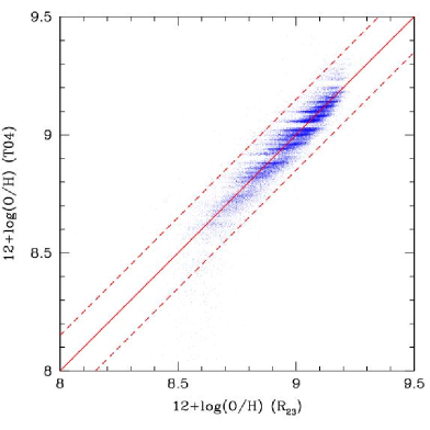
Tremonti et al. (2004) used the approach outlined by Charlot et al. (2006), which consists of estimating metallicities statistically, based on simultaneous fits of all the most prominent emission lines ([O ii], H$\beta$, [O iii], He i, [O i], H$\alpha$, [N ii], [S ii]) with a model designed for the interpretation of integrated galaxy spectra. Here, we use the corresponding emission-line fluxes to directly get dust extinction-corrected $R_{23}$ values first, and then adopt the calibration given by Tremonti et al. (2004) (their eq.1: $12+\mathrm{log(O/H)}=9.185-0.313x-0.264x^{2}-0.321x^{3}$, with $x=\mathrm{log}R_{23}$) to estimate the 12+log(O/H) abundances for our sample galaxies, which we denote as 12+log(O/H)${}_{R_{23}}$. This calibration is only appropriate to the metal-rich branch. The consistency of these two estimates is shown in Fig. 1. The solid line is the line of equality, and the two dashed lines are $\pm$0.15 dex discrepancies from the line of equality. We notice that, for about 260 data points with $12+\mathrm{log(O/H)}<8.5$ estimated by Tremonti et al. (2004), our $R_{23}$-derived abundances are higher than those of Tremonti. All of these galaxies have -1.2$<$[N ii]/H$\alpha$$<$-0.8 (see Fig. 3a), which implies that they are metal poor galaxies on the lower $R_{23}$ branch. Because the calibration of Tremonti et al. is only suitable for the upper branch, we select the galaxies having 8.4$<$12+log(O/H)$<$10 (39,006 objects). We also require the two metallicity estimates to be consistent to $\pm$0.15 dex, which leaves a final sample of 38,478 galaxies.

If a histogram distribution of the 12+log(O/H)${}_{R_{23}}$ is presented, it will show a range of 8.4$<$$12+\mathrm{log(O/H)}$ $<$9.3 with a peak around 12+log(O/H)=9.0 and an increasing gradient-like distribution following the increasing abundance from 8.4 to 9.1. Among these selection criteria, only the 0.04 lower limit of redshift, the 8.4$<$12+log(O/H)$<$10 and the 0.15 dex discrepancy were not considered by Tremonti et al. (2004), others are the same.

3. Deriving calibrations for oxygen abundances from the observations of the SDSS galaxies

We derive the analytic linear least squares and/or third-order polynomial fits from the observed relations of 12+log(O/H)${}_{R_{23}}$ versus “strong-line” ratios of the SDSS sample galaxies: [N ii]/H$\alpha$, [O iii]/[N ii], [N ii]/[O ii], [N ii]/[S ii], [S ii]/H$\alpha$, and [O iii]/H$\beta$. To minimize the systematic uncertainty from calibrations of $R_{23}$ to O/H, we re-derive these calibrations by using two other sets of oxygen abundance estimates replacing 12+log(O/H)${}_{R_{23}}$: 12+log(O/H)_K99, the $R_{23}$-derived abundances by using the $R_{23}$-O/H calibration of Kobulnicky et al. (1999, from McGaugh 1991), and 12+log(O/H)_T04, the Bayesian abundances given by Tremonti et al. (2004). All the calibration coefficients and the rms derivations have been given in Table 1. 12+log(O/H)_K99 is a bit lower than the other two, less than $\sim$0.1 dex lower. In this paper, we only plot the calibration results of 12+log(O/H)${}_{R_{23}}$ versus line ratios as representatives.

The derived calibrations in this paper are only appropriate for the metal-rich galaxies (12+log(O/H)$>$8.4), because the metallicities of these SDSS sample galaxies are in the range of 8.4$<$12+log(O/H)$<$9.3. The corresponding ranges of the various related strong-line ratios will be given in consequent subsections and Table 1. We omit the galaxies with lower metallicities, 12+log(O/H)$<$8.4, in calibrations, and leave them to future work.

3.1. Aperture effects in the SDSS

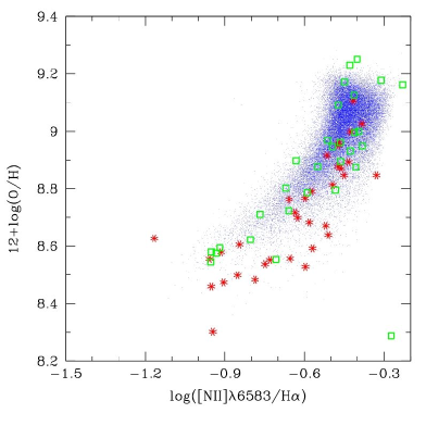
Aperture bias is clearly important when comparing metallicities measured in the central regions of galaxies to “global” quantities such as the luminosity (Kewley et al. 2005). The main question here is if the relation between the metallicity and the ionization parameter is the same in nuclear and global spectra. To estimate the aperture effect on the metallicity estimates, we compare our results about the SDSS galaxies with those of the local Nearby Field Galaxy Survey (NFGS) galaxies from Jansen et al. (2000a,b). Jansen et al. (2000b) have published the emission-line fluxes from both the integrated and nuclear spectra of their galaxies. We calculated their 12+log(O/H) vs. [N ii]/H$\alpha$ relations from their integrated and nuclear spectra, respectively, by using the same method as we adopted for the SDSS galaxies.

We select 38 galaxies from the sample of Jansen et al. (2000b) following the criteria: 1) having the related fluxes for both the integrated and nuclear spectra available; 2) confirming that they are star-forming galaxies by adopting the same criterion of Kauffman et al. (2003b) as we used for the SDSS galaxies; 3) using the same calculation method as for the SDSS galaxies, for example, for estimating $A_{V}$ and deriving (O/H) abundances etc. Fig. 2 shows the comparison with the NFGS galaxies from the integrated spectra (the stars) and the nuclear spectra (the open squares). It is clear that all the data points from the nuclear spectra follow the SDSS galaxies very well, but some data points from the integrated spectra show lower 12+log(O/H) at a given [N ii]/H$\alpha$ value, $\sim$0.1-0.2 dex lower. Fig. 2 may suggest a relatively lower ionization parameter for the outskirt regions of galaxies, but this conclusion is limited by the small number of galaxies with integrated spectra. Therefore, these calibrations from SDSS galaxies may be more suitable to the nuclear spectra of galaxies.

3.2. 12+log(O/H) versus [N ii]/H$\alpha$

The [N ii]/H$\alpha$ ratio is sometimes used to estimate metallicities of galaxies since it is not affected very much by dust extinction due to their close wavelength positions (see Pettini & Pagel 2004). The near infrared spectroscopic instruments, which were developed, can gather these two lines from the galaxies with intermediate and high redshifts.

Metallicity calibrations of log([N ii]$\lambda$6583/H$\alpha$) (the N2 index) can be found in Storchi-Bergmann, Calzetti, & Kinney (1994) and Raimann et al. (2000). Recently, Denicoló et al. (2002) presented an analytical linear formula by fitting the relation of a combined sample of 108 metal-poor galaxies (their O/H abundances were estimated from $T_{e}$) and 128 metal-rich galaxies (their O/H abundances were estimated from $R_{23}$ or $S_{23}$ (= ([S ii]6717,6731+[S iii]9069,9531)/H$\beta$): $12+\log\mathrm{(O/H)}=9.12+0.73\times N2$. The data of Pérez-Montero & Díaz (2005) are generally consistent with this calibration. Pettini & Pagel (2004) obtained a similar linear fit for a sample of 137 galaxies. Most of their samples have 7.0$<$ 12+log(O/H)$<$8.6 based on $T_{e}$ measurements, and six (four are metal-rich) have oxygen abundances obtained from a detailed photoionization model. The linear fit given by Pettini & Pagel (2004) is: $12+\log\mathrm{(O/H)}=8.90+0.57\times N2,$ and another third-order polynomial fit with slight revision is: $12+\log\mathrm{(O/H)}=9.37+2.03\times N2+1.26\times N2^{2}+0.32\times N2^{3}$ (valid in the range of $-2.5<N2<-0.3$).

Here we present the relation of N2 index to (O/H)${}_{R_{23}}$ for the 38,478 SDSS star-forming galaxies, and derive a corresponding calibration from these metal-rich galaxies. Fig. 3a shows our results for 12+log(O/H)${}_{R_{23}}$ vs. N2 index relations (the small blue points, without reddening-correction for [N ii]/H$\alpha$ ratios). The large red squares represent the 29 median N2 values in bins of 0.025 dex in 12+log(O/H) within the range of 12+log(O/H)=8.5 to 9.3. The 12+log(O/H) shows a clear increasing trend following the increase of the N2 index, up to 12+log(O/H)$\sim$ 9.0, and then, the galaxies having 12+log(O/H)$>$ 9.0 show a slightly decreasing N2 index. This trend can be understood as follows: when the secondary production of nitrogen dominates, at somewhat higher metallicity, the [N ii]/H$\alpha$ line ratio continues to increase, despite the decreasing electron temperature; eventually, at still higher metallicities, nitrogen becomes the dominant coolant in the nebula, and the electron temperature falls sufficiently to ensure that the nitrogen line weakens with increasing metallicity (KD02). This is the first large sample to show this turnover relation between N2 and 12+log(O/H) at the very metal-rich region. An analytical third-order polynomial fit to the median-value points can be given in Fig. 3a as the solid line:

$$12+\mathrm{log(O/H)} = a0+a1\times N2+a2\times N2^{2}$$ (3)

$$+ a3\times N2^{3}.$$

The fitting coefficients a0, a1, a2 and a3 are given in Table 1, as well the rms derivation ($\sigma$=0.058 dex) for the data points from the fitting relation. This fit is obtained from the data points with $-1.2<N2<-0.2$ and 8.4$<$ 12+log(O/H)$<$9.3. The two dashed lines describe the discrepancy of 2$\sigma$. A linear fit does not work well for these relations.

However, we should notice that this calibration could result in large uncertainty when 12+log(O/H)$>$9.0 because of the turnover of N2 index versus O/H in the very metal-rich region. Thus, we re-derive a third-order polynomial fit for this calibration for the part of sample galaxies having 8.4$<$12+log(O/H)$<$9.0. We also re-derive the calibrations of the N2 index to 12+log(O/H)_K99 (the dot-long-dashed line in magenta color in Fig. 3a) and 12+log(O/H)_T04. All the fitting coefficients and the rms derivation $\sigma$ values are given in Table 1.

In Fig. 3a we compare our calibration of [N ii]/H$\alpha$ vs. 12+log(O/H) with other two calibrations published recently, as shown by the long-dashed and the dotted lines in Fig. 3a. The long-dashed line represents the linear least squares fit given by Denicoló et al. (2002) for the whole sample of their 236 galaxies. The dotted line refers to the linear least squares fit obtained by Pettini & Pagel (2004) from their 137 sample galaxies. Both of these two calibrations show relatively lower O/H abundance compared to ours at a given N2 index, especially at the very metal-rich part.

The difference from Pettini & Pagel (2004) is easily understood since they only select metal-poor galaxies with $T_{e}$ measurements, except four metal-rich and two metal-poor ones. The fit for these metal-poor galaxies can be directly extrapolated to the metal-rich region and results in a lower O/H at a given [N ii]/H$\alpha$ value there. This may be related to the suggestion of Kennicutt et al. (2003), who pointed out that the abundance estimates from $T_{e}$ method are systematically lower by 0.2-0.5 dex than those derived from the strong-line “empirical” abundance indicators, when the latter are calibrated with theoretical photoionization models.

Denicoló et al. (2002) analyzed their metal-poor and metal-rich galaxies together and used the calibration of Kobulnicky et al. (1999) for converting $R_{23}$ to O/H for most of the metal-rich galaxies. Their fig.1 shows that most of the metal-rich samples indeed lie on the left-top side of the fitting line. If only their metal-rich galaxies were considered to derive a calibration, it will predict a higher oxygen abundance at a given [N ii]/H$\alpha$ ratio than that they derived from the combined sample. To be clear, we re-derive the [N ii]/H$\alpha$ and 12+log(O/H) values for their metal-rich sample galaxies taken from Terlevich et al. (1991), in which the fluxes of the related lines were given as a table. The open triangles in Fig. 3a present the H  ii galaxies from Terlevich et al. (1991) by using the same calibration as ours for the SDSS galaxies. The two samples show consistency. And the data of Terlevich et al. (1991) show more scatter, perhaps it comes from the different slit widths and resolutions used in different runs with different telescopes.

3.3. 12+log(O/H) versus [O iii]/[N ii]

Alloin et al. (1979) firstly introduced the quantity $O3N2=\log${([O iii] $\lambda 5007$/H$\beta$)$/$([N ii] $\lambda 6583$/H$\alpha$)}. Recently, Pettini & Pagel (2004) presented one such calibration by doing linear least squares fitting for a sample of 65 (from the 137) galaxies in the range of $-1<O3N2<1.9$. They obtained a calibration of $12+\log\mathrm{(O/H)}=8.73-0.32\times O3N2.$

We can obtain such a calibration from the large sample of SDSS galaxies. Fig. 3b shows the $R_{23}$-derived 12+log(O/H) versus O3N2 relations for our sample galaxies. The solid line gives a linear least squares fit:

$$12+\log\mathrm{(O/H)}=b0+b1\times O3N2,$$ (4)

with the coefficients b0 and b1 given in Table 1, as well as the rms derivation. The two dashed lines show the discrepancy of 2$\sigma$. The dotted line refers to the fit of Pettini & Pagel (2004) for their 65 metal-poor galaxies, which gives lower O/H than that of our samples at a given O3N2 value; about 0.1 dex lower. The reason may be that the galaxies with $T_{e}$-abundances were mainly used in their study.

To get a better fit for the details of the relation, a third-order polynomial fit is obtained and shown as the long-dashed line in Fig. 3b, which revises the linear equation slightly. The corresponding fitting coefficients of a0, a1, a2 and a3 are given in Table 1 with the same meaning as Eq.(1), as well as the rms derivation. These linear and three-order polynomical calibrations were obtained from the sample galaxies with 8.4$<$ 12+log(O/H) $<$9.3 and -0.7 $<$O3N2$<$ 1.6. The obvious advantages of using the [N ii] and [O iii] lines is that they are unaffected by absorption lines originating from the underlying stellar populations, they lie close to Balmer lines that can be used to eliminate errors due to dust reddening, and they both are strong and easily observable in the optical band.

3.4. 12+log(O/H) versus [N ii]/[O ii]

We can derive the calibration of [N ii]/[O ii] ratio to 12+log(O/H) from the large sample of the SDSS galaxies. Fig. 3c presents these data points in the relation of 12+log(O/H) versus [N ii]/[O ii]. A linear least squares fit reproduces the data distribution well, as shown by the solid line. The two dashed lines show 2$\sigma$ discrepancies. A third-order polynomial fit will revise the fitting equation slightly. The coefficients of the two fits and the rms derivation $\sigma$ of the data to the line are given in Table 1, as well as the appropriate ranges of 12+log(O/H) and log([N ii]/[O ii]). The fitting formulas follow the same format as Eq.(2) and Eq.(1).

Fig. 3c shows that the [N ii]/[O ii] ratios obviously increase with the increasing metallicities, which can be explained by the predominant secondary enrichment of [N ii] above metallicities of 12+log(O/H)$>$8.6 (Alloin et al. 1979; KD02), and the stronger decrease in the number of collisional excitations of the blue [O ii] lines relative to the lower energy [N ii] lines due to the low electron temperature in high metallicity environments.

3.5. 12+log(O/H) versus [N ii]/[S ii]

We can derive the calibration of [N ii]6583/[S ii]6717, 6731 to 12+log(O/H) by using the large sample of SDSS galaxies. Fig. 3d shows these observed results, which can be explained by a linear least squares fit and is given as the solid line. The two dashed lines show the 2$\sigma$ discrepancy. To get a more detailed fit, a third-order polynomial fit has been obtained (the long-dashed line in Fig. 3d), which revises the relation slightly. The coefficients of the two fits and the rms derivations are given in Table 1, as well the appropriate ranges of 12+log(O/H) and log([N ii]/[S ii]). The fitting formulas follow the same format as Eq.(2) and Eq.(1).

It shows that the 12 + log(O/H) abundances of the sample galaxies increase with their log([N ii]/[S ii]) ratios. The reason may be that at high metallicity, nitrogen is a secondary nucleosynthesis element and sulphur is a primary process element (KD02). Both lines have similar excitation potential since they are close to each other in wavelength.

3.6. 12+log(O/H) versus [S ii]/H$\alpha$

Although [S ii]/H$\alpha$ ratio can be easily derived from [N  ii]/H$\alpha$ and [N ii]/[S ii] ratios, it is still interesting to directly present the [S ii]/H$\alpha$ to 12+log(O/H) relations for this large sample of SDSS galaxies. Fig. 3e shows that these data points show a double-valued distribution: because of the turnover around 12+log(O/H)$\sim$8.9-9.0, there will be double-valued oxygen abundances at a given [S ii]/H$\alpha$ ratio. Thus, it is difficult to fit a simple and useful analytic formula from these observational data.

We should notice that the [S ii]/H$\alpha$ ratio has never been suggested or used as a metallicity indicator, because it is far more sensitive to ionization (see Sect.4) than to metallicity, and it results in double-valued (O/H). If it is able to measure the [S ii] and H$\alpha$ lines, it is likely that we have also obtained [N ii], and then we could use the [N ii]/H$\alpha$ calibration.

3.7. 12+log(O/H) versus [O iii]/H$\beta$

The [O iii]4959,5007/H$\beta$ ratios can also be used to estimate the metallicities of galaxies. This was called “$R_{3}$ method” (Edmunds & Pagel 1984), and was shown as: $R_{3}=1.35\times(I_{[OIII]5007}/H\beta),$ and then, $\mathrm{log(O/H)}=-0.69\times\mathrm{log}R_{3}-3.24,$ with a range of -0.6 $\leq$ log$R_{3}$ $\leq$ 1.0 (Vacca & Conti 1992).

Here we present a new calibration for this ratio vs. O/H derived from the SDSS sample galaxies (Fig. 3f). The linear least squares and the third-order polynomial fits are obtained, and given as the solid and the long-dashed lines in Fig. 3f, respectively. The coefficients of the two fits and the rms derivations are given in Table 1 following Eq.(2) and Eq.(1), as well the appropriate ranges of 12+log(O/H) and log$R_{3}$. The two dashed lines show the 2$\sigma$ discrepancy.

The observated results of this large sample of SDSS star-forming galaxies and the derived analytic calibrations show that the higher [N ii]/H$\alpha$, [N ii]/[O ii] and [N ii]/[S ii], and the lower [O iii]/H$\beta$, ([O iii]/H$\beta$)/([N ii]/H$\alpha$) ratios will result in the higher 12+log(O/H) abundances generally. The rms derivations of the observational data relative to the calibration relations are in 0.032-0.078 dex. [N ii]/[O ii] has the lowest rms derivation. These calibrations from strong-line ratios to metallicities can be used to calibrate oxygen abundances of galaxies in future studies.

4. Comparison with the photoionization models

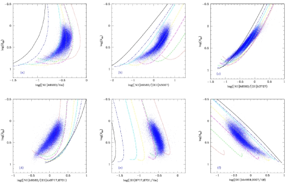
Our strong-line calibrations are in good qualitative agreement with those of KD02. For example, both calibrations show a turnover of [N ii]/H$\alpha$ near 12+log(O/H)$\sim$9.0. One major difference is that KD02 provided strong-line calibrations for seven different values of the ionization parameter, whereas we assume no explicit ionization parameter dependence. Our approach will be less accurate in some cases, but it is necessary when only a few emission lines can be measured and there is too little information to determine both ionization parameter and metallicity. It is also unclear that the full range of ionization parameters used in the KD02 models are required by the data. We explore this in Fig. 4, where we plot the relations between $R_{23}$ and other strong line ratios in the SDSS data and overlay the KD02 model grids. Fig. 5 also gives the similar information.

In Figs. 4a-f, the y-axis log($R_{23}$) is plotted from the lower to the higher values, which corresponds to an increasing trend of metallicity for the galaxies in the metal-rich branch. The seven lines in each plot represent the model results of KD02 for ionization parameters $q=5\times 10^{6}$, $1\times 10^{7}$, $2\times 10^{7}$, $4\times 10^{7}$, $8\times 10^{7}$, $1.5\times 10^{8}$, and $3\times 10^{8}$ cm s^-1, respectively. From the dotted line to the solid line, the ionization parameters increase orderly. The lines in Figs. 4a-f start from 12+log(O/H)=8.4 for the metal-rich branch, and the turn-over trend of the model grids at the low-metallicity end corresponds to the turnover of log($R_{23}$) itself from the metal-rich to the metal-poor branches.

— [N ii]/H$\alpha$     Fig. 4a shows the comparison for log($R_{23}$) versus log([N ii]/H$\alpha$). It shows that these observed points are reasonably consistent with the model results of KD02. The increasing trend of [N ii]/H$\alpha$ follow the decreasing log($R_{23}$)and then the turnover from about log($R_{23}$)$\sim$ 0.5 correspond to the increasing and then the turnover of [N ii]/H$\alpha$ following the increasing 12+log(O/H) abundances as shown in Fig. 3a. However, [N ii]/H$\alpha$ is sensitive to the ionization parameter. It seems that $q=1.5\times 10^{8}$ and $3\times 10^{8}$ cm s^-1 are too high and $q=5\times 10^{6}$ cm s^-1 is too low to explain the distribution of these star-forming galaxies. Most of the sample galaxies fall in the range of ionization parameter $q$ from $1\times 10^{7}$ to $8\times 10^{7}$ cm s^-1, which is narrower than the range proposed by the models.

— [N ii]/[O iii]     Fig. 4b shows the comparison between the observed relations of log($R_{23}$) versus log([N ii]/[O iii]) with the photoionization model results of KD02. It shows that the observed relations are consistent with the model results: the log([N ii]/[O iii]) ratios of these galaxies increase following the decreasing log($R_{23}$) (the increasing metallicities). It also shows that, most of the data points distribute in a range of ionization parameter $q$ from $q=1\times 10^{7}$ to $8\times 10^{7}$ cm s^-1, which is similar to log([N ii]/H$\alpha$). [N ii]/[O iii] is sensitive to the ionization parameter.

—[N ii]/[O ii]     Fig. 4c shows the comparison between the observed results and the photoionization model results of KD02 for the relations of log($R_{23}$) versus log([N ii]/[O ii]). It shows that the [N ii]/[O ii] ratios of the sample galaxies increase following the decreasing log($R_{23}$) (the increasing metallicities), which is very consistent with the general trend of the model results. As KD02 mentioned, [N ii]/[O ii] is almost independent of the ionization parameter. Our large set of data points shows a very narrow distribution in the log($R_{23}$) vs. [N ii]/[O ii] relation, which is very consistent with KD02’s model results. However, [N ii]/[O ii] ratios are affected strongly by dust extinction inside the galaxies. We will discuss this in Fig. 8 and in the last paragraph of this section.

— [N ii]/[S ii]     Fig. 4d shows the comparison between the observed results and the photoionization model results of KD02 for the relations of log($R_{23}$) versus log([N ii]/[S ii]). It shows that the [N ii]/[S ii] ratios of the sample galaxies increase with the decreasing log($R_{23}$) (the increasing metallicities), which is consistent with the general trend of the models. However, the fact is that these SDSS data points show relatively lower log($R_{23}$) (higher metallicities) than the model predicts at a given [N ii]/[S ii] ratio, about 0.2 dex discrepancy. One of the reasons may be that the amount of S going into [S iii] compared to [S ii] is not well understood, so this could introduce some uncertainties into the photoionization models (see KD02). KD02 commented that their [N ii]/[S ii] technique will systematically underestimate the abundance by $\sim$0.2 dex compared to the average of the comparison techniques. The comparison of models and data shows that the models fail to reproduce the strengths of the [S ii] lines, so we cannot use the models to infer abundances or ionization parameters from [N ii]/[S ii], as well [S ii]/H$\alpha$ (see below). These highlight the need for empirical calibration.

— [S ii]/H$\alpha$     Fig. 4e shows the comparison between the observed results and the photoionization model results of KD02 for the relations of log($R_{23}$) versus log([S ii]/H$\alpha$). There is a weak correlation between these two parameters, meaning that log([S ii]/H$\alpha$) decreases following the decreasing log($R_{23}$) with a very weak turnover around log($R_{23}$)$\sim$0.5. For the [S ii]/H$\alpha$ calibration, the SDSS data points agree with a relatively higher model $q$ value than in the [N ii]/[S ii] case.

— [O iii]/H$\beta$     Fig. 4f shows the comparison between the observed results and the photoionization model results of KD02 for the relations of log($R_{23}$) versus log([O iii]/H$\beta$). The model results of [O iii]/H$\beta$ from KD02 were deduced using their three other ratio parameters, i.e. log([N ii]/[O iii]), log([N ii]/[O ii]) and log($R_{23}$), since KD02 did not give a direct formula for this calibration. These SDSS sample galaxies follow the trend of the model results well, meaning the log([O iii]4959,5007/H$\beta$) ratios decrease following the decreasing log($R_{23}$) (the increasing metallicities). This ratio depends strongly on the ionization parameter. Most of the data points are in a range of $q=1\times 10^{7}$ cm s^-1 to $8\times 10^{7}$ cm s^-1, except in the very metal-rich region with log($R_{23}$)$<$0.2.

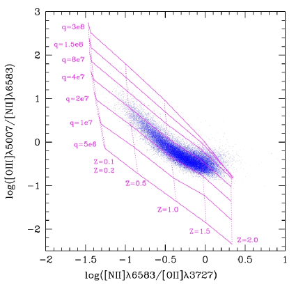
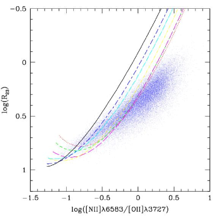
Figs. 4a,b,f show that these star-forming galaxies have a relatively narrower range of ionization parameter $q$ than the range proposed by the photoionization models of KD02. The actual range of $q$ of these galaxies is $1\times 10^{7}$$-$$8\times 10^{7}$ cm s^-1, narrower than the range of models, $q=5\times 10^{6}$$-$$3\times 10^{8}$ cm s^-1. We do not consider Figs. 4c,d,e for this range since [N ii]/[O ii] is insensitive to $q$ and the models provide a poor match to [N ii]/[S ii] and [N ii]/H$\alpha$ (KD02). To show more clearly the range of $q$ of these sample galaxies, we compare their observed results with the model grids in Fig. 5 for the [O iii]/[N ii] versus [N ii]/[O ii] relations following Dopita et al. (2000) (their fig.7). The model grids are taken from Kewley et al. (2001), their instantaneous zero-age starburst models based on the PEGASE spectral energy distribution (SED), which are the most appropriate to use to model H ii regions (KD02), and show information about both metallicity and $q$. This diagram shows that these nearby star-forming galaxies have metallicities $Z=0.2-2.0Z_{\odot}$, and the actual ionization level of their ionized gas have ionization parameters in the range of $q=1\times 10^{7}$ to $8\times 10^{7}$cm s^-1 with some exceptions at the very metal-rich end.

Indeed, the parameter $q$ is related to the ionization parameter $U$ by dividing the speed of light $c$: $U=q/c$, which is more commonly used (e.g. McGaugh 1991). Therefore, the ionization parameters of KD02’s models correspond to a range from log$U$=$-$3.78 to log$U$=$-$2. Our Figs. 4a,b,f show that the actual range of ionization parameters of these SDSS sample galaxies are from about log$U$=$-$3.5 to $-$2.5. This range is also consistent with what found by Dopita et al. (2000) for the extragalactic H ii regions.

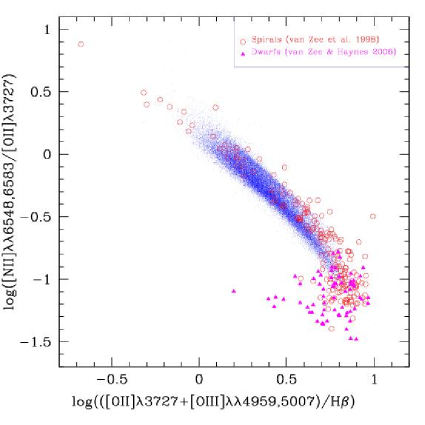
We also compare these SDSS star-forming galaxies with the dwarfs from van Zee & Haynes (2006, the filled triangles) and local spirals from van Zee et al. (1998, the open circles) in Fig. 6 on the basis of the relation of [N ii]/[O ii] versus log$R_{23}$. Although [N ii]/[O ii] is insensitive to ionization parameters, log$R_{23}$ is, so this plot can help to understand the evolutionary status of these sample galaxies. It is clear that these SDSS galaxies follow the metal-rich spirals well, but the dwarfs probe a metallicity range not covered by the SDSS galaxies$-$ only very few dwarfs have 12+log(O/H)$>$8.4.

We should notice that dust extinction will seriously affect the metallicity calibration from the line ratio of [N ii]/[O ii] since the blue line [O ii] is strongly affected by dust extinction. Fig. 7 shows the results without extinction correction for [N ii]/[O ii] for our sample galaxies, which shows a much wider distribution, and is quite far moved from KD02’s model results. The comparison between Fig. 7 and Fig. 4c shows that: 1) the dust extinction in these SDSS galaxies could not be omitted; 2) the extinction coefficients of the individual galaxies are quite different, thus, the data can show large scatter when the dust extinction inside the individual galaxies were not estimated properly. For other ratios, like ([O iii]/H$\beta$)/([N ii]/H$\alpha$), [N ii]/H$\alpha$, [N ii]/[S ii] and[O iii]/H$\beta$, dust extinction does not have much effect on them due to the close positions of the two related lines in wavelength. We did not consider the dust extinction for [N ii]/H$\alpha$ and [N ii]/[S ii ] ratios in our calculations.

5. Nitrogen-to-oxygen abundance ratios

It is possible to estimate the N abundances of galaxies from strong optical emission lines, which can help to understand the origin of nitrogen.

The basic nuclear mechanism to produce nitrogen is well understood – it must result from CNO processing of oxygen and carbon in hydrogen burning. However, the nucleosynthetic origin of nitrogen has a “primary” and a “secondary” component, which is still in debate. If the “seed” oxygen and carbon are those incorporated into a star at its formation and a constant mass fraction is processed, then the amount of nitrogen produced is proportional to the initial heavy-element abundance, and the nitrogen synthesis is said to be “secondary”. If the oxygen and carbon are produced in the star prior to the CNO cycling (e.g. by helium burning in a core, followed by CNO cycling of this material mixed into a hydrogen-burning shell), then the amount of nitrogen produced may be fairly independent of the initial heavy-element abundance of the star, and the synthesis is said to be “primary” (Vila-Costas & Edmunds 1993). In general, primary nitrogen production is independent of metallicity, while secondary production is a linear function of it.

From a theoretical point of view, the $secondary$ production of nitrogen should be common to stars of all masses, whereas the $primary$ production should arise only from intermediate-mass stars ($4<M/M_{\odot}<8$) undergoing dredge-up episodes during the asymptotic giant branch evolution. In particular, when the third dredge-up is operating in conjunction with the burning at the base of a convective envelope (hot-bottom burning), primary nitrogen can originate (Renzini & Voli 1981; Matteucci 1986). The large set of database of galaxies from SDSS must provide important information on the nucleosynthetic origin of nitrogen. The N/O ratio as a function of O/H is the basic method to study the N abundance of galaxies.

5.1. The method and results

Firstly, we use the formula given by Thurston et al. (1996) to estimate the electron temperature in the [N ii] emission region ($T_{[\mathrm{NII]}}$) from log$R_{23}$:

$$T_{[NII]}=6065+1600x+1878x^{2}+2803x^{3},$$ (5)

where $x$=log(R₂₃), $T_{[\mathrm{NII]}}$ is in units of K. This formula was derived from the data points with about -0.6$<$log$R_{23}$$<$0.8, and 5000K$<$$T_{[\mathrm{NII]}}$$<$10000K (see fig.1 of Thurston et al. 1996).

Then, log(N/O) values are estimated from the ([N ii] $\lambda\lambda{6548},{6583}$)/([O ii]$\lambda{3727}$) emission-line ratio and $T_{[\mathrm{NII]}}$ temperature by assuming $\frac{\mathrm{N}}{\mathrm{O}}=\frac{\mathrm{N^{+}}}{\mathrm{O^{+}}}$, and using the convenient formula based upon a five-level atom calculation given by Pagel et al. (1992) and Thurston et al. (1996):

$$\mathrm{log({\frac{{N^{+}}}{{O^{+}}}})} =\mathrm{log{\frac{{[NII]6548,6583}}{{[OII]3727}}}+0.307-0.02log}t_{[NII]}$$ (6)

$$-\frac{{0.726}}{{t_{[NII]}}},$$

where $t_{[NII]}$ = 10^-4$T_{[\mathrm{NII]}}$. We consider the flux of [N ii]$\lambda{6548}$ is equal to one-third (0.333) of that of the [N ii]$\lambda{6583}$ in calculations.

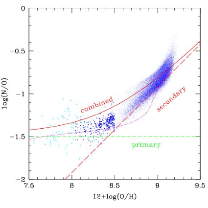
Fig. 8 gives the log(N/O) vs. 12+log(O/H) relations for our sample galaxies. We also plot models for the primary and secondary origin of nitrogen taken from Vila-Costas & Edmunds (1993): the dot-dashed line refers to the “primary” component, the long-dashed line refers to the “secondary” component, and the solid line refers to the combination of the two components. The log(N/O) abundances of the sample galaxies are consistent with the combination of the “primary” and “secondary” components, but the $secondary$ one dominates in these metal-rich galaxies. This result is similar to the previous studies, e.g. Shields et al. (1991), Vila-Costas & Edmunds (1993), Contini et al. (2002), and Kennicutt et al. (2003). In addition, 67 H ii regions in 21 dwarf irregular galaxies taken from van Zee & Haynes (2006) are also plotted in Fig. 8 as triangles. The log(N/O) abundances of these dwarf irregulars are dominated by the “primary” component. The SDSS galaxies with 8.0$<$12+log(O/H)$<$8.5 in the metallicity transition region are also presented as the $stars$ in Fig. 8. They are just distributed in the region between the H ii regions in dwarf irregulars and the metal-rich galaxies.

5.2. The analyses and discussions

The SDSS sample galaxies show increasing log(N/O) abundance ratios following increasing 12+log(O/H) abundances. The behavior of N/O with increasing metallicity provides clues about the chemical evolution history of the galaxies and the stellar populations responsible for producing oxygen and nitrogen. Oxygen is mainly produced in short-lived, massive stars, and is ejected to the ISM by Type II supernova explosions (SNe). In addition, nitrogen is mainly produced in the long-lived, intermediate- and low-mass stars, and is ejected to ISM through stellar wind. In particular, the burning at the base of the convective envelope (hot-bottom burning) and in conjunction with the third dredge-up process in intermediate-mass stars contribute an important fraction of nitrogen (Renzini & Voli 1981; van den Hoek & Groenewegen 1997; Liang et al. 2001; Henry et al. 2000). Therefore, nitrogen will be delayed in its release into the ISM as compared to oxygen.

Contini et al. (2002) analyzed the delayed release of nitrogen. As they discussed, during a long period of quiescence, intermediate-mass star evolution will significantly enrich the galaxy in nitrogen but not in oxygen; during starburst, however, N/O drops while O/H increases as the most massive stars begin to die and supernovae release oxygen into the ISM. A few tens of Myr after the burst, the massive stars producing oxygen will be gone. Then N/O will rise again as intermediate-mass stars begin to contribute to the primary and secondary production of nitrogen. A galaxy undergoing successive starbursts will make the N/O ratio increase following the increasing O/H abundance. However, the increasing N/O following O/H in the metal-rich region does not have to require star formation to occur in periodic starbursts. Rather, as long as the recent star formation activity is less than the past star formation rate, the delayed release of nitrogen from the aggregate intermediate mass stellar population will slowly increase the N/O ratio since it is not balanced by additional production of oxygen in high mass stars (van Zee & Haynes 2006).

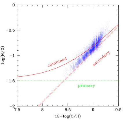
One fact in Fig. 8 should be noticed: when the O/H increases to be 12+log(O/H)$\sim$9.0, the slope of the increase of log(N/O) becomes steeper, i.e. the log(N/O) shows an upturn trend at higher metallicities than 12+log(O/H)$\sim$9.0, or O/H then saturates for the increasing N/O. The main reason for this may be that the sensitivity of $R_{23}$ to metallicity saturates somewhat at a high metallicity. To understand more about this, we rederive the relations of log(N/O) versus the other two sets of $R_{23}$-derived oxygen abundances, 12+log(O/H)_K99 and 12+log(O/H)_Z94. The later one is derived from the conversion of $R_{23}$ to 12+log(O/H) given by Zaritsky et al. (1994). They show the same trend as 12+log(O/H)${}_{R_{23}}$. We then take the Bayesian estimates of 12+log(O/H)_T04 from Tremonti et al. (2004) to replace the $R_{23}$-derived oxygen abundances to present the N/O vs. O/H relations of the sample galaxies. The results are given in Fig. 9. The saturation of 12+log(O/H) to log(N/O) becomes much weaker now. This confirms that the saturation of O/H to N/O at the metal-rich end mainly comes from the insensitivity of $R_{23}$ to 12+log(O/H) there. Indeed, our Fig. 1 has shown this saturation of $R_{23}$-derived oxygen abundances at the high metallicity end. That may mean that the upturn in N/O at high abundance is not physical.

From the comparisons above, we should note that care should be taken in interpreting features in the N/O vs. O/H diagram because of systematic uncertainties in metallicity calibration. If we use $T_{e}$ rather than strong-line calibrations, O/H would be lower but N/O would not be much affected since it has only a weak dependence on $T_{e}$. The net effect would be a shift of the data to the left in Figs. 8,9. The data points will then be more consistent with the H ii regions in M101 studied by Kennicutt et al. (2003) in the relations of N/O vs. O/H diagram. The magenta dotted line in Fig. 8 is the “best” model B of the numerical one-zone models for the evolution of N/O versus O/H given by Henry et al. (2000). Kennicutt et al. (2003) found that the predicted N/O mode by this model is too low at intermediate abundance (12+log(O/H)${}_{T_{e}}$=8.2-8.6) to predict the observed results of the H ii regions in M101. Our SDSS sample galaxies show a similar discrepancy from the model: at the intermediate abundance 12+log(O/H)$<$9.0, the model predicts too low N/O at a given O/H; for the 12+log(O/H)$>$9.0, although the model predicts an increasing trend of N/O following O/H, the predicted N/O is still generally lower than the observed results at a given O/H. Indeed, Henry et al. (2000) themselves already pointed out that their model B provides a fit to the NO envelope compared with the observational data (see their fig.3b).

In addition, dust extinction is a very important factor affecting the estimated (N/O) abundances, as well as the O/H abundances. It can be understood from Fig. 7 (by comparing with Fig. 4c). The dust extinction of these SDSS sample galaxies has been considered when deriving their abundances. Moreover, it is a homogeneous sample taken from one single facility using the same set-up, which minimizes the systematic errors from observation runs, and the [N ii]/[O ii] ratio is almost independent of the ionization parameter (KD02). Therefore, these SDSS data points would not show much spread in the N/O vs O/H relations due to observational errors. The observational scatter of these galaxies are about 0.062 dex estimated from Fig. 9.

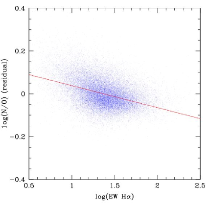
The scatter in the observed log(N/O) vs. log(O/H) relation is relatively small. Nevertheless, we can use our large dataset to see if the residuals correlate with any physical properties of galaxies. If the release of nitrogen is indeed delayed with respect to oxygen, we might expect to find a correlation between the N/O residuals and the stellar birthrate, which is the ratio of the present to past average star formation rate (SFR). The equivalent widths of H$\alpha$ emission lines, log(EW(H$\alpha$)), provides a good proxy for the stellar birthrate (Kennicutt et al. 1994). Fig. 10 shows the relation between log(N/O)_residual and the log(EW(H$\alpha$)) for the sample galaxies. log(N/O)_residual is the N/O abundance having its dependence on O/H abundances been removed. To do so, first we obtain a linear least squares fit for the relation between log(N/O) vs. 12+log(O/H)_T04 for the sample galaxies, then the observed log(N/O) abundances were subtracted by the fitted values predicted by this linear relation. Fig. 10 shows that the log(N/O) abundances decrease following the increasing EWs(H$\alpha$) for these galaxies. The solid line refers to a linear least squares fit for this observed relation with a rms $\sim$0.057:

$$\mathrm{log({\frac{{N}}{{O}}})_{residual}=-0.102\times log(EW(H\alpha))+0.140.}$$ (7)

This relation means that the log(N/O) increases following the decreasing star formation rates, which is consistent with the suggestion of van Zee & Haynes (2006) for the relation between log(N/O) and B-V colors for their dwarf galaxies. They suggested that the high N/O ratio are correlated with redder systems and decreasing star formation rates.

6. Conclusion

We have use the observational data of a large sample of 38,478 star-forming galaxies selected from SDSS-DR2 to derive oxygen abundance calibrations of 12+log(O/H) versus several metallicity-sensitive emission-line ratios, including [N ii]/H$\alpha$, [O iii]/[N ii], [N ii]/[O ii], [N ii]/[S ii], [S ii]/H$\alpha$, and [O iii]/H$\beta$. These calibrations are very useful when the “$T_{e}$-method”, the most accurate method, and the empirical “$R_{23}$-method” are not available to estimate oxygen abundances of galaxies. In addition, they can overcome the “double-valued” drawback of the $R_{23}$-method.

We fit the observed relations with a linear least squares fit and/or a third-order polynomial fit. All the fitting coefficients and the rms derivations (0.032-0.078 dex) have been given in Table 1. When we only select the sample galaxies with higher signal-to-noise ratio emission lines, e.g. $>$10$\sigma$, the rms derivations only have small changes, which means that probably most of the scatter is intrinsic and not an artifact of observational errors. The scattering of the data points mainly come from the different ionization parameters in the individual galaxies, which is confirmed by the smallest rms value of [N ii]/[O ii] ratio, which is independent on the ionization parameters. Such a large sample of galaxies can show some information never before obtained from much smaller samples, for example, the turnover of the relations between 12+log(O/H) versus [N ii]/H$\alpha$ at 12+log(O/H)$>$9.0.

Among these calibrations, the [N ii]/[O ii] ratio should be the best one for metallicity calibration in the metal-rich branch (same as KD02) because it shows a monotonical increase following the increasing metallicity and less scatter than other line ratios, and it is independent of the ionization parameter. However, dust extinction must be estimated properly before using this calibration indicator because of the blue line [O ii] and the far positions of the two lines in wavelength. ([O iii]/H$\beta$)/([N ii]/H$\alpha$) is also a good indicator, a bit better than [N ii]/[S ii] and [O iii]/H$\beta$ due to the relatively smaller rms derivation. The discrepancy between the data and models for [N ii]/[S ii] highlights the need for empirical calibrations. [N ii]/H$\alpha$ is only a good indicator for the galaxies with 12+log(O/H)$<$9.0, and the problem at higher metallicities is the turnover of [N ii]/H$\alpha$ following increasing O/H. However, [N ii]/H$\alpha$ may be one of the most useful calibrations since it is not affected by dust extinction due to the very close positions of the two related lines in wavelength, and can be detected by the near infrared instruments for the intermediate- and high-$z$ star-forming galaxies. We should notice that the derived calibration will result in a higher 12+log(O/H) abundance at a given [N ii]/H$\alpha$ ratio than those of Pettini & Pagel (2004) and Denicoló et al. (2002). The main reason for this difference may be due to the discrepancy between the metallicity estimates from the $T_{e}$-method and $R_{23}$-method.

The resulting calibrations are more suitable for luminous and metal-rich galaxies since they have metallicities in the range 8.4$<$ 12+log(O/H)${}_{R_{23}}$ $<$9.3. Because our calibrations are derived from SDSS data, they will be best suited for data which samples the inner few kiloparsecs of galaxies rather than the whole disk. This aperture effect is most significant for line ratios with a strong dependence on ionization parameter (e.g. [N ii]/[O iii]).

The observed calibration relations are compared with the photoionization models from KD02, which generally show good consistent trends, including the turnover trend of [N ii]/H$\alpha$ at the metal-rich end, the independence of [N ii]/[O ii] on ionization parameter, etc. However, most of these sample galaxies are distributed in a narrower range of the ionization parameter $q$ than the models. The actual range of $q$ is from $1\times 10^{7}$ to $8\times 10^{7}$ cm s^-1, i.e., log$U$=-3.5 to -2.5, but the models cover from $q=5\times 10^{6}$ to $3\times 10^{8}$ cm s^-1, i.e., log$U$=-3.78 to -2.

Another contribution of this work is that we obtained the log(N/O) abundance ratios for this large sample of SDSS star-forming galaxies with 8.4$<$ 12+log(O/H)$<$9.3. Their log(N/O) abundances are consistent with the combination of the “primary” and “secondary” components of nitrogen, but the “secondary” one dominates at high metallicities. The increasing log(N/O) abundances that follow the increasing metallicities for these metal-rich galaxies can be the prediction of continuous but declining star formation rates, which is confirmed by the linear relation with a negative slope of the log(N/O)_residual versus log(EW(H$\alpha$)). The scatter of these observational data are $\sim$0.062 dex in the log(N/O) versus 12+log(O/H) relations. However, we should notice that dust extinction strongly affects the estimates of the log(N/O) abundance ratios and the corresponding scatter for the sample galaxies.

In summary, this work provides several useful metallicity calibrations based on strong emission-line ratios of 38,478 SDSS star-forming galaxies, and estimates the log(N/O) abundance ratios for such a large number of galaxies. These can be used as references for future studies of metallicities of galaxies. We should notice that, when these calibrations are used for high redshift objects, the indices based on [N ii] may have some extra uncertainties since for very high redshifts N/O vs. O/H may be different from the local case because the galaxies are not old enough to produce significant amounts of secondary nitrogen.

Figure 1.— Comparison between our metallicity estimates from the extinction-corrected $R_{23}$ parameters ($R_{23}$) and those Bayesian estimates from Tremonti et al. (2004) (T04) derived using the model of Charlot et al. (2006). These two estimates are very consistent. The solid line refers to the line of equality, and the $\pm$0.15 dex discrepancies from the solid line are also given as the two dashed lines.

Figure 2.— Comparison between our sample galaxies (the small blue points) and the NFGS galaxies at local from Jansen et al. (2000a,b): ${the~{}stars}$ refer to the results from the integrated spectra, and ${the~{}open~{}squares}$ refer to the results from the nuclear spectra (see text).

Figure 3.— Analytic calibration relations between 12+log(O/H) and several metallicity-sensitive strong-line ratios based on the observed relations of the SDSS sample galaxies ($the$ $small~{}blue~{}points$): (a.) versus N2 index (without reddening correction for [Nii]/H$\alpha$). The large squares represent the 29 median values in bins of 0.025 dex in 12+log(O/H) within 12+log(O/H) from 8.5 to 9.3. The open triangles refer the local H ii galaxies from Denicoló et al. (2002) (from Terlevich et al. 1991). The dot-long-dashed line represents the calibration with 12+log(O/H)_K99. (b.) versus O3N2 index relations. (c.) versus log([N ii]/[O ii]). (d.) versus log([N ii]/[S ii]) (without reddening correction for [Nii]/[S ii]). (e.) versus log([S ii]/H$\alpha$). (f.) versus log([O iii]/H$\beta$) ratios. The solid lines refer to the fits to the data (see text), and the two dashed-lines show the discrepancy of 2$\sigma$; the long-dashed lines in Figs.b,c,d,f refer to the three-order polynomial fits for the observational relations. The dotted lines in Figs.a,b refer to the linear least-squares fit given by Pettini & Pagel (2004), the long-dashed line in Fig.a refers to the result of Denicoló et al. (2002). The dot-long-dashed line in Fig.f refers to the linear least-squares fit given by Vacca & Conti (1992). All the fitting coefficients for the SDSS galaxies and the rms derivations have been given in Table 1 following the format of Eq.(2) and Eq.(1).

Figure 4.— Comparison between our SDSS sample galaxies ($the$ $small~{}blue~{}points$) and the photoionization model results of KD02 ($the~{}lines$) for the relations of log($R_{23}$) versus several strong-line ratios: (a.) log([N ii]/H$\alpha$); (b.) log([N ii]/[O iii]); (c.) log([N ii]/[O ii]); (d.) log([N ii]/[S ii]); (e.) log([S ii]/H$\alpha$); (f.) log([O iii]/H$\beta$). The lines represent the model results of KD02 with $q=5\times 10^{6}$, $1\times 10^{7}$, $2\times 10^{7}$, $4\times 10^{7}$, $8\times 10^{7}$, $1.5\times 10^{8}$, and $3\times 10^{8}$ cm s^-1, shown as from the red dotted line to the black solid line, respectively. The seven lines in Fig.f were deduced from other three line ratios, i.e. log([N ii]/[O iii]), log([N  ii]/[O ii]) and log($R_{23}$), since there are no direct log([O iii]/H$\beta$) calibration relation given in KD02.

Figure 5.— Comparison between the observed results of the SDSS sample galaxies and the photoionization models of Kewley et al. (2001) following fig.7 of Dopita et al. (2000). The solid lines refer to constant ionization parameters, with the grids of $q=5\times 10^{6}$, $1\times 10^{7}$, $2\times 10^{7}$, $4\times 10^{7}$, $8\times 10^{7}$, $1.5\times 10^{8}$, $3\times 10^{8}$ cm s^-1; and the dotted lines refer to constant metallicity, with the grids of $Z=$0.1, 0.2, 0.5, 1.0, 1.5 and $2.0Z_{\odot}$.

Figure 6.— Comparison between our sample galaxies and the spiral galaxies form van Zee et al. (1998) and the dwarf irregulars from van Zee & Haynes (2006).

Figure 7.— Comparison the log($R_{23}$) versus log([N ii]/[O ii]) relations between our sample galaxies without correcting dust extinction for [N ii]/[O ii] and the model results of KD02. The comparison of this plot with Fig. 4c shows that the dust extinction strongly affect the [N ii]/[O ii] ratios and their scatter, hence the calibrated metallicities.

Figure 8.— log(N/O) abundance ratios of our SDSS sample galaxies as functions of their 12+log(O/H) abundances derived from $R_{23}$ by using the calibration given by Tremonti et al. (2004). $The$ $small~{}blue~{}points$ refer to the observational data on metal-rich branch, and $the$ $stars$ refer to the SDSS sample galaxies with lower metallicities, 12+log(O/H)=8.0-8.5, which are the Bayesian metallicity estimates from Tremonti et al. (2004) and are in the “transition region” from the metal-poor to the metal-rich branches. The $open~{}triangles$ in cyan color represent the 67 H ii regions in 21 dwarf irregular galaxies taken from van Zee & Haynes (2006). The “primary” (the dot-dashed line), “secondary” (the long-dashed line) components and the combination of these two components (the solid line) taken from Vila-Costas & Edmunds (1993) have also been plotted. The dotted line refers to the prediction of a numerical one-zone model from Henry et al. (2000).

Figure 9.— log(N/O) abundance ratios of the SDSS sample galaxies as a function of the Bayesian metallicity estimates 12+log(O/H)_T04 from Tremonti et al. (2004). The lines are the same as in Fig. 8.

Figure 10.— log(N/O) abundance residuals of our SDSS sample galaxies as a function of the equivalent widths of their H$\alpha$ emission lines EWs(H$\alpha$) (in Å). The solid line refers to a linear least-squares fit with a rms $\sim$0.057 for the data points (Eq.(5)).

Table 1Coefficients for the oxygen abundance diagnostics. Defining oh=12+log(O/H) here; assuming y=b0+b1x, and y=a0+a1x+a2x²+a3x³ for the linear and 3-order polynomial fits, respectively. Here, y=log$R_{23}$, 12+log(O/H)${}_{R_{23}}$, 12+log(O/H)_T04 and 12+log(O/H)_K99 for the different cases, and x= N2, O3N2, N2O2, N2S2, O3Hb for each of the “y” case. $\sigma$ is the rms deviation from the data to the fitted line in dex.

(1)	(2)	(3)	(4)	(5)	(6)	(7)
diagnostics	N2	N2	O3N2	N2O2	N2S2	O3Hb
	log${\frac{{[NII]6583}}{{H\alpha}}}$	log${\frac{{[NII]6583}}{{H\alpha}}}$	log${\frac{{[OIII]5007/H\beta}}{{[NII]6583/H\alpha}}}$	log${\frac{{[NII]6583}}{{[OII]3727}}}$	log${\frac{{[NII]6583}}{{[SII]6717,6731}}}$	log${\frac{{[OIII]4959,5007}}{{H\beta}}}$
appropriate range	[-1.2,-0.55]	[-1.2,-0.2]	[-0.7,1.6]	[-1.4,0.7]	[-0.5,0.8]	[-0.9,0.6]
	8.4$<$oh$<$9.0	8.4$<$oh$<$9.3
			Linear fits
12+log(O/H)${}_{R_{23}}$
b0	…	…	9.010	9.125	8.944	8.846
b1	…	…	-0.373	0.490	0.669	-0.497
$\sigma$(dex)	…	…	0.059	0.039	0.075	0.062
12+log(O/H)T04
b0	…	…	9.007	9.128	8.934	8.845
b1	…	…	-0.384	0.514	0.789	-0.490
$\sigma$(dex)	…	…	0.067	0.041	0.050	0.078
12+log(O/H)K99
b0	…	…	8.916	9.020	8.857	8.771
b1	…	…	-0.332	0.443	0.605	-0.441
$\sigma$(dex)	…	…	0.058	0.037	0.068	0.061
			Polynomial fits
12+log(O/H)${}_{R_{23}}$
a0	10.305	11.948	9.013	9.118	8.956	8.841
a1	4.786	11.843	-0.395	0.338	0.746	-0.575
a2	5.079	14.986	-0.072	-0.319	-0.472	0.011
a3	2.191	6.747	0.106	-0.125	-0.807	0.297
$\sigma$(dex)	0.063	0.058	0.058	0.035	0.072	0.061
12+log(O/H)T04
a0	9.617	11.835	9.011	9.121	8.945	8.839
a1	1.563	11.317	-0.406	0.384	0.838	-0.584
a2	0.262	14.289	-0.086	-0.229	-0.380	0.001
a3	-0.048	6.566	0.119	-0.052	-0.481	0.342
$\sigma$(dex)	0.051	0.050	0.066	0.038	0.048	0.076
12+log(O/H)K99
a0	12.074	12.464	8.919	9.014	8.868	8.762
a1	14.410	15.612	-0.358	0.287	0.682	-0.514
a2	21.398	22.305	-0.085	-0.362	-0.423	0.076
a3	11.193	11.185	0.126	-0.171	-0.842	0.368
$\sigma$(dex)	0.070	0.065	0.057	0.032	0.066	0.059

References

- (1) Abazajian, K., Adelman-McCarthy, J. K., Agüeros, M. A. et al. 2004, AJ, 128, 502
- (2) Aller, L.H. 1942, ApJ, 95, 52
- (3) Aller, L.H. 1990, PASP, 102, 1097
- (4) Alloin, D., Collin-Souffrin, S., Joly, M., Vigroux, L., 1979, A&A, 78, 200
- (5) Baldwin, J. A., Phillips, M. M., Terlevich, R., 1981, PASP, 93, 5 (BPT)
- (6) Bresolin, F., Schaerer, D., González Delgado, R. M., Stasińska, G., 2005, A&A, 441, 981
- (7) Bresolin, F., Garnett, D. R., Kennicutt, R. C. Jr., 2004, ApJ, 615, 228
- (8) Brinchmann, J., Charlot, S., White, S. D. M., Tremonti, C., Kauffmann, G., Heckman, T., Brinkmann, J., 2004, MNRAS, 351, 1151
- (9) Charlot, S. et al. 2006 (in preparasion)
- (10) Charlot, S. & Longhetti, M., 2001, MNRAS, 323, 887
- (11) Contini, T., Treyer, M. A., Sullivan, M., Ellis, R. S., 2002, MNRAS, 330, 75
- (12) de Robertis, M. M. ApJ, 1987, 316, 597
- (13) Denicoló, G., Terlevich, R., Terlevich, E., 2002, MNRAS, 330, 69
- (14) Dopita, M. A. & Evans, I. N. 1986, ApJ, 307, 431
- (15) Dopita, M. A., Kewley, L. J., Heisler, C. A., Sutherland, R. S., 2000, ApJ, 542, 224
- (16) Edmunds, M. G., Pagel, B. E. J. 1984, MNRAS, 211, 507
- (17) Garnett, D. R., Kennicutt, R. C. Jr., Bresolin, F., 2004a, ApJ, 607, L21
- (18) Garnett, D. R., Edmunds, M. G., Henry, R. B. C., Pagel, B. E. J., Skillman, E. D., 2004b, AJ, 128, 2772
- (19) Henry, R. B. C., Edmunds, M. G., Köppen, J. 2000, ApJ, 541, 660
- (20) Jansen, R. A., Franx, M., Fabricant, D., Caldwell, N., 2000a, ApJS, 126, 271
- (21) Jansen, R. A., Fabricant, D., Franx, M., Caldwell, N., 2000b, ApJS, 126, 331
- (22) Kauffmann, G., Heckman, T.M., White, S. D. M. et al. 2003a, MNRAS, 341, 33
- (23) Kauffmann, G., Heckman, T. M., Tremonti, C. et al. 2003b, MNRAS, 346, 1055
- (24) Kennicutt, R. C. Jr., Bresolin, F., Garnett, D. R., 2003, ApJ, 591, 801
- (25) Kennicutt, R. C. Jr., Tamblyn, P., Congdon, C. W., 1994, ApJ, 435, 22
- (26) Kewley, L. J. & Dopita, M. A. 2002, ApJS 142, 35 (KD02)
- (27) Kewley, L. J., Dopita, M. A., Sutherland, R. S. et al. 2001, ApJ, 556, 121
- (28) Kewley, L. J., Jansen, R. A., Geller, M. J., 2005, PASP, 117, 227
- (29) Kim, M., Ho, L. C., Im, M., 2006, astro-ph/0601316
- (30) Kobulnicky, H. A., Kennicutt, R. C. Jr. & Pizagno, J. L.,1999, ApJ, 514, 544 (K99)
- (31) Liang, Y. C., Zhao, G., Shi, J. R. 2001, A&A, 374, 936
- (32) Matteucci, F. 1986, MNRAS, 221, 911
- (33) McCall, M. L., Rybski, P. M., Shields, G. A. 1985, ApJS, 57, 1
- (34) McGaugh, S. S. 1991, ApJ, 380, 140
- (35) Osterbrock, D. E. 1989, Astrophysics of Gaseous Nebulae and Active Galactic Nuclei. Mill Valley, California: University Science Books
- (36) Pagel, B.E.J., 1986, PASP, 98, 1009
- (37) Pagel, B. E. J., Edmunds, M. G., Blackwell, D. E. et al. 1979, MNRAS, 189, 95
- (38) Pagel, B. E. J., Edmunds, M. G., Smith, G., 1980, MNRAS, 193, 219
- (39) Pagel, B.E.J., .Simonson, E. A., Terlevich, R. J., Edmunds, M. G. 1992, MNRAS, 255, 325
- (40) Peimbert, M. 1975, ARA&A, 13, 113
- (41) Peimbert, M.,Rayo, J. F. & Torres-Peimbert, S., 1975, RmxAA, 1, 289
- (42) Pérez-Montero, E. & Díaz, A. I., 2005, MNRAS, 361, 1063
- (43) Pettini, M. & Pagel. B. E. J., 2004, MNRAS, 348, L59
- (44) Pilyugin, L. S. 2000, A&A, 362, 325
- (45) Pilyugin, L. S. 2001a, A&A, 369, 594
- (46) Pilyugin, L. S. 2001b, A&A, 373, 56
- (47) Raimann, D., Storchi-Bergmann, T., Bica, E., Melnick, J., Schmitt, H., 2000, MNRAS, 316, 559
- (48) Renzini,A. & Voli,M. 1981, A&A, 94, 175
- (49) Salpeter, E. E. 1955, ApJ, 121, 161
- (50) Salzer, J. J., Lee, J. C., Melbourne, J., Hinz, J. L., Alonso-Herrero, A., Jangren, A., 2005, ApJ, 624, 661
- (51) Searle, L. 1971, ApJ, 168, 327
- (52) Seaton, M. J. 1979, MNRAS 187, 73
- (53) Schlegel, D. J., Finkbeiner, D. P., Davis, M., 1998, ApJ, 500, 525
- (54) Shields, G.A., 1990, ARA&A, 28, 525
- (55) Shields, G. A., Skillman, E. D., Kennicutt, R. C. Jr, 1991, ApJ, 371, 82
- (56) Skillman, E. D. Côté, S., Miller, B. W., 2003, AJ, 125, 610
- (57) Skillman, E. D. & Kennicutt,R.C. Jr. 1993, ApJ, 411, 655
- (58) Skillman,E. D., Kennicutt,R.C. Jr., Hodge, P.W., 1989, ApJ, 347, 875
- (59) Stasińska, G. & Leitherer, C. 1996, ApJS, 107, 661
- (60) Stasińska, G. 2002, lectures to be published in the proceedings of the XIII Canary Islands Winter School of Astrophysics, astro-ph/0207500
- (61) Storchi-Bergmann, T., Calzetti, D., Kinney, A. L., 1994, ApJ, 429, 572
- (62) Strauss, M. A., Weinberg, D. H., Lupton, R. H., 2002, AJ, 124, 1810
- (63) Thurston, T. R., Edmunds, M. G., Henry, R. B. C. 1996, MNRAS, 283, 990
- (64) Torres-Peimbert,S., Peimbert,M. & Fierro,J. 1989, ApJ, 345, 186
- (65) Tremonti, C. A., Heckman, T. M., Kauffmann, G. et al. 2004, ApJ, 613, 898 (T04)
- (66) Vacca, W. D. & Conti, P. S., 1992, ApJ, 401, 543
- (67) van den Hoek, L. B. & Groenewegen, M. A. T. 1997, A&AS, 123, 305
- (68) van Zee, L., Salzer, J. J., Haynes, M. P., 1998, ApJ, 497, L1
- (69) van Zee, L. & Haynes, M. P. 2006, ApJ, 636, 214
- (70) Vila-Costas, M. B. & Edmunds, M. G. 1993, MNRAS, 265, 119
- (71) Veilleux, S. & Osterbrock, D. E., 1987, ApJS, 63, 295
- (72) Zaritsky, D., Kennicutt, R. C., Huchra, J. P., 1994, ApJ, 420, 87 (Z94)