A Structured Leptonic Jet Model of the “Orphan” TeV Gamma-Ray Flares in TeV Blazars

Abstract

The emission spectra of TeV blazars extend up to tens of TeV and the emission mechanism of the TeV $\gamma$-rays is explained by synchrotron self-Compton scattering in leptonic models. In these models the time variabilities of X-rays and TeV $\gamma$-rays are correlated. However, recent observations of 1ES 1959+650 and Mrk 421 have found the “orphan” TeV $\gamma$-ray flares, i.e., TeV $\gamma$-ray flares without simultaneous X-ray flares. In this paper we propose a model for the “orphan” TeV $\gamma$-ray flares, employing an inhomogeneous leptonic jet model. After a primary flare that accompanies flare-up both in X-rays and TeV $\gamma$-rays, radiation propagates in various directions in the comoving frame of the jet. When a dense region in the jet receives the radiation, X-rays are scattered by relativistic electrons/positrons to become TeV $\gamma$-rays. These $\gamma$-ray photons are observed as an “orphan” TeV $\gamma$-ray flare. The observed delay time between the primary and “orphan” flares is about two weeks and this is accounted for in our model for parameters such as $\Gamma=20$, $d=4\times 10^{17}$cm, $\alpha=3$, and $\eta=1$, where $\Gamma$ is the bulk Lorentz factor of the jet, $d$ is the distance between the central black hole and the primary flare site, $\alpha/\Gamma$ is the angle between the jet axis and the direction of the motion of the dense region that scatters incoming X-rays produced by the primary flare, and $\eta/\Gamma$ is the angle between the jet axis and the line of sight.

1 Introduction

Blazars are a subclass of active galactic nuclei and their high energy emission is generated in regions near the central super massive black holes. Because of their intense and rapidly variable radiation, the emission regions are thought to be in relativistic jets closely aligned to the line of sight (see Aharonian, 2004; Krawczynski, 2004, for a review). The spectral energy distributions (SEDs) of blazars are characterized by double broad peaks in the $\nu$-$\nu F_{\nu}$ representation. One peak is in the optical to X-ray regions and the other is in the $\gamma$-ray region. Very high energy (100 MeV – 1 GeV) $\gamma$-rays from blazars were discovered by EGRET (Energetic Gamma-Ray Experiment Telescope) on board Compton Gamma-Ray Observatory (Hartman et al., 1999). Recent observations by Cerenkov telescopes have revealed that many blazars emit $\gamma$-rays up to tens of TeV (Aharonian et al., 2005, for a review). Flare activities in X-rays and $\gamma$-rays from blazars are also known. Although the emission mechanisms of blazars are still under study, the SEDs of blazars are well explained by leptonic or hadronic models. In the framework of the leptonic models, the emission in the optical to X-ray region is attributed to synchrotron radiation by nonthermal electrons/positrons in the jet and the TeV $\gamma$-rays are accounted for by the synchrotron self-Compton (SSC) model (Maraschi et al., 1992). The SSC model assumes that synchrotron photons are inverse-Compton scattered by the same nonthermal electrons/positrons that emit synchrotron photons. If the SSC model is applied, the time variabilities of the X-rays and $\gamma$-rays should be correlated (e.g., Mastichiadis & Kirk, 1997; Li & Kusunose, 2000; Kusunose et al., 2000), and indeed most flares occur almost simultaneously in X-rays and $\gamma$-rays. However, the recent observations of 1ES 1959+650 (Krawczynski et al., 2004; Daniel et al., 2005) found that there is a TeV $\gamma$-ray flare that is not accompanied by a X-ray flare, which was observed on June 4, 2002 (MJD 52,429) by the Whipple telescope. This is called the “orphan” TeV $\gamma$-ray (OTG) flare. The OTG flare occurred about 15 days after a usual flare in which X-ray and $\gamma$-ray flares were observed contemporaneously. More recently another OTG flare might have been observed from Mrk 421 (Błażejowski et al., 2005), although the X-ray flux seems to have peaked about 1.5 days before this TeV flare and this may not be a true OTG flare.

The existence of the OTG flares is challenging for the leptonic models. Böttcher (2005) has recently proposed a model for the OTG flare of ES 1959+650, i.e., the hadronic synchrotron mirror model. He assumed that a fraction of X-rays produced in the primary flare by synchrotron radiation of leptons is reflected by a plasma cloud with scattering depth $\sim 0.1$ located in the direction of the jet propagation. The reflected X-rays collide with protons in the jet and pions are produced. Subsequently a large number of neutral pions decay into $\gamma$-rays, which are expected to be observed as TeV $\gamma$-rays. If this model is applied to 1ES 1959+650, it is found that the reflecting plasma is located at a distance $\sim 3(\Gamma/10)^{2}\Delta t_{20}$ pc from the central black hole, where $\Gamma$ is the bulk Lorentz factor of the jet and $\Delta t_{20}=\Delta t/(20\,\mathrm{days})$ is the normalized time delay between the primary and OTG flares. This model requires unreasonably large values of proton density in the jet and the hadronic jet power (Böttcher 2006: erratum). Thus the hadronic synchrotron mirror model may not be applicable to OTG flares, although it may be still viable if the effects that reflected synchrotron photons increase as the blob approaches to the mirror are taken into account. (More recently Reimer et al. (2005) calculated the predicted neutrino spectrum due to the decay of charged pions in the framework of the hadronic synchrotron mirror model.)

In this paper, we propose another model of the OTG flares in the framework of the SSC model, assuming that the emission region is not homogeneous, which is different from the conventional SSC model. We assume that the injection of nonthermal electrons/positrons triggers the primary flare where both X-rays and TeV $\gamma$-rays are emitted. If the jet is not uniform but consists of a few patchy regions, X-rays that were produced in the primary flare impinge on another dense region of the jet. This sudden increase of X-ray photons results in strong TeV $\gamma$-ray flux by inverse Compton scattering, which is expected to be observed as an OTG flare. Because there is a time delay between the primary flare in one region and the scattering in another region, TeV $\gamma$-rays are observed as an OTG flare. Note that TeV $\gamma$-rays from the primary flare are not scattered in the OTG flare site because of Klein-Nishina effects. The observed delay time between the OTG flare and the previous flare is about two weeks in 1ES 1959+650 (Krawczynski et al., 2004). The delay time between the primary and OTG flares in the comoving frame of the jet is much shorter than the synchrotron cooling time of nonthermal electrons/positrons (see §3 for detail), if the magnetic field in the jet is about 0.1 G. Although high energy electrons/positrons injected into the primary flare are rapidly cooled, nonthermal electrons/positrons that emit TeV $\gamma$-rays in a quiescent state may be still continuously injected into the jet and they may contribute to the secondary flare. In this paper we do not specify the acceleration mechanisms of those electrons/positrons or calculate the emission spectrum of the flare but focus our work on the kinematics of the jet.

The kinematics of the jet is described in §2 and the jet properties are presented in §3. A summary of our results and discussion are given in §4.

2 Kinematics of Jets

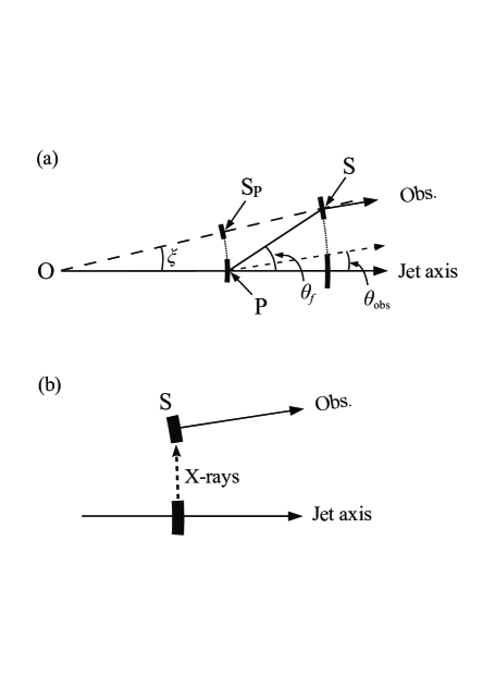
Figure 1: Case 1. (a) The jet is ejected from O and consists of patchy regions, and they move radially with Lorentz factor $\Gamma$. The primary flare occurs at P. During time interval $\delta t$, the dense region around S_P moves to S and a fraction of X-rays emitted at P travels toward S. Then the secondary (“orphan”) flare is triggered at S. The observer is located at angle $\theta_{\mathrm{obs}}=\eta/\Gamma$ off the jet axis, and the points S_P and S are on the line at angle $\xi=\alpha/\Gamma$ off the jet axis. The distances OP and OS_P are $d$, $\mathrm{S}_{\mathrm{P}}\mathrm{S}=\beta c\delta t$, and $\mathrm{PS}=c\delta t$. (b) Emission regions in the comoving frame of the jet. X-rays emitted in the primary flare are injected into S and they are scattered by nonthermal particles in S.

We first study the kinematics of a jet shown in Figure 1 (Case 1). We assume that a jet (a patchy plasma shell) with bulk Lorentz factor $\Gamma$ is ejected radially from point O that is close to the central black hole. The observer is at angle $\theta_{\mathrm{obs}}=\eta/\Gamma$ from the jet axis, where $\eta\sim{\cal O}(1)$. At P the primary flare occurs, which is triggered by, e.g., the internal shock. Here we assume that the high energy particles are confined in a patchy shell and high density regions are located at P and S_P in the shell. The emission mechanisms in a flare are synchrotron emission and SSC for X-rays and TeV $\gamma$-rays, respectively. A fraction of the emitted photons propagate along directions that are slightly off from the jet axis and they are injected into the high density region around S, where S was located at S_P when the primary flare occurred. The injected TeV $\gamma$-rays are in Klein-Nishina regime and are not scattered but X-rays are Compton-scattered to become TeV $\gamma$-rays. This triggers the secondary (OTG) flare in the TeV region.

We assume that the photons emitted at P reach S after time interval $\delta t$ in the rest frame of the black hole and that the propagation direction of those photons is denoted by $\theta_{f}$. For the geometry shown in Figure 1, equations to be solved for $\delta t$ and $\theta_{f}$ for given $d$, $\xi$, and $\Gamma$ are as follows:

$$(d+\beta\,c\,\delta t)\sin\xi=c\,\delta t\,\sin\theta_{f},$$ (1)

and

$$(d+\beta\,c\,\delta t)^{2}=d^{2}+(c\,\delta t)^{2}-2\,d\,c\,\delta t\,\cos(\pi-\theta_{f}),$$ (2)

where $c$ is the light speed and $\beta=\sqrt{1-1/\Gamma^{2}}$. Here we assumed that the distances between O and P, OP, and O and S_P, OS_P, are the same, i.e., $\mathrm{OP}=\mathrm{OS}_{\mathrm{P}}=d$. Next we assume that $\xi=\alpha/\Gamma$, where $\alpha\sim{\cal O}(1)$ is a constant. Using equations (1) and (2), we obtain the equation for $x\equiv c\delta t/d$:

$$x^{2}+4\Gamma\sqrt{\Gamma^{2}-1}\left(\frac{2\alpha^{2}}{x}-x\right)+\frac{4\alpha^{2}\Gamma^{2}}{x^{2}}-4\alpha^{2}+4(\alpha^{2}-1)\Gamma^{2}=0.$$ (3)

There are four solutions for $x$, but the physically allowed solution is unique and given by

$$x = \Gamma\sqrt{\Gamma^{2}-1}-\sqrt{\Gamma^{4}-(1+\alpha^{2})\Gamma^{2}+\alpha^{2}}$$ (4)

$$+\left\{2\Gamma^{4}-\alpha^{2}(\Gamma^{2}-1)+\frac{2\Gamma^{3}(\Gamma^{2}-1)^{1/2}}{[\Gamma^{4}-(1+\alpha^{2})\Gamma^{2}+\alpha^{2}]^{1/2}}(\alpha^{2}-\Gamma^{2})\right\}^{1/2}.$$

When $\Gamma\gg 1$, $c\,\delta t/d$ is approximated as

$$\frac{c\,\delta t}{d}\approx\frac{\alpha^{2}}{2}+\sqrt{\alpha^{2}+\frac{\alpha^{4}}{4}}+{\cal O}(\Gamma^{-2}).$$ (5)

From equation (1) we obtain

$$\sin\theta_{f}\approx\frac{1}{\Gamma}\left[\alpha+\frac{2}{\alpha+\sqrt{4+\alpha^{2}}}\right].$$ (6)

Because the angle between the jet axis and the line of sight is $\theta_{\mathrm{obs}}$, the observed delay time of the secondary flare from the primary flare is given by

$$\delta t_{\mathrm{obs}}=[1-\cos(\theta_{f}-\theta_{\mathrm{obs}})]\,\delta t\approx\frac{1}{\Gamma^{2}}\,f(\alpha)\,\frac{d}{c}\,,$$ (7)

where

$$f(\alpha)=\frac{1}{4}\left(\alpha^{2}+\sqrt{\alpha^{2}+\frac{\alpha^{4}}{4}}\right)\left[2+\alpha^{2}+\sqrt{4\alpha^{2}+\alpha^{4}}-\alpha\eta\left(4+\frac{8}{\alpha^{2}+\sqrt{4\alpha^{2}+\alpha^{4}}}\right)+2\eta^{2}\right].$$ (8)

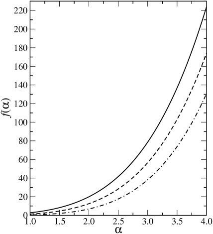
Figure 2: $f(\alpha)$ for $\eta=0$ (solid), 0.5 (dashed), and 1 (dot-dashed).

The behavior of $f(\alpha)$ is shown in Figure 2. For example, $f\approx 38.2$ for $\alpha=3$ and $\eta=1$. Note the strong dependence of $f$ on $\alpha$. The numerical value of $\delta t_{\mathrm{obs}}$ is estimated as

$$\delta t_{\mathrm{obs}}\approx 0.29\left(\frac{20}{\Gamma}\right)^{2}\left(\frac{d}{3\times 10^{17}\,\mathrm{cm}}\right)f(\alpha)\quad\mathrm{days}.$$ (9)

Then $\delta t_{\mathrm{obs}}\approx 15$ days is obtained for $\Gamma=20$, $d=4\times 10^{17}$ cm, $\eta=1$, and $\alpha=3$. This value is close to the observed delay time of the OTG flare in 1ES 1959+650 (Krawczynski et al., 2004). These parameters give the distance of S from the central black hole $d+\beta c\delta t\approx 1.4$ pc.

There is another possibility of the jet geometry (Case 2) as shown in Figure 3. Here we assume that the X-ray source is located at P that is away from the jet axis and that the secondary flare occurs at S_P on the jet axis. The solution for $c\delta t/d$ is the same as equation (5) and $\theta_{f}$ is given by equation (6). If a flare at S_P occurs simultaneously with a flare at P and the flare at S_P is observed, the observed time delay between the flares at S_P and S is given by

$$\delta t_{\mathrm{obs}}=(1-\beta\cos\theta_{\mathrm{obs}})\delta t\approx\frac{1}{\Gamma^{2}}\,f_{1}(\alpha)\,\frac{d}{c},$$ (10)

where

$$f_{1}(\alpha)=\left(\frac{\alpha^{2}}{2}+\sqrt{\alpha^{2}+\frac{\alpha^{4}}{4}}\right)\frac{1+\eta^{2}}{2}.$$ (11)

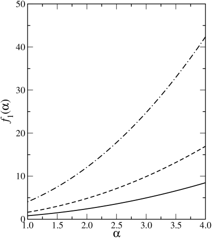
Figure 4: $f_{1}(\alpha)$ for $\eta=0$ (solid), 1 (dashed), and 2 (dot-dashed).

The values of $f_{1}(\alpha)$ for $\eta=0$, 1, and 2 are shown in Figure 4. If $\Gamma=20$, $\alpha=3$, $\eta=1$, and $d=4\times 10^{17}$ cm are assumed, the delay time is about 4 days and too short to explain the observed delay time. If $\eta$ is larger, the delay time becomes larger, but the observed luminosity decreases significantly because of the beaming effects.

If the primary flare at P is observed and a flare at S_P is not observed, the delay time between the flares at P and S is given by

$$\delta t_{\mathrm{obs}}=\cases{[1-\cos(\theta_{\mathrm{obs}}-\xi+\theta_{f})]\delta t\approx\frac{\displaystyle 1}{\displaystyle\Gamma^{2}}\,f_{2}(\alpha)\,\frac{\displaystyle d}{\displaystyle c}&if $\xi<\theta_{\mathrm{obs}}$\cr(1-\cos\theta_{f})\delta t\approx\frac{\displaystyle 1}{\displaystyle\Gamma^{2}}\,f_{3}(\alpha)\,\frac{\displaystyle d}{\displaystyle c}&if $\xi>\theta_{\mathrm{obs}}$ ,}$$ (12)

where

$$f_{2}(\alpha)=4\alpha\eta+\alpha^{2}(\eta^{2}-1)+\alpha\sqrt{4+\alpha^{2}}(1+\eta^{2}),$$ (13)

and

$$f_{3}(\alpha)=\frac{\alpha^{4}+3\alpha^{2}}{4}+\frac{1+\alpha^{2}}{2}\sqrt{\alpha^{2}+\frac{\alpha^{4}}{4}}.$$ (14)

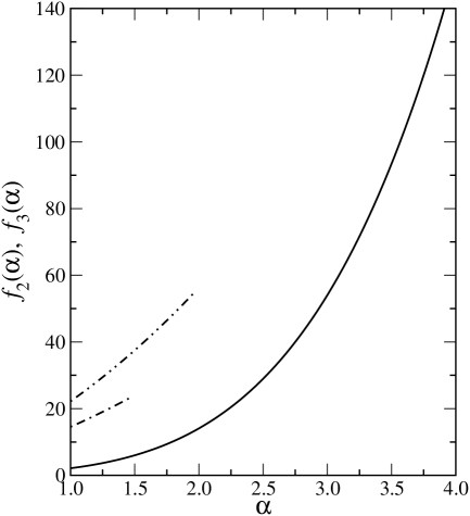
Figure 5: $f_{2}(\alpha)$ for $\eta=1.5$ (dot-dashed) and 2 (dot-dot-dashed) and $f_{3}(\alpha)$ (solid). $f_{2}(\alpha)$ and $f_{3}(\alpha)$ are used to calculate $\delta t_{\mathrm{obs}}$ in Eq. (12) for $\alpha<\eta$ and $\alpha>\eta$, respectively.

$f_{2}(\alpha)$ for $\eta=1.5$ and 2 and $f_{3}(\alpha)$ are shown in Figure 5. When $\xi<\theta_{\mathrm{obs}}$, $\eta\gtrsim 1.5$ and $\alpha\gtrsim 1.5$ are needed to obtain $\delta t_{\mathrm{obs}}\sim$ 2 weeks, if $\Gamma=20$ and $d=4\times 10^{17}$ cm are assumed. When $\xi>\theta_{\mathrm{obs}}$, $\alpha\gtrsim 2.7$ is required to explain $\delta t_{\mathrm{obs}}\sim$ 2 weeks for the same parameter values as the above.

3 Properties of the Secondary Flare

3.1 Timescales

The solution obtained in §2 gives the distance, S_PS, that the emission region travels during $\delta t$ as

$$\beta c\delta t\sim\left(\frac{\alpha^{2}}{2}+\sqrt{\alpha^{2}+\frac{\alpha^{4}}{4}}\right)d.$$ (15)

In the comoving frame of the jet, the travel time is given by

$$\delta t^{\prime}\sim\frac{\delta t}{\Gamma}\approx 57.9\left(\frac{\alpha^{2}}{2}+\sqrt{\alpha^{2}+\frac{\alpha^{4}}{4}}\right)\left(\frac{20}{\Gamma}\right)\left(\frac{d}{3\times 10^{17}\mathrm{cm}}\right)\quad\mathrm{days}.$$ (16)

If $\alpha=3$, we obtain $\delta t^{\prime}\sim 574$ days. Here primed quantities are evaluated in the comoving frame of the jet.

Synchrotron cooling rate per electron in the comoving frame of the jet is given by $P^{\prime}_{\mathrm{syn}}=(4/3)\sigma_{\mathrm{T}}c\beta^{\prime\,2}\gamma^{\prime\,2}u^{\prime}_{B}$, where $u^{\prime}_{B}$ is the magnetic energy density. Then we obtain the cooling time as $t^{\prime}_{\mathrm{syn}}=\gamma^{\prime}m_{e}c^{2}/P^{\prime}_{\mathrm{syn}}$. The characteristic energy of synchrotron radiation is given by $\epsilon^{\prime}_{\mathrm{syn}}=3\hbar eB^{\prime}\gamma^{\prime\,2}/(2m_{e}c)$ and the observed synchrotron photon energy is Doppler shifted, i.e., $\epsilon_{\mathrm{syn}}\sim\Gamma\epsilon^{\prime}_{\mathrm{syn}}$. Because synchrotron photons with energy $\epsilon^{\prime}_{\mathrm{syn}}$ are emitted by electrons with a Lorentz factor

$$\gamma^{\prime}\sim 5.37\times 10^{5}\left(\frac{B^{\prime}}{0.1\mathrm{G}}\right)^{-1/2}\,\left(\frac{\Gamma}{20}\right)^{-1/2}\,\left(\frac{\epsilon_{\mathrm{syn}}}{10\mathrm{keV}}\right)^{1/2},$$ (17)

we obtain

$$t^{\prime}_{\mathrm{syn}}\sim 1.7\left(\frac{B^{\prime}}{0.1\mathrm{G}}\right)^{-3/2}\left(\frac{\Gamma}{20}\right)^{1/2}\left(\frac{\epsilon_{\mathrm{syn}}}{10\mathrm{keV}}\right)^{-1/2}\quad\mathrm{days}.$$ (18)

Then we find that $t^{\prime}_{\mathrm{syn}}<\delta t^{\prime}$. Because the cooling by inverse Compton scattering is not negligible, the cooling time is much shorter than $t^{\prime}_{\mathrm{syn}}$. Thus relativistic electrons/positrons injected into the primary flare are already cooled when the secondary flare occurs. For the secondary flare to be caused, the injection of relativistic electrons/positrons is necessary. The injection rate, however, does not need to be as high as in the primary flare. When synchrotron photons from the primary flare impinge on the dense region, which is located at the right place as described in §2, the secondary flare occurs by inverse Compton scattering of those photons.

3.2 Beaming effects

There is a slight velocity difference between S_P and P. The relative velocity between points S_P and P normalized by the light speed is given by $\beta_{\mathrm{rel}}=2\beta\sin(\xi/2)\approx\alpha\beta/\Gamma$. Thus the relative velocity is negligible for $\Gamma\gg 1$ and points S_P and P are safely assumed to be in the same inertial frame. The observed luminosity of TeV $\gamma$-rays from S is enhanced by a factor ${\cal D}_{\xi}^{4}$ because of the relativistic effects in Case 1, where

$$D_{\xi} = \frac{1}{\Gamma[1-\beta\cos(\xi-\theta_{\mathrm{obs}})]}$$ (19)

$$\approx \frac{2}{1+(\alpha-\eta)^{2}}\,\Gamma+\frac{(\alpha-\eta)^{4}+6(\alpha-\eta)^{2}-3}{6[1+(\alpha-\eta)^{2}]^{2}}\,\frac{1}{\Gamma}+{\cal O}(\Gamma^{-3}).$$ (20)

In Case 1, the ratio of the luminosity enhancements by the beaming effects at S and P is $r=(D_{\xi}/D_{\mathrm{obs}})^{4}=\{(1+\eta^{2})/[1+(\alpha-\eta)^{2}]\}^{4}$, where

$$D_{\mathrm{obs}}=\frac{1}{\Gamma(1-\beta\cos\theta_{\mathrm{obs}})}\approx\frac{2}{1+\eta^{2}}\,\Gamma+\frac{\eta^{4}+6\eta^{2}-3}{6(1+\eta^{2})^{2}}\,\frac{1}{\Gamma}+{\cal O}(\Gamma^{-3}).$$ (21)

If $\alpha=3$ and $\eta=1$, $r\approx 1/40$. In Case 2, $r=(D_{\mathrm{obs}}/D_{\xi})^{4}\approx 40$.

4 Summary and Discussion

In this paper we have proposed a structured jet model for the OTG flares. The high energy emission spectra from TeV blazars have been well explained by the leptonic jet models. Because the leptonic jet models assume synchrotron self-Compton scattering for the emission mechanism of very high energy $\gamma$-rays, it is expected that flares occur in both X-ray and $\gamma$-ray energy bands almost simultaneously. However, the OTG flares were not accompanied by the simultaneous increase in the X-ray flux (Krawczynski et al., 2004; Błażejowski et al., 2005), and this is thought to be a challenging issue for the leptonic jet models. Our model of a structured jet assumes that $\gamma$-rays are emitted in different components in the jet. X-rays produced by a flare in a region, where flares in X-rays and TeV $\gamma$-rays occur simultaneously, are scattered in another region of the jet and the scattered photons are observed as a secondary (OTG) flare. Note that TeV $\gamma$-rays of the primary flare are not scattered by electrons/positrons because of Klein-Nishina effects. The emitted $\gamma$-ray energy is estimated as $\epsilon^{\prime}_{\mathrm{SSC}}=\gamma^{\prime}m_{e}c^{2}$, because the scattering occurs mainly in Klein-Nishina regime. Then the observed $\gamma$-ray energy is roughly given by

$$\epsilon_{\mathrm{SSC}}\sim\Gamma\epsilon^{\prime}_{\mathrm{SSC}}\sim 5.5\times 10^{12}\left(\frac{B^{\prime}}{0.1\mathrm{G}}\right)^{-1/2}\left(\frac{\Gamma}{20}\right)^{1/2}\left(\frac{\epsilon_{\mathrm{syn}}}{10\mathrm{keV}}\right)^{1/2}\quad\mathrm{eV},$$ (22)

using equation (17).

Because the X-rays emitted in the primary flare need a propagation time before they are scattered in different parts of the jet, this results in the time delay between the primary and secondary flares. In our model, the delay time between the primary flare and the secondary TeV $\gamma$-ray flare is dependent on $\Gamma$, $\alpha$, $\eta$, and $d$. The observed delay time is about 15 days for 1ES 1959+650 and this value is obtained for $\Gamma=20$, $\alpha=3$, $\eta=1$, and $d=4\times 10^{17}$ cm in Case 1. As the value of $\alpha$ decreases the value of $d$ increases for a given value of $\delta t_{\mathrm{obs}}$. If the value of $\Gamma$ is known from the observations of the primary flare, the values of $\alpha$ and $d$ might be reasonably guessed from the delay time. It is not clear from the numerical values estimated in this paper whether Case 1 is favored to Case 2 or vice versa. Rare observations of OTG flares might be due to that this phenomenon needs a specific structure of the jets as shown in Figures 1 or 3.

The duration of the secondary flare depends on the time interval of the primary flare and the angular size of the secondary flare site, $\Delta\theta$. For example, in Case 1, if $\Delta\theta$ is given by $\Delta\alpha/\Gamma$ and the primary flare is impulsive, the observed duration of the second flare is given by the difference between the values of $\delta t_{\mathrm{obs}}$ for $\alpha$ and $\alpha+\Delta\alpha$:

$$t_{\mathrm{dur}}\approx 0.29\left(\frac{20}{\Gamma}\right)^{2}\left(\frac{d}{3\times 10^{17}\,\mathrm{cm}}\right)\frac{df(\alpha)}{d\alpha}\Delta\alpha\quad\mathrm{days},$$ (23)

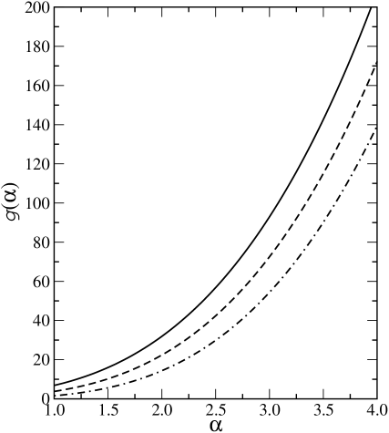
Figure 6: $g(\alpha)$ for $\eta=0$ (solid), 0.5 (dashed), and 1 (dot-dashed).

where $\Delta\alpha\ll 1$ is assumed. The values of $g(\alpha)=df/d\alpha$ are shown in Figure 6 for Case 1. For example, $g\approx 54.4$ for $\eta=1$ and $\alpha=3$. If the observed duration of the secondary flare is about 5 hours, $\Delta\alpha\sim 0.01$ for $\alpha=3$, $\Gamma=20$, and $d=4\times 10^{17}$ cm. The observed duration of the secondary flare may depend on not only the value of $\Delta\alpha$ but also the duration of the primary flare, and the effect of the latter elongates the duration of the secondary flare.

We have shown that the time lag between the primary and secondary flares are well accounted for by our model. Next we argue that the density of soft photons (X-rays) from the primary flare is high enough to produce the OTG flare if the particle injection time in the primary flare is sufficiently long, and that the particle injection rate needed in the secondary flare is not unreasonably high.

First, it should be noted that photons from the primary flare blob (PB) are not injected from the rear side of the secondary flare blob (SB). In the comoving frame of the blobs, the angle between the line of sight and the incident direction of photons from PB is about 90 degrees. Then the energy boost by inverse Compton scattering in SB should be effective, although the detailed calculations of radiative transfer are necessary to obtain the emission spectrum of TeV $\gamma$-rays from SB.

Next, we discuss the amount of radiation received by SB and the cooling time of leptons. In the following, primed symbols are quantities during the primary flare in the comoving frame and doubly primed symbols are quantities during the secondary flare in the comoving frame. We assume that PB and SB are spherical plasma clouds for simplicity. The radii of PB and SB in the comoving frame at the occurrence of the primary flare are denoted by $R^{\prime}_{\mathrm{prim}}$ and $R^{\prime}_{\mathrm{sec}}$, respectively. The radius of SB at the time when the secondary flare occurs is denoted by $R^{\prime\prime}_{\mathrm{sec}}$. The solid angle extended by SB for a point in PB is given by $\Omega^{\prime}_{\mathrm{sec}}\sim\pi R^{\prime\,2}_{\mathrm{sec}}/d^{\prime\,2}_{\mathrm{sec}}$, where $d^{\prime}_{\mathrm{sec}}$ is the distance between PB and SB: $d^{\prime}_{\mathrm{sec}}\sim\xi d=(\alpha/\Gamma)\,d$. If SB expands proportionally with the distance from the central black hole, $\Omega^{\prime}_{\mathrm{sec}}=\Omega^{\prime\prime}_{\mathrm{sec}}$. If radiation from PB is emitted isotropically in the comoving frame, the fraction of the radiation received by SB is given by

$$r_{\mathrm{rad}}\equiv\frac{\Omega^{\prime}_{\mathrm{sec}}}{4\pi}=\frac{1}{4}\,\frac{\Gamma^{2}}{\alpha^{2}}\,\frac{R^{\prime\,2}_{\mathrm{sec}}}{d^{2}}\sim\frac{1}{36}\left(\frac{\Gamma}{20}\right)^{2}\left(\frac{3}{\alpha}\right)^{2}\left(\frac{R^{\prime}_{\mathrm{sec}}}{2\times 10^{16}\mathrm{cm}}\right)^{2}\left(\frac{4\times 10^{17}\mathrm{cm}}{d}\right)^{2}.$$ (24)

We assumed $R^{\prime}_{\mathrm{sec}}\sim 2\times 10^{16}$ cm; this value is close to the values assumed for the emission region of the flare models of 1ES 1959+650 in Krawczynski et al. (2004). Thus the soft photon (X-ray) energy density in SB is roughly about 1/30 of that in PB and the Compton cooling time of nonthermal particles in SB is longer by 30 times than in PB. On the other hand, the flare duration in PB is determined by the injection duration of nonthermal particles, because the cooling time should be short owing to the large energy densities of soft photons and magnetic fields. Thus the observed OTG flare is explained, if the particle injection duration in PB is about 30 times longer than the cooling time in SB. Furthermore, the energy densities of magnetic fields and internal synchrotron photons in SB are smaller than in PB, so that emission other than TeV $\gamma$-rays is too weak to be observed.

In the following we estimate the required injection rate of nonthermal leptons in the secondary flare. The observed energy flux of the secondary flare at 600GeV is $\nu F_{\nu}\sim 3\times 10^{-10}$ ergs s^-1 cm^-2. The luminosity distance to 1ES 1959+650 ($z=0.047$) is $d_{L}=210$ Mpc, assuming that $H_{0}=70$ km s^-1 Mpc^-1, $\Omega_{\Lambda}=0.7$, and $\Omega_{m}=0.3$, where $H_{0}$, $\Omega_{\Lambda}$, and $\Omega_{m}$ are the Hubble constant and the density parameters of dark energy and matter, respectively. Then the luminosity of the very high energy gamma-rays is $L_{\mathrm{VHE,sec}}\sim 1.6\times 10^{45}$ ergs s^-1. The luminosity in the comoving frame is given by

$$L^{\prime\prime}_{\mathrm{VHE,sec}}=\frac{L_{\mathrm{VHE,sec}}}{{\cal D}^{4}_{\mathrm{sec}}}\sim 9.9\times 10^{39}\left(\frac{{\cal D}_{\mathrm{sec}}}{20}\right)^{-4}\quad\mathrm{ergs}\,\mathrm{s}^{-1},$$ (25)

where ${\cal D}_{\mathrm{sec}}$ is the beaming factor of SB and ${\cal D}_{\mathrm{sec}}=8$ and 20 for Cases 1 and 2, respectively, if $\Gamma=20$, $\alpha=3$, and $\eta=1$. The distance between the central black hole and SB is $d_{\mathrm{sec}}=d+\beta c\delta t\sim 11d$, where $\alpha=3$ is assumed. Assume that SB expands linearly with the distance from the central black hole. Then the radius of SB is given by

$$R^{\prime\prime}_{\mathrm{sec}}=\frac{d_{\mathrm{sec}}}{d}\,R^{\prime}_{\mathrm{sec}}\sim 11R^{\prime}_{\mathrm{sec}}=2.2\times 10^{17}\left(\frac{R^{\prime}_{\mathrm{sec}}}{2\times 10^{16}\mathrm{cm}}\right)\quad\mathrm{cm}.$$ (26)

We obtain the energy injection rate per unit volume during the secondary flare:

$$q^{\prime\prime}_{\mathrm{sec}}=\frac{L^{\prime\prime}_{\mathrm{VHE,sec}}}{\frac{4\pi}{3}R^{\prime\prime\,3}_{\mathrm{sec}}}=2.2\times 10^{-13}\left(\frac{R^{\prime}_{\mathrm{sec}}}{2\times 10^{16}\mathrm{cm}}\right)^{-3}\left(\frac{{\cal D}_{\mathrm{sec}}}{20}\right)^{-4}\quad\mathrm{ergs}\,\mathrm{s}^{-1}\,\mathrm{cm}^{-3}.$$ (27)

The injection rate of nonthermal leptons in SB is also given by

$$N^{\prime\prime}_{e}=\frac{L^{\prime\prime}_{\mathrm{VHE,sec}}}{\langle\gamma\rangle m_{e}c^{2}}=2.4\times 10^{40}\left(\frac{{\cal D}_{\mathrm{sec}}}{20}\right)^{-4}\left(\frac{\langle\gamma\rangle}{5\times 10^{5}}\right)^{-1}\quad\mathrm{s}^{-1},$$ (28)

where $\langle\gamma\rangle$ is the value of the characteristic Lorentz factor of injected leptons in SB. When the energy injection rate during the primary flare is denoted by $q^{\prime}_{\mathrm{prim}}$, we obtain

$$\frac{q^{\prime\prime}_{\mathrm{sec}}}{q^{\prime}_{\mathrm{prim}}}=\frac{L^{\prime\prime}_{\mathrm{VHE,sec}}/\left(\frac{4\pi}{3}R^{\prime\prime\,3}_{\mathrm{sec}}\right)}{L^{\prime}_{\mathrm{VHE,prim}}/\left(\frac{4\pi}{3}R^{\prime\,3}_{\mathrm{prim}}\right)}=\frac{[\nu F_{\nu}]_{\mathrm{VHE,sec}}}{[\nu F_{\nu}]_{\mathrm{VHE,prim}}}\left(\frac{{\cal D}_{\mathrm{prim}}}{{\cal D}_{\mathrm{sec}}}\right)^{4}\left(\frac{R^{\prime}_{\mathrm{prim}}}{R^{\prime\prime}_{\mathrm{sec}}}\right)^{3},$$ (29)

where $[\nu F_{\nu}]_{\mathrm{VHE,prim}}$ and $[\nu F_{\nu}]_{\mathrm{VHE,sec}}$ are the observed quantities of $\nu F_{\nu}$ in the primary and secondary flares, respectively. If $R^{\prime}_{\mathrm{sec}}\sim R^{\prime}_{\mathrm{prim}}$ and $R^{\prime\prime}_{\mathrm{sec}}\sim 11R^{\prime}_{\mathrm{sec}}$ are assumed, $q^{\prime\prime}_{\mathrm{sec}}/q^{\prime}_{\mathrm{prim}}\sim c_{1}\,[\nu F_{\nu}]_{\mathrm{VHE,sec}}/[\nu F_{\nu}]_{\mathrm{VHE,prim}}$, where $c_{1}\sim 3.0\times 10^{-2}$ and $1.9\times 10^{-5}$ for Cases 1 and 2, respectively. From the observed data (Krawczynski et al., 2004), we may set
$[\nu F_{\nu}]_{\mathrm{VHE,sec}}/[\nu F_{\nu}]_{\mathrm{VHE,prim}}\sim 1$, and $q^{\prime\prime}_{\mathrm{sec}}\sim c_{1}q^{\prime}_{\mathrm{prim}}$ is obtained. Thus the required value of $q^{\prime\prime}_{\mathrm{sec}}$ is not unreasonably large. This particle energy is transfered to X-rays by inverse Compton scattering to emit TeV $\gamma$-rays in the secondary flare.

Our model assumes a structured jet and the occurrence of OTG flares depends on the geometry of dense regions in the jet. Alternatively the dense regions might be widely distributed, e.g., the layer-spine model by Ghisellini et al. (2005), and the value of $\alpha$ depends on where the region of particle acceleration at pc-scale exists.

Finally we comment on the observed large scale structure of jets. The line of sight is inside the opening angle of jets in our model, and this may result in a core-halo structure of the emission region. However, since the emission regions of high energy radiation are located very close to the central black hole, the large scale structure of jets is affected by the environment of the jets. That is, the interaction between jets and gases surrounding the central region may cause the bending of the jets. It is also possible that the opening angle may change with the distance from the central region. These may account for the jet structure observed by VLBI.

Figure 3: Case 2. Same as Fig. 1 except that X-rays come from the off-axis region around P.

References

- Aharonian (2004) Aharonian, F. A. 2004, Very High Energy Cosmic Gamma Radiation (Singapore: World Scientific)
- Aharonian et al. (2005) Aharonian, F. A., et al. 2005, A&A, 441, 465
- Błażejowski et al. (2005) Błażejowski, M., et al. 2005, ApJ, 630, 130
- Böttcher (2005) Böttcher, M., 2005, ApJ, 621, 176 [Erratum: 2006, ApJ, 641, 1233]
- Daniel et al. (2005) Daniel, M. K., et al. 2005, ApJ, 621, 181
- Ghisellini et al. (2005) Ghisellini, G., Tavecchio, F., & Chiaberge, M. 2005, A&A, 432, 401
- Hartman et al. (1999) Hartman, R. C., et al. 1999, ApJS, 123, 79
- Krawczynski (2004) Krawczynski, H. 2004, New Astronomy Rev., 48, 367
- Krawczynski et al. (2004) Krawczynski, H., et al. 2004, ApJ, 601, 151
- Kusunose et al. (2000) Kusunose, M., Takahara, F., & Li, H. 2000, ApJ, 536, 299
- Li & Kusunose (2000) Li, H., & Kusunose, M. 2000, ApJ, 536, 729
- Maraschi et al. (1992) Maraschi, L., Ghisellini, G., & Celotti, A. 1992, ApJ, 397, L5
- Mastichiadis & Kirk (1997) Mastichiadis, A., & Kirk, J. G. 1997, A&A, 320, 19
- Reimer et al. (2005) Reimer, A., Böttcher, M., & Postnikov, S. 2005, ApJ, 630, 186