Shear Recovery Accuracy in Weak Lensing Analysis with
Elliptical Gauss-Laguerre Method

Abstract

We implement the Elliptical Gauss-Laguerre (EGL) galaxy-shape measurement method proposed by Bernstein & Jarvis (2002) [BJ (02)] and quantify the shear recovery accuracy in weak lensing analysis. This method uses a deconvolution fitting scheme to remove the effects of the point-spread function (PSF). The test simulates $>10^{7}$ noisy galaxy images convolved with anisotropic PSFs, and attempts to recover an input shear. The tests are designed to be immune to shape noise, selection biases, and crowding. The systematic error in shear recovery is divided into two classes, calibration (multiplicative) and additive, with the latter arising from PSF anisotropy. At S/N $>50$, the deconvolution method measures the galaxy shape and input shear to $\sim 1\%$ multiplicative accuracy, and suppresses $>99\%$ of the PSF anisotropy. These systematic errors increase to $\sim 4\%$ for the worst conditions, with poorly resolved galaxies at S/N $\simeq 20$. The EGL weak lensing analysis has the best demonstrated accuracy to date, sufficient for the next generation of weak lensing surveys.

1 Introduction

Weak gravitational lensing, the shearing of galaxy images by gravitational bending of light, is an effective tool to probe the large-scale matter distribution of the universe. It is also a means to measure the cosmological parameters by comparing observation to numerical simulations of large scale structure growth (Bartelmann & Schneider, 2001). There are many weak lensing (WL) surveys underway to obtain the cosmological parameters to higher precision, and in particular to probe the evolution of the dark energy by observing its effects on the evolution of matter distribution (DLS, CFHTLS).

The WL signal is very subtle, however; it is necessary to measure these small distortions (typical shear $\gamma\sim 1\%$) in the presence of optical distortions and the asymmetric point-spread-function (PSF) of real-life imaging. The level of systematic error in the WL measurement methods are currently above the statistical accuracy expected from future wide and deep WL surveys (Pan-STARRS, SNAP, LSST, SKA). Because there are no “standard shear” lenses on the sky, shear-measurement techniques are tested by applying them to artificial galaxy images and seeing if one can correctly extract a shear applied to the simulation. In most cases, the recovered shear can be written as $\gamma_{\rm out}=m\gamma_{\rm in}+c$. Departures from the ideal $m=1$ we will term “calibration” or “multiplicative” errors and quote as percentages. Deviations from the ideal $c=0$ can result from uncorrected asymmetries in the PSF and optics, and will be termed “additive errors” or “incomplete PSF suppression.”

Such tests of the most widely applied analysis method (Kaiser, Squires, & Broadhurst, 1995)[KSB], find $m=$0.8–0.9, but this coefficient is implementation dependent (Erben et al., 2001; Bacon et al., 2001), and depends upon the characteristics of the simulated galaxies. Hirata & Seljak (2003) [HS (03)] demonstrate that various PSF-correction methods can produce shear measurements miscalibrated by a few % to 20% or more. Heymans et al. (2005) [Shear TEsting Programme, (STEP )] present testing of many existing shear-measurement pipelines using a common ensemble of sheared simulated images. These methods show a median calibration error of 7%, although some (the BJ02 rounding kernel method, an implementation of a KSB method, as well as the one described in this paper) show no calibration error, to within the $\sigma_{m}\approx 1\%$ noise level of the first STEP tests. Although the statistical accuracy in past surveys was comparable to the 7% systematics, it is expected to be well below 1% in future surveys. Hence, understanding and eliminating the WL systematic errors require the most urgent attention today.

In this paper, we implement the elliptical Gauss-Laguerre (EGL) deconvolution method as described in BJ02, and subject it to a series of tests designed to be more stringent than any previous test of WL measurements. The deconvolution method is distinct from the Jarvis et al. (2003) method, also described BJ02, in which the anisotropic PSF effects are removed using a “rounding kernel” instead.

WL testing regimes are of two types: in end-to-end tests (e.g. STEP), one produces simulated sky images with a full population of stars and galaxies, analyzes them with the same pipeline as one would real data, then checks the output shear for veracity. We perform here more of a dissection, in which we analyze the performance of the method one galaxy type at a time, and vary the parameters of the galaxy and PSF images to determine which, if any, conditions cause the measurement to fail. While lacking the realism of an end-to-end test, this allows us to isolate and fix weaknesses. If we can demonstrate that the method succeeds under a set of conditions that will circumscribe those found on the real sky, then we can have confidence that our method is reliable, whereas end-to-end testing is reliable only to the extent that the simulated sky reproduces the characteristics of the real sky.

We investigate here the performance of our EGL method across the range of noise levels, degree of resolution by the PSF, pixel sampling rates, galaxy ellipticity, and PSF ellipticity, using both highly symmetric and asymmetric galaxy shapes. We test not only the accuracy of shear recovery, but also the accuracy of the shear uncertainty estimates.

The EGL method is further elaborated in §2, while the implementation, GLFit, is detailed in §3. The shear accuracy test procedure is described in §4. The conditions under which the shape measurement succeeds, and the accuracy of its estimates of shear, are presented in §5. Previous dissection tests include HS (03) and Kuijken (2006). The former studies the performance of several methodologies on varied galaxy and PSF shapes/sizes in the absence of noise. The latter study verified its “polar shapelet” method to better than 1% calibration accuracy. In §6 and §7 we conclude with comparisons to other shape-measurement methodologies and tests, and draw inferences for future surveys.

2 Overview of Shape Measurement

The task of this weak lensing methodology is to assign some shape $\mbox{\boldmath$e$}_{i}$ to observed galaxy $i$, then to derive from the ensemble $\{\mbox{\boldmath$e$}_{i}\}$ an estimate of the applied lensing shear $\gamma$. More precisely, a shape analysis can only determine the reduced shear $g=\gamma/(1-\kappa)$, where $\kappa$ is the lens convergence. Following BJ02, we use distortion $\delta$ to describe the shear, where $\delta=2g/(1+g^{2})$ ($\delta\simeq 2g$ for $g\ll 1$). In this paper, both the shear and the shapes are expressed as distortions; while in other WL literatures, shear is usually expressed as $g$.

2.1 Defining Shapes using Shear

Following BJ02, we will quantify the lensing by decomposing its magnification matrix ${\bf M}$ into a diagonal dilation matrix ${\bf D}_{\mu}=e^{\mu}{\bf I}$ and a unit-determinant symmetric shear matrix ${\bf S}_{\mbox{\boldmath$\eta$}}$:

$${\bf M} = {\bf D_{\mu}}{\bf S}_{\mbox{\boldmath$\eta$}}={\bf D_{\mu}}{\bf R}_{\beta}{\bf S}_{\eta}{\bf R}_{-\beta}$$ (1)

$${\bf R}_{\beta} = \left(\begin{array}[]{cc}\cos\beta&-\sin\beta\\ \sin\beta&\cos\beta\end{array}\right)$$ (4)

$${\bf S}_{\eta} = \left(\begin{array}[]{cc}e^{\eta/2}&0\\ 0&e^{-\eta/2}\end{array}\right)$$ (7)

$$\eta \equiv (\eta_{+},\eta_{\times})=(\eta\cos 2\beta,\eta\sin 2\beta)$$ (8)

where $\beta$ is the direction of the shear axis, and $\eta$ is a measure of shear. The “conformal shear” $\eta$ can be reparameterized as the distortion $\delta=\tanh\eta$ or the reduced shear $g=\tanh\eta/2$.

The shape must be assigned to an image of a galaxy with some surface-brightness distribution $I(\mbox{\boldmath$\theta$})$. Initially we will ignore the effects of PSF convolution on the observed image. The BJ02 definition of shape is to specify roundness criteria or “circularity tests,” $M_{+}(I)$ and $M_{\times}(I)$, that operate on $I$ to yield one scalar for each component of the shear—typically these are quadrupole moments. The object is deemed circular ($\mbox{\boldmath$e$}=0$) if $M_{+}(I)=M_{\times}(I)=0$. If the object is not circular, then we assign to the object the shape $\eta$ which yields the solutions

$$M_{+}[I({\bf S}_{\mbox{\boldmath$\eta$}}\mbox{\boldmath$\theta$})]=M_{\times}[I({\bf S}_{\mbox{\boldmath$\eta$}}\mbox{\boldmath$\theta$})]=0,$$ (9)

i.e. we find the shear $\eta$ that, when applied to the coordinate system $\theta$, makes the image appear circular in that coordinate system, and declare the galaxy shape to be this shear. Any circularity test will do, as long as Equation (9) has a unique solution $\eta$; in particular the matrix $d{\bf M}/d\mbox{\boldmath$\eta$}$ must be non-singular. The shape $e$ is defined by $e=\tanh\eta$, keeping the position angle $\beta$. Defining shape in this way with a suitable circularity test has the virtue that the effect of a lensing distortion $\delta$ upon the galaxy shape $e$ is completely defined by the multiplication of shear matrices. In particular, the component-wise formulae for transformation of a shape under a shear must take the form given by Miralda-Escudé (1991):

$$e^{\prime}_{+}={{e_{+}+\delta_{+}+(\delta_{\times}/\delta^{2})[1-\sqrt{1-\delta^{2}}](e_{\times}\delta_{+}-e_{+}\delta_{\times})}\over{1+\mbox{\boldmath$e$}\cdot\mbox{\boldmath$\delta$}}};$$ (10a)

$$e^{\prime}_{\times}={{e_{\times}+\delta_{\times}+(\delta_{+}/\delta^{2})[1-\sqrt{1-\delta^{2}}](e_{+}\delta_{\times}-e_{\times}\delta_{+})}\over{1+\mbox{\boldmath$e$}\cdot\mbox{\boldmath$\delta$}}}.$$ (10b)

We can take the limit of a weak shear $\delta_{+}\ll 1$, $\delta_{\times}=0$:

$$e_{+}^{\prime} = e_{+}+(1-e_{+}^{2})\delta_{+}$$ (11a)

$$e_{\times}^{\prime} = e_{\times}-e_{+}e_{\times}\delta_{+}$$ (11b)

BJ02 describe (§5) a scheme for optimally weighting and combining an ensemble of shapes to produce an accurate estimate of the distortion $\delta$. This scheme is predicated on the assignment of shapes that transform under shear according to Equation (10). Hence to test the accuracy of our methodology in recovering weak lensing shear, we need only test that assigned shapes transform under shear as in Equations (11). Furthermore, the isotropy of the Universe guarantees that the $\mbox{\boldmath$e$}_{i}$ of an unlensed population will be uniformly distributed in $\beta$, hence we need only verify that Equations (11) hold when averaged over an ensemble of galaxies with fixed unlensed $|e|$ but random orientations:

$$\langle e_{+}^{\prime}\rangle = \langle e_{+}\rangle+\langle 1-e_{+}^{2}\rangle\delta_{+}=(1-e^{2}/2)\delta_{+}$$ (12a)

$$\langle e_{\times}^{\prime}\rangle = \langle e_{+}\rangle+\langle e_{+}e_{\times}\rangle\delta_{+}=0$$ (12b)

Here the brackets refer to averaging over the pre-lensing orientation $\beta$. The second order term in $\delta_{+}$ vanishes, so these equations are valid to $O(\delta^{3})$. We refer to this as the ring test (Fig. 1), since we construct an ensemble of test galaxies which form a ring in the $e$ plane, then shear them, measure their shapes, and take the mean. We also note that as a special case, we should obtain $\langle\mbox{\boldmath$e$}^{\prime}\rangle=0$ when there is no applied shear. When there is no PSF or the PSF is symmetric under 90° rotation, then this result holds for any measurement scheme that is symmetric under inversion or exchange of the $x$ and $y$ axes of images. But for an asymmetric PSF, this is a stringent test of the ability of the shape-measurement technique to remove the effects of the PSF from the galaxy shapes.

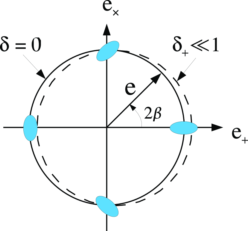
Figure 1: The ring test. In the ring test, objects that have ellipticity magnitude $e=\sqrt{e_{+}^{2}+e_{\times}^{2}}$ are distributed evenly in $\beta$ on a ring in the ellipticity plane (solid circle). In the absence of shear $\delta$, the average of the measured shapes should be zero. In the presence of small shear $\delta_{+}$, the distribution of objects in the ellipticity plane are displaced such that they are no longer arranged with their center on the origin. The average of all the shapes on the displaced ring should behave as Eq. (12), to the first order in $\delta_{+}$.

2.2 Fitting to Basis Functions

The circularity test described in BJ02 involves decomposing the pre-convolution surface brightness distribution of the galaxy, $I(\mbox{\boldmath$\theta$})$, into the Gauss-Laguerre set of orthonormal basis functions in the plane. We consider here a general set of two dimensional functions $\{\psi_{i}(\mbox{\boldmath$\theta$})\}$ that are complete (though not necessarily orthogonal) over the plane. Any set of complete functions can be transformed to a new complete set $\{\psi^{E}_{i}\}$ via

$$\psi_{i}^{E}(\mbox{\boldmath$\theta$})\equiv\psi_{i}({\bf E}^{-1}\mbox{\boldmath$\theta$}).$$ (13)

Here ${\bf E}$ is any remapping of the sky plane that compounds a displacement $\mbox{\boldmath$x$}_{0}$, a shear $\eta$, and a dilation $\mu$. We refer to ${\bf E}$ as the basis ellipse of the function set: if the unit circle is an isophote of $\psi_{i}$, then $\{\mbox{\boldmath$x$}_{0},\mu,\mbox{\boldmath$\eta$}\}$ describe the center, size, and shape of an ellipse that traces the same isophote for $\psi^{E}_{i}$. We will also use ${\bf E}$ to refer to this set of 5 parameters that defines an ellipse; it will be clear from context whether we are referring to the parameter vector or the coordinate transform. For any E we must have

$$I(\mbox{\boldmath$\theta$})=\sum_{i}b_{i}\psi_{i}^{E}(\mbox{\boldmath$\theta$})=\mbox{\boldmath$b$}\cdot\mbox{\boldmath$\psi$}^{E}(\mbox{\boldmath$\theta$}),$$ (14)

for (at least) one vector $b$ of coefficients. For the function set to be complete, the vectors must be infinite-dimensional, but a real measurement will model $I$ with a finite subset of the basis functions. The model must be fit to the observed image plane which we denote with coordinates $x$.

The action of the atmosphere, optics, and detector will operate on $I(\mbox{\boldmath$\theta$})$ to produce an observed surface-brightness distribution $I_{o}(\mbox{\boldmath$x$})$ on the detector plane. This observation operator $C$ likely includes convolution by the PSF and perhaps some distortion by the optics. We will assume that this operation is known and that it is linear over surface brightness, so that $C(aI_{1}+bI_{2})=aC(I_{1})+bC(I_{2})$, where $a$ and $b$ are any two scalars. In this case, Equation (14) must also imply that

$$I_{o}(\mbox{\boldmath$x$}) = \sum_{i}b_{i}\phi_{i}^{E}(\mbox{\boldmath$x$}),$$ (15)

$$\phi^{E}_{i}(\mbox{\boldmath$x$}) \equiv C\left[\psi^{E}_{i}(\mbox{\boldmath$\theta$})\right].$$ (16)

The observed-plane brightness is sampled at the centers of the pixels $\mbox{\boldmath$x$}_{p}$ yielding measurements $I_{p}$ with uncertainties $\sigma_{p}$, assumed henceforth to be Gaussian. The model which maximizes the likelihood of the decompositions (14) and (15), given the data is that which minimizes

$$\chi^{2}=\sum_{p\in\,{\rm pixels}}{\left[I_{p}-\sum_{i}b_{i}\phi_{i}^{E}(\mbox{\boldmath$x$}_{p})\right]^{2}\over\sigma_{p}^{2}}$$ (17)

We call this a “forward fit” to the galaxy image, because we are positing a distribution $\mbox{\boldmath$b$}\cdot\mbox{\boldmath$\psi$}^{E}(\mbox{\boldmath$\theta$})$ of flux on the sky, then propagating this to the detector plane, where we compare the model to the observations. Our task will be to find the ${\bf E}$ for which the $\chi^{2}$-minimizing vector $b$ satisfies the circularity constraints.

For fixed ${\bf E}$, the $\chi^{2}$ minimization is a linear least-squares problem over $b$ with the usual analytic solution

$$b = \mbox{\boldmath$\alpha$}^{-1}\cdot\mbox{\boldmath$\beta$}$$ (18)

$$\beta_{i} \equiv \sum_{p}I_{p}\phi_{i}^{E}(\mbox{\boldmath$x$}_{p})/\sigma_{p}^{2}$$ (19)

$$\alpha_{ij} \equiv \sum_{p}\phi_{i}^{E}(\mbox{\boldmath$x$}_{p})\phi_{j}^{E}(\mbox{\boldmath$x$}_{p})/\sigma_{p}^{2}.$$ (20)

If the $\psi_{i}$ are orthogonal and the noise is stationary and white and the sampling approaches the continuum limit and the PSF approaches a delta-function, then $\alpha$ will be diagonal (modulo some complex conjugation operations) and the solution is very simple. These conditions are not, however, typically met by real data—in particular the sampling and PSF conditions—so it is not safe to use orthogonality to decompose the observed data (BJ, 02; Massey et al., 2004; Berry et al., 2004).

For finite data, the solution must be done over some truncated basis set. We will assume that $N$ of the basis functions are being used, so that $\alpha$, $\beta$, and $b$ have dimension $N$. The $\chi^{2}$-minimizing $b$ is uniquely defined, regardless of whether the $\psi_{i}$ are complete or orthogonal, as long as $\alpha$ is not singular.

To follow the BJ02 prescription we must define circularity tests and iterate the shear in ${\bf E}$ until the two circularity components vanish. At the same time, we may wish to define null tests for the centroid $\mbox{\boldmath$x$}_{0}$ and/or size $\mu$ of the galaxy, so there will be some number $K\leq 5$ such statistics ($K=5$ when there is a null test for each of the parameters of ${\bf E}$). Any test which is linear over the true intensity $I(\mbox{\boldmath$\theta$})$ may be expressed as a linear operation on $b$. Hence the task of the fitter is to adjust $K$ components of the ${\bf E}$ parameters until the $\chi^{2}$-minimizing $b$ satisfies

$${\bf M}\cdot\mbox{\boldmath$b$}={\bf 0}.$$ (21)

${\bf M}$ is a $K\times N$ matrix that defines our tests for matching the basis ellipse to the center, size, and shape of the pre-convolution galaxy.

Once Equation (21) is satisfied for a chosen set of basis functions $\psi_{i}$ and any choice of the circularity-test matrix ${\bf M}$, we obtain a well-defined measurement of the shape $e$ (or more generally the defining ellipse E) of the pre-convolution galaxy image. Since these shapes are defined by shear operations on the $\theta$ plane, they should transform according to Equation (10) and be amenable to all the weighting and responsivity schemes of BJ02.

Before describing how we solve for ${\bf E}$, we summarize the conceptual and practical advantages of combining a transformation-based definition of shape with forward fitting of a pre-convolution model to the observed pixels. Note the fitting approach has been advocated by several authors (Fischer et al., 1997; BJ, 02; Massey et al., 2004; Kuijken, 2006).

• The $e$ values determined in this way transform in a well-known way under lensing shear. The response of a galaxy population to lensing shear can be calculated without recourse to empirical calibration factors beyond the distribution of the $e$ values themselves.

• The forward-fitting procedure can in principle work with any sort of PSF, even those—such as the Airy function—that have divergent second moments.

• The forward-fitting procedure properly handles pixelization and sampling by the detector. Furthermore any aliasing ambiguities will properly propagate into the covariance matrix for $b$, and as described below can be propagated into uncertainties in ${\bf E}$.

• Pixels rendered useless by defects or cosmic rays are easily omitted from the measurement.

• The method is easily extended to simultaneous fitting of multiple images with distinct PSFs. The sum over pixels in Equation (18) is run over all pixels in all exposures of the galaxy. All exposures share the same $b$, $\psi$, and ${\bf E}$ vectors, but have distinct observation operators $C$ and hence different $\phi_{i}$. Information available in the best-seeing images is properly exploited.

• The method is easily adapted to the analysis of $uv$-plane interferometric data rather than image-plane data.

2.3 Iterating the Fit

The desired ellipse parameters ${\bf E}=\{x_{0},y_{0},\mu,\eta_{+},\eta_{\times}\}$ enter the least-squares fit non-linearly, hence some iterative scheme (or Markov chain, cf. Bridle et al. (2002)) is required to determine the values that meet the constraint (21). For a chosen ${\bf E}$, the determination of $b$ has the rapid solution (18). If the current estimate ${\bf E}_{0}$ yields a $\mbox{\boldmath$b$}_{0}$ that does not meet the circularity condition, the Newton-Raphson iteration would be

$${\bf E}_{0}\rightarrow{\bf E}_{0}+\delta{\bf E},\qquad\delta{\bf E}=-\left({\bf M}{d\mbox{\boldmath$b$}\over d{\bf E}}\right)^{-1}({\bf M}\mbox{\boldmath$b$}_{0}).$$ (22)

The derivative $d\mbox{\boldmath$b$}/d{\bf E}$ follows from noting the effect of a small change $\delta{\bf E}$ to the basis of $\psi$:

$$\psi^{E+\delta E}_{i}(\mbox{\boldmath$\theta$}) \approx \psi_{i}^{E}(\delta{\bf E}^{-1}\mbox{\boldmath$\theta$})$$

$$= \psi_{i}^{E}(\mbox{\boldmath$\theta$})+\sum_{k}\delta E_{k}\sum_{j=0}^{\infty}G_{kij}\psi^{E}_{j}(\mbox{\boldmath$\theta$})$$

$$\Rightarrow\phi^{E+\delta E}_{i}(\mbox{\boldmath$x$}) \approx \phi^{E}(\mbox{\boldmath$x$})+\sum_{k}\delta E_{k}\sum_{j=0}^{\infty}G_{kij}\phi^{E}_{j}(\mbox{\boldmath$x$}).$$

Here ${\bf G}_{k}$ is the generator for the transformation indicated by $k$th parameter of ${\bf E}$—either translation, dilation, or shear. These matrices are fixed by the choice of basis functions $\{\psi_{i}\}$. These alterations to the basis-function values can be propagated through the solution (18) to give the perturbation to $b$:

$$\delta\mbox{\boldmath$\beta$} = \sum_{k}\delta E_{k}{\bf G}_{k}\mbox{\boldmath$\hat{\beta}$}$$

$$\delta\mbox{\boldmath$\alpha$} = \sum_{k}\delta E_{k}({\bf G}_{k}\mbox{\boldmath$\hat{\alpha}$}+\mbox{\boldmath$\hat{\alpha}$}^{T}{\bf G}_{k}^{T})$$

$$\Rightarrow\ \mbox{\boldmath$b$}+\delta\mbox{\boldmath$b$} = (\mbox{\boldmath$\alpha$}+\delta\mbox{\boldmath$\alpha$})^{-1}(\mbox{\boldmath$\beta$}+\delta\mbox{\boldmath$\beta$})$$

$$\approx \mbox{\boldmath$\alpha$}^{-1}\mbox{\boldmath$\beta$}+\mbox{\boldmath$\alpha$}^{-1}(\delta\mbox{\boldmath$\beta$})-\mbox{\boldmath$\alpha$}^{-1}(\delta\mbox{\boldmath$\alpha$})\mbox{\boldmath$\alpha$}^{-1}\mbox{\boldmath$\beta$}$$

$$\Rightarrow\quad\delta\mbox{\boldmath$b$} = \sum_{k}\delta E_{k}\left[\mbox{\boldmath$\alpha$}^{-1}{\bf G}_{k}(\mbox{\boldmath$\hat{\beta}$}-\mbox{\boldmath$\hat{\alpha}$}\mbox{\boldmath$b$}_{0})\right.$$ (23)

$$\quad\quad\quad\quad\quad\ \ -\left.\mbox{\boldmath$\alpha$}^{-1}\mbox{\boldmath$\hat{\alpha}$}^{T}{\bf G}_{k}^{T}\mbox{\boldmath$b$}_{0}\right].$$

The matrix $d\mbox{\boldmath$b$}/d{\bf E}$ is apparent from this last equation. Here we have taken the generator matrices ${\bf G}_{k}$ to each be $N\times\infty$; the vector $\hat{\beta}$ now must be, in general, augmented to infinite dimension, and we also take $\hat{\alpha}$ to be $\infty\times N$. Note that the parenthesized portion of the solution (23) would vanish if not for the distinction between the truncated and infinite-dimensional versions of $\alpha$ and $\beta$, since the first $N$ elements of $\mbox{\boldmath$\hat{\beta}$}-\mbox{\boldmath$\hat{\alpha}$}\mbox{\boldmath$b$}_{0}$ are zero. Likewise we could set the initial $\mbox{\boldmath$\alpha$}^{-1}\mbox{\boldmath$\hat{\alpha}$}^{T}$ of the final term to identity if not for the truncation, in which case the transformation would become the very simple $\delta\mbox{\boldmath$b$}=({\bf G}^{T}\mbox{\boldmath$b$}_{0})\cdot\delta{\bf E}$ (with some abuse of notation here). Since we are using $d\mbox{\boldmath$b$}/d{\bf E}$ only to help us iterate the solution for ${\bf E}$, we could use this simple approximation, or extend to some order beyond $N$ using Equation (23).

2.4 The Gauss-Laguerre Decomposition

We use the Gauss-Laguerre decomposition in our shape measurements. These are the eigenfunctions of the 2-dimensional quantum harmonic oscillator, and are most compactly expressed as complex functions indexed by two integers $p,q\geq 0$:

$$\psi_{pq}(r,\theta)={{(-1)^{q}}\over{2\pi}}\sqrt{{q!}\over{p!}}\;r^{m}e^{im\theta}e^{-r^{2}/2}L_{q}^{(m)}(r^{2})\qquad(m=p-q\geq 0).$$ (24)

The elliptical-basis versions are taken to be

$$\psi^{E}_{pq}(\mbox{\boldmath$\theta$})\equiv e^{-2\mu}\psi_{pq}({\bf E}^{-1}\mbox{\boldmath$\theta$}).$$ (25)

Note we have tweaked the normalizations so that the flux is

$$f=\int d^{2}\theta I(\mbox{\boldmath$\theta$})=\sum_{p,q\geq 0}b_{pq}\delta_{pq}$$ (26)

rather than making the functions orthonormal. The Gauss-Laguerre (GL) functions are still, however, a complete and orthogonal set over the plane. The functions are equivalent to the “polar shapelets” of Massey et al. (2004).

The advantages of the GL functions as our basis are:

• The $\psi_{i}$ are rapidly calculable via recursion relations.

• Decompositions of typical ground-based PSFs and exponential-disk galaxies are reasonably compact.

• There are obvious choices for the circularity tests: the centroiding condition is $b_{10}=0$; the circularity condition is $b_{20}=0$; and a size-matching condition is $b_{11}=0$. The matrix ${\bf M}$ is very simple, i.e. it just restricts $b$ to five relevant (real-valued) elements.

• The generator matrices ${\bf G}_{k}$ are sparse and simple. In particular, if the truncated $b$ extends to $p+q\leq N$, then ${\bf G}_{(pq)(p^{\prime}q^{\prime})}$ vanishes for $p^{\prime}+q^{\prime}>N+2$. This means that the augmented $\hat{\alpha}$ and $\hat{\beta}$ in Equation (23) can be calculated exactly simply by extending the sums in Equation (18) to order $N+2$ (in $p+q$), just slightly beyond the order $N$ needed to calculate $b$.

• Matrices for finite transformations are calculable with fast recursion relations.

• Convolution by a PSF is also expressible as a matrix operation over the $b$ vector, if we also express the PSF as a GL decomposition $\mbox{\boldmath$b$}^{\star}$ in some basis ellipse ${\bf E}^{\star}$. This means that the $\phi_{i}$ corresponding to a chosen PSF are rapidly calculable.

BJ02 contains details on many of these properties, and gives the generators (§6.3.2), the forms for the finite-transformation matrices (Appendix A), and the convolution matrices (Appendix B). We emphasize that other basis sets may be chosen which yield valid shape measurements, but we choose the GL decomposition for its efficiency and clarity. Similarly, one need not execute the operation $C(\psi_{pq})$ using the GL matrices; this is just a computational convenience in our case.

2.5 Alternative Circularity Tests

We follow BJ02 in using $b_{20}=0$ as our definition of a circular object. It is possible that other GL coefficients carry shape information that could be used to produce lower-noise shape estimates (Massey et al., 2004). In fact with the formalism used below (§2.6) to estimate shape uncertainties, one can derive for each object a linear circularity test $M$ that is optimally sensitive to shear. We have implemented a scheme whereby such an optimally weighted combination of all the quadrupole coefficients $(m=p-q=\pm 2)$ is derived for each galaxy. Our testing has not yet demonstrated any significant advantage to this scheme, however, so we have not pursued it further for fear that such custom estimators might produce subtle noise-rectification biases.

2.6 Error Estimates

We may produce uncertainties on the ellipse parameters $E_{k}$ by propagating the pixel flux uncertainties. The covariance matrix for the $b$ vector takes the usual form ${\bf C}^{b}=\alpha^{-1}$. The covariance matrix for the ellipse parameters then follows:

$${\bf C}^{E}=\left({d\mbox{\boldmath$b$}\over d{\bf E}}\right)^{-1}{\bf C}^{b}\left[\left({d\mbox{\boldmath$b$}\over d{\bf E}}\right)^{-1}\right]^{T}$$ (27)

We may also assign a detection significance to the object. In the simplest case, where there is no PSF to consider, the signal-to-noise ratio $S/N$ for detection by the optimally-sized elliptical Gaussian filter is given by

$$\nu^{2}={b_{00}^{2}\over{\rm Var}(b_{00})}.$$ (28)

The maximization of this quantity with respect to the size, shape, and center of the elliptical-Gaussian filter generates conditions that are identical to our default circularity tests.

We define a significance in the more general case—such as when the PSF is non-trivial—to be

$$\nu^{2}={f^{2}\over{\rm Var}(f)},\qquad f=\sum_{p}b_{pp}.$$ (29)

The variance on the flux can be obtained by contracting ${\bf C}^{b}$. This estimate of the significance corresponds to the signal-to-noise on the galaxy detection that would be obtained by applying a filter to the deconvolved image that is matched to the shape, location, and radial profile of the galaxy. The maximum order of the sum in (29) determines the allowable complexity of the filter.

3 Description of GLFit

GLFit is the C++ implementation of the methods described in the previous section. The code includes classes to represent the vectors, transformations, and covariance matrices over quantities indexed by the integer pairs $pq$. To fit to a single galaxy, the code requires as input:

• Image-format data for both the surface brightness $I_{p}$ and the weight $1/\sigma^{2}_{p}$ (cf. Eq. (17)). The latter image should be set to zero at saturated, defective, or contaminated pixels. Data/weight image pairs from multiple exposures may be submitted for simultaneous fitting of a single object. It is assumed that each image has been flat-fielded so that a source of uniform surface brightness has equal value in all pixels.

• For each exposure, a map $\mbox{\boldmath$\theta$}(\mbox{\boldmath$x$})$ from the pixel coordinate system into the world coordinate system. This is typically either the distortion map into the local tangent plane to the celestial sphere, or an identity map.

• For each exposure, the local sky brightness and a photometric gain factor.

• If we are executing a deconvolution fit, whereby we measure the shape of the galaxy before PSF convolution, then we require, for each exposure, a vector $\mbox{\boldmath$b$}^{\star}$ and basis ellipse ${\bf E}^{\star}$ describing the estimated PSF at the location of the galaxy. If we are executing a native fit, whereby we are trying to measure the observed shape of the galaxy, then no PSF information is required.

• A choice for the initial order $N$ $(p+q\leq N)$ of the GL decomposition of the galaxy model.

• Lastly an initial estimate of the size, location, and shape of the galaxy, e.g. the values generated by detection software such as SExtractor (Bertin & Arnouts, 1996). If we are executing a deconvolution fit, we need to know both the size $\sigma_{o}=e^{\mu_{o}}$ of the object as observed, and the size $\sigma_{\star}$ of the PSF in which the object is observed. These are by default subtracted in quadrature to estimate the size $\sigma_{i}$ of the intrinsic (pre-seeing) galaxy.

The procedure for shape determination has the following steps:

1. If we are executing a deconvolution fit, we choose the size of the “source basis” ${\bf E}_{s}$ which is the basis ellipse for the $\psi^{E}_{i}$ that will be used to model the pre-convolution image. We select

   $$e^{2\mu_{s}}=\sigma^{2}_{s}=\sigma^{2}_{i}+f_{\rm PSF}\sigma^{2}_{\star},$$ (30)

   where $\sigma^{2}_{i}$ and $\sigma^{2}_{\star}$ are the sizes of the pre-seeing galaxy image and the PSF, respectively, and $f_{\rm PSF}$ is a prefactor chosen by default to be 1.2. If there are multiple exposures, we take $\sigma_{\star}$ to be the harmonic mean of all the exposures’ PSF sizes. As discussed in BJ02 §6.2, we expect a choice of Gaussian basis $\sigma$ that is larger than both the intrinsic galaxy and the PSF to offer the most sensitive measure of pre-convolution quadrupole moments. During a deconvolution fit, $\mu_{s}$ is held fixed during all iterations and there is no constraint on size in the circularity test ${\bf M}$.

2. The initial guess for ${\bf E}_{s}$ is mapped from the world coordinate system into each exposure’s pixel system. An elliptical mask is created for each exposure, defined by the $n\sigma$ contour of the elliptical Gaussian. Typically we select $n\approx 4$. Pixels outside the mask are not included in the fit. Larger masks reduce the possibility of degeneracy or non-positive models for high-order fits, but increase the chance of contamination by neighboring objects.

3. If any of the exposures do not fully contain the fitting mask, the Edge flag is set. If the initial centroid falls outside all the exposures, then the OutOfBounds flag is set and the fit is terminated.

4. The basis ellipse ${\bf E}^{\star}$ of the PSF is changed to have the same shape (not size) as the current estimate of the galaxy shape, by applying a finite shear transformation matrix to $\mbox{\boldmath$b$}^{\star}$. The convolution by the PSF is now expressed as a matrix operation, so we have an observed-plane image model

   $$I_{o}(\mbox{\boldmath$x$})=\sum_{i,j}\psi^{E_{o}}_{i}[\mbox{\boldmath$\theta$}(\mbox{\boldmath$x$})]C_{ij}b_{j}.$$ (31)

   The observed-plane basis ellipse ${\bf E}_{o}$ has second moments that are the sum of the second moments of the chosen source-plane basis ${\bf E}_{s}$ and the PSF basis ellipse. The convolution matrix elements $C_{ij}$ can be computed as in Appendix B of BJ02. We now have a model for the observed data which is linear over the expansion coefficients $b$.

5. The linear solution for $b$ is executed by summing over all valid pixels within the masks on all exposures. If a singular value decomposition of the $\alpha$ matrix indicates that there are poorly constrained combinations of $b$ elements, the order of the GL decomposition is reduced by one (to a minimum of $N=2$), the ReducedOrder flag is set, and the solution is attempted again.

6. The matrix $d\mbox{\boldmath$b$}/d{\bf E}$ is calculated from the augmented $\hat{\alpha}$ and $\hat{\beta}$ (which in fact were calculated in the previous step) as per Equation (23).

7. If the circularity test applied to $b$ is not zero within a specified tolerance, then an iteration increment $\delta{\bf E}$ is calculated according to Equation (22). If a singular-value decomposition of $d\mbox{\boldmath$b$}/d{\bf E}$ indicates a nearly-degenerate matrix, we know that there is no sensible estimate for the next step. In other words, at least one of our circularity tests is currently ill-defined, for example no small change of basis makes the object appear more circular. This should, for example, be the case for a point source, but also arises for some very irregular or noisy galaxies. The behavior of the next step depends upon the fit type: In a native fit, we set the FrozeDilation flag, set $\mu$ back to its initial value, and restart the fitting process, this time holding $\mu$ fixed. If we are executing a deconvolution fit, we increment $f_{\rm PSF}$ by 0.5, set the RaisedMu flag, and restart the fitting process, since fits to a larger basis tend to be more stable (but less sensitive). If FrozeDilation has been set (for a native fit) or $f_{\rm PSF}>3$ already (for a deconvolution fit), and $d\mbox{\boldmath$b$}/d{\bf E}$ is still near-degenerate, then our last resort is to set the FrozeShear flag, reset $\eta$ to its starting value, and restart the fit process while holding the shape fixed.

8. The next iteration of the fitting process continues at step 31. If the circularity test is not satisfied within a chosen number of iterations, the DidNotConverge flag is set and the fit is terminated. If any other matrix singularities are encountered, or if there are too few pixels to conduct the fit, the Singularity flag is set, and the fit terminates.

9. Once the circularity tests are satisfied within a desired tolerance, the resultant ${\bf E}$ and $b$ for the galaxy are available for the user. The $\alpha$ matrix provides the covariance matrix for $b$. The errors on the centroid, size, and ellipticity (or whichever of these were free to vary) are calculated using Equation (27), and a detection significance can be reported using Equation (29).

In most cases the solution for ${\bf E}$ is executed twice: first, a coarse fit at order $N=2$ is attempted. If this fails, the CoarseFailure flag is set. If it succeeds, the coarse solution is used as the starting point for a fit to the full requested $N$.

Another subtlety is that the pixel mask is not changed between iterations—the mask maintains the shape and size specified by the initial guess (or the result of the coarse fit). This should not bias the fit toward the initial guess, however, because we are fitting to the data within the mask rather than executing a sum of moments over pixels within the mask. If the size $\mu$ of the object changes dramatically during the coarse fit (e.g. due to a very poor initial estimate from SExtractor), then we do resize the masks and start over. If at any time the mask on an image grows to encompass too large a number of pixels, we set the TooLarge flag and quit. This prevents the program from getting hung up calculating pixel sums for nonsensically large objects.

The algorithm is considered to have converged to a valid shape measurement if it completes without setting of the flags FrozeShear, DidNotConverge, Singularity, OutOfBounds, TooLarge, or CoarseFailure.

4 Test Procedure

In our tests, postage-stamp images are created of individual galaxies, as convolved with a known PSF, pixelized, and given noise. We then extract shape and shear measurements from ensembles of such postage-stamp tests. In the real sky and in end-to-end tests which draw (pre-lensing) galaxy shapes at random, the uncertainties in the output shear are usually dominated by the finite variance of the mean pre-shearing shape (shape noise). We construct our ensembles with zero mean shape to eliminate shape noise, leaving our testing precision dominated by the shot noise in the images.

Because we provide the shape-measurement algorithms with an approximate location for every simulated galaxy, our tests do not include the effects of possible selection biases (Kaiser, 2000; BJ, 02; HS, 03). Similarly the PSF is always presumed to be known exactly, so we do not test for errors that would result from PSF measurement or interpolation errors (van Waerbeke et al., 2005; Jain et al., 2006). Effects of galaxy crowding or overlap, detector nonlinearities, intrinsic galaxy-shape correlations, or redshift determination errors (Ma et al., 2006) are not examined here. Instead we concentrate on the sources of systematic error that arise specifically from (1) the shape measurement, (2) removal of the PSF effects, and (3) the shear estimation, in images with finite noise and sampling.

4.1 Test Conditions

In order to test our WL analysis methodology, we need to find the conditions under which GLFit works, and then test for any biasing in the shape measurement or shear estimation method. The following is the list of the test conditions or choices made:

• Native fit or deconvolution fit. All measurements are tested for cases without (native fit) and with (deconvolution fit) the presence of a PSF. In a WL analysis of real sky data, native fits are used in (1) characterizing the PSF from stellar images, and (2) measuring the shape of the PSF-smeared galaxy, whose value is used to produce an initial estimate of the intrinsic galaxy shape.

• Galaxy size with respect to pixel or PSF. As the pixel sampling rate decreases, it becomes harder to obtain shape information about the galaxy from the pixelized image, or for the GLFit to converge. For the native fits, the galaxy size is defined with respect to the pixel; for the deconvolution fits, to the PSF.

• Galaxy detection significance $\nu$, or equivalently $S/N$. If the background noise dominates the signal from the galaxy, GLFit is also unlikely to converge.

• Galaxy shape $e$. The galaxies are sheared to various shapes, ranging from $|e|=0$ to $0.9$ ($=$ axis ratio $4.35:1$). In some cases, the major axis orientation (parallel or diagonal to the pixel axis) is also examined.

• Galaxy type. We choose a “symmetric” or “asymmetric” galaxy model, with the latter being a more stringent test of the methodology. The galaxy models are described further in §4.2, and the shear accuracy is examined by the ring test, described in §4.3.

For the deconvolution fit, we have the following additional choices for the PSF:

• PSF type. We choose an Airy disk PSF as the worst possible case for a PSF. An Airy disk offers particular difficulties for shape-measurement algorithms, such as its non-trivial morphology and divergent second moments.

• PSF shape. The Airy disk is either circular or elliptical (sheared at $e_{\rm PSF}=0.1$). We look for any leakage of the PSF shape into the galaxy shape measurement or the shear estimate.

In this paper, the PSF is always known; we do not test for errors due to incomplete knowledge of the PSF.

4.2 Pixelized Galaxy Models

Two types of galaxies, symmetric and asymmetric, are used to test the shape measurement and shear recovery. The galaxy models, along with any shear, rotation, and dilation, are described as an analytic function over the pixel coordinates.

The “symmetric” galaxies have either a Gaussian or exponential circularly symmetric radial profile that is then sheared. All isophotes are similar ellipses, so these galaxies have unambiguous shapes, which allows direct comparison between the input and measured shape. The elliptical symmetry of these galaxies could be masking errors in the shape-measurement methodology by causing fortuitous cancellations of errors. In other words, all of their EGL expansion coefficients with $m\neq 0$ are exactly zero, so any biases that couple to these coefficients will not be tested by the symmetric galaxies.

The “asymmetric” galaxies are designed so that they have no inversion symmetry, and their isophotal shape varies with radius; i.e., there is no unambiguously defined shape. The ring test is therefore needed to see if input shear is accurately recovered. These are constructed as a combination of exponential and deVaucouleur ellipses, each with different flux, size, and shape, as well as a slight offset between the two centroids. The asymmetric galaxies offer a more stringent test of shear measurement, since we have broken any symmetries that could mask errors in the shape measurement.

A pixelized postage stamp image is created from the analytic functions that describe the galaxy and PSF models at the intended sampling rate. The centroid of the analytic functions is randomized within the pixel over multiple image realizations (pixel phase randomization). The PSF convolution is done either analytically if possible, or via FFT of noiseless pixelized images. The Poisson photon noise is then added to produce the final image to produce the desired $S/N$ for the object. We then run GLFit for shape measurement with starting parameters randomly displaced from the true values.

4.3 The Ring Test

The ring test evaluates the mean shape—the weighted average of the galaxy shape components—with a simplified galaxy shape distribution, as seen in Figure 1. When a shear $\delta$ is uniformly applied to the ensemble, the mean shape $\langle\mbox{\boldmath$e$}\rangle$ should equal ${\mathcal{R}}\mbox{\boldmath$\delta$}$, where ${\mathcal{R}}=1-\frac{e^{2}}{2}$ (Eq. (12)) is called the responsivity. This relation then gives an estimate of the shear from the mean shape.

The value of the ring test is two-fold: the expected signal is known, and the shape noise is absent. The shape noise in WL is the statistical noise due to the random distribution of shapes with finite magnitudes; the uniform distribution of shapes in the ring test eliminates this noise. The lack of shape noise and the known expected value then allow systematic errors to be quantified.

5 Results

5.1 GLFit Convergence

We run GLFit on objects with different size and detection significance to understand the conditions under which GLFit converges reliably, which we define to be $>99\%$ rate of successful shape measurement. Shear estimate accuracy tests are subsequently performed only in $>99\%$ convergence conditions, to preclude any selection biases that could be generated by the non-convergence of GLFit.

5.1.1 Native Fit Convergence

Figure 2 shows the $99\%$ convergence contour for native fits on exponential-profile symmetric galaxies of various ellipticities. The upper right hand region delineated by the contour indicates where the fit has $>99\%$ convergence. The horizontal axis indicates the sampling rate, and is expressed in terms of the “minor axis width” (MAW), defined below. The vertical axis incidates the detection significance $\nu$ of the object.

We define the minor axis width for a Gaussian object as its full width at half maximum (FWHM) along the minor axis direction. For non-Gaussian objects, the “Gaussian size” $\sigma$ is defined from the size-matching condition $b_{1\!1}=0$ (§2.4); an exponential profile $I(r)=I_{0}\exp(-r/r_{0})$ has a Gaussian size $\sigma\simeq 1.16r_{0}$. The Gaussian size along the minor axis is $\sigma_{b}=\sigma\exp(-\eta/2)$, where $\eta$ is the conformal shear (§2.1), so the minor axis width is $2.35\sigma_{b}$.

Figure 2(a) clearly shows that for a native fit to converge reliably, $S/N$ must be $\geq 10$ and its minor axis width be $\geq 2.8$ pixels. The convergence contour for Gaussian radial profiles is found to be identical to the exponential-profile contour. The fact that the minor axis dimension is the limiting factor for convergence implies a shear-dependent selection, since $\sigma_{b}$ does not remain constant under a shear operation.

The required sampling rate depends, however, on the orientation of the minor axis. Figure 2(a) shows the convergence contour when the ellipse is elongated along the pixel axis, where Figure 2(b) shows the case when the elongation is along the pixel diagonal. In the second case, the required sampling rate appears to decrease with increasing $e$, until it settles at 2.0 pixel for $e\geq 0.6$. Figure 3 illustrates that for objects elongated along the pixel diagonal, the effective sampling rate along the minor axis becomes $1/\sqrt{2}$ of the pixel spacing.

The GL decomposition of the PSF is determined via a native fit. Hence, the images must sample the PSF minor axis width by more than 2.8 pixels for the GLFit to be applied successfully to individual stars. Note that it is possible to increase the sampling rate by dithering for a CCD of any pixel size.

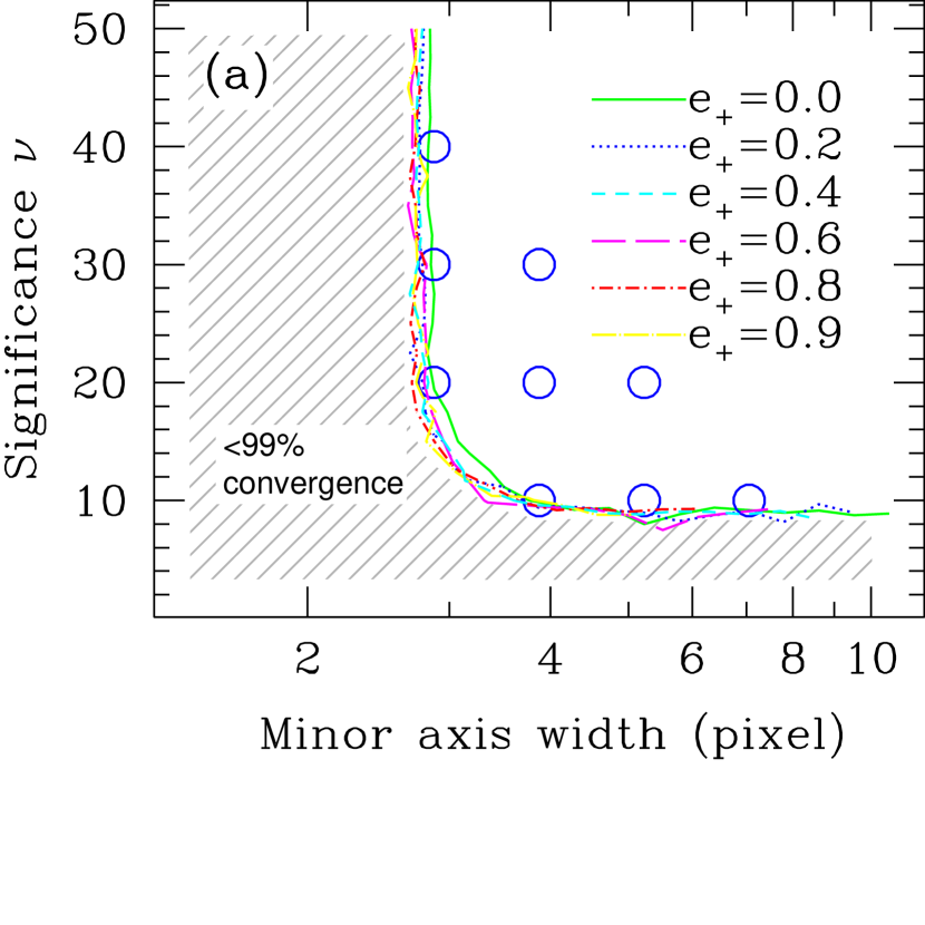
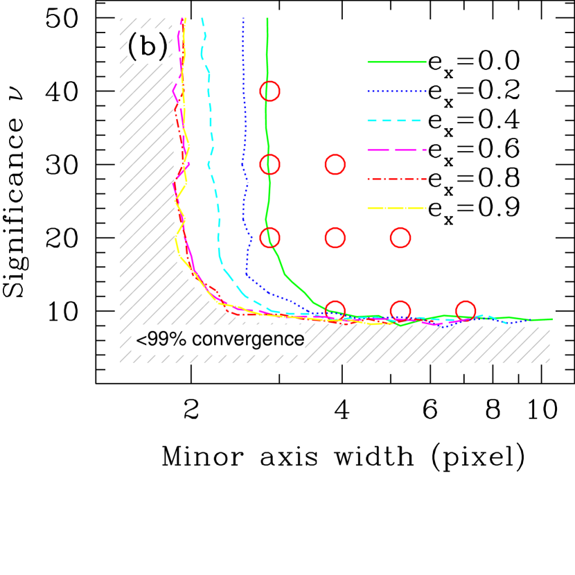
Figure 2: Contours of 99% successful GLFit native-fit convergence over pixel sampling (horizontal axis) and object $S/N$ (vertical axis). The pixel sampling is defined as the FWHM along the minor axis direction, or the “minor axis width”. The shaded region is where the native-fit convergence rate is $<99\%$. (a) Convergence when major axis is along the pixel axis. (b) Convergence when major axis is along the pixel diagonal. The shift in the contour in (b) is due to an effectively new pixel spacing (cf. Fig. 3). The circles in each plot indicate the parameters at which the shape measurement accuracy tests have been performed (cf. Fig. 5).

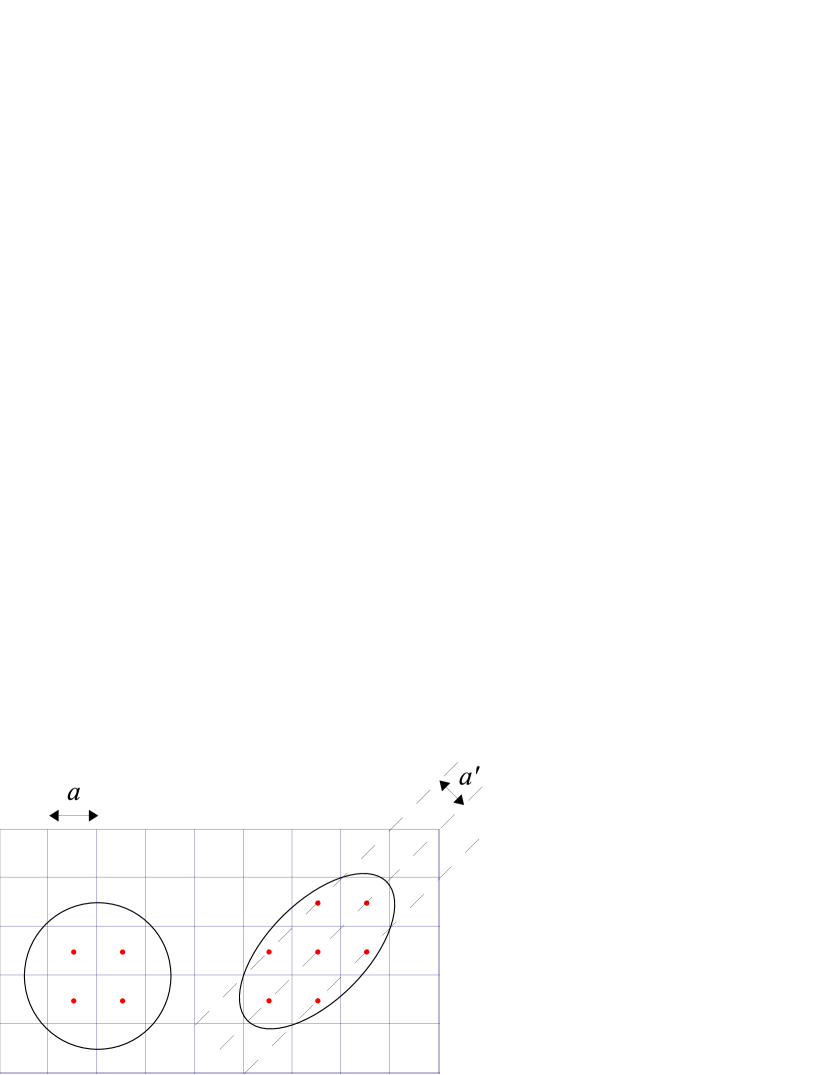
Figure 3: Relation of the minimum measureable object size (Fig. 2) to the pixel lattice for native GLFit. The circle and the ellipse have the minimum minor-axis width for reliable shape measurement in native fits. For the ellipse on the right ($e_{\times}=0.6$), the sampling spacing along the minor axis, $a^{\prime}$, is effectively $1/\sqrt{2}$ of the pixel lattice spacing $a$. The sampling spacing is still $a$ for ellipses stretched along the pixel axis. We note that the the object center is placed at random locations within the pixel in our simulations.

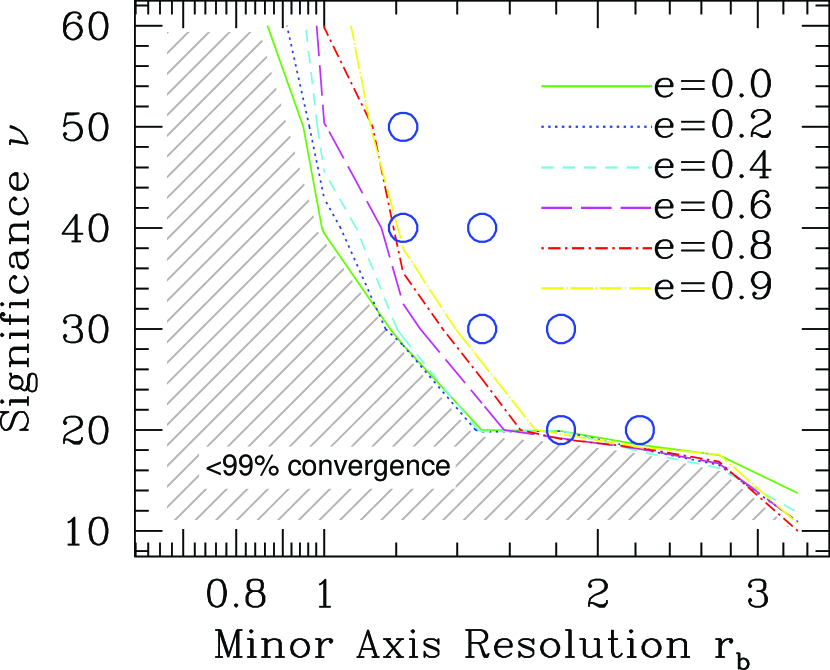
Figure 4: Contour for 99% deconvolution-fit shape measurement convergence over resolution (horizontal axis) and object $S/N$ (vertical axis), for an Airy PSF convolution. The shaded region is where the deconvolution-fit convergence rate is $<99\%$. The resolution is expressed as $r_{b}\equiv\sigma_{b}/\sigma_{\rm PSF}$, where $\sigma_{\rm PSF}$ and $\sigma_{b}$ are the characteristic Gaussian widths for the PSF and along the galaxy minor axis, respectively. The contour is independent of the orientation of the major axis. The circles indicate the parameters at which the shape measurement accuracy tests have been performed (cf. Fig. 8).

5.1.2 Deconvolution Fit Convergence

For the deconvolution test, we convolve the model galaxies with a circular Airy-function PSF, whose characteristic width is $\sigma_{\rm PSF}\simeq 0.21\,\lambda/D$. The model galaxies in this test are symmetric elliptical objects of exponential radial profile with minor axis Gaussian width $\sigma_{b}$ before PSF convolution. The pixel size is irrelevant to the convergence rate, as long as $\sigma_{\rm PSF}\geq\,2.8$ pixels (cf. §5.1.1). We find that the convergence rate of GLFit is independent of the orientation of the major axis under these conditions.

Figure 4 shows the 99% convergence contour for deconvolution fits. The horizontal axis is the minor-axis resolution

$$r_{b}\equiv\sigma_{b}/\sigma_{\rm PSF}.$$ (32)

We find that high-$e$ galaxies are less likely to converge at low resolution than more circular galaxies.

In analyses of the real sky, the dimmest and smallest galaxies are most numerous, so we draw our attention to the lower left corner of the contour in Figure 4. GLFit will converge reliably for objects with $r_{b}\geq\,1.8$ down to $\nu\geq 20$. To obtain a reliable shape measurement of marginally resolved objects ($r_{b}\geq 1.2$) at all shapes $e$, the significance must be $\nu\geq 40$.

5.2 Accuracy for Symmetric Galaxies

Having determined where GLFit is consistently successful in measuring a shape, we now examine the accuracy of the shape measurement and error estimate that result.

When an elliptical object is used as an input, the input shape is well defined, and hence so is the measurement error. In this section we use symmetric elliptical galaxies with exponential radial profile that have an unambiguous shape $\eta_{\rm input}$. The shape measurement error is expressed as a conformal shear $\Delta\eta\equiv(-\eta_{\rm input})\oplus\eta_{\rm meas}$, where $\oplus$ is the shear addition operator, equivalent to shear matrix multiplication:

$$\mbox{\boldmath$\eta$}_{3}=\mbox{\boldmath$\eta$}_{2}\oplus\mbox{\boldmath$\eta$}_{1}\ \ \ \ \Leftrightarrow\ \ \ \ {\bf S}_{\mbox{\boldmath$\eta$}_{3}}{\bf R}={\bf S}_{\mbox{\boldmath$\eta$}_{2}}{\bf S}_{\mbox{\boldmath$\eta$}_{1}},$$ (33)

where ${\bf R}$ is the unique rotation matrix that allows ${\bf S}_{\mbox{\boldmath$\eta$}_{3}}$ to be symmetric (BJ02 §2.2). The quantity $\Delta\eta$ is the amount of shear required to bring the input shape to the measured shape, hence describes a shear bias regardless of the intrinsic object shape. Each data point is an average over $N=100,000$ measurements of independent realizations of pixel phase and photon noise. We then plot the averaged error components $\langle\Delta\eta_{+}\rangle$ or $\langle\Delta\eta_{\times}\rangle$ as the measurement accuracy. The uncertainty in the mean $+$ component is then $\sigma_{\langle\eta_{+}\rangle}=\sqrt{\sum(\Delta\eta_{+})^{2}/N^{2}}$.

GLFit produces error estimates $\tilde{\sigma}_{\eta_{+}}$, $\tilde{\sigma}_{\eta_{\times}}$ for every shape measurement from the covariance matrix ${\bf C}^{E}$ (§2.6). We test for the accuracy of this estimation by examining the averaged ratios $\langle(\Delta\eta_{+})^{2}/\tilde{\sigma}^{2}_{\eta_{+}}\rangle$ and $\langle(\Delta\eta_{\times})^{2}/\tilde{\sigma}^{2}_{\eta_{\times}}\rangle$, where the average is over shape measurement trials.

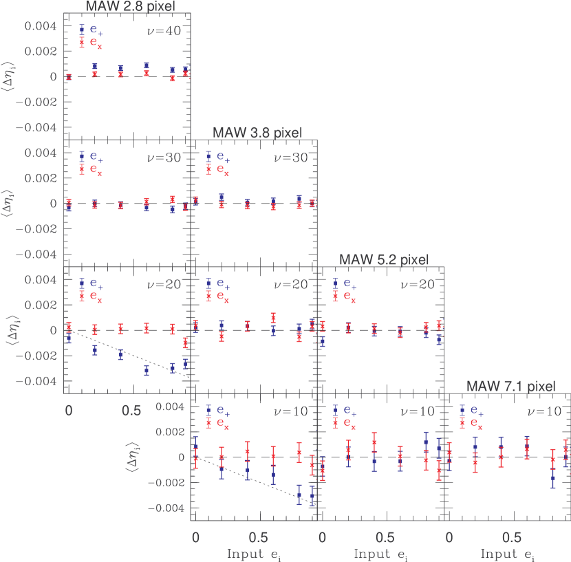
Figure 5: The error in native fit shape measurement as a function of the input shape $e$. The “shape error” $\Delta\eta$ is the amount of shear necessary to bring the measured shape to the input shape; $\Delta\eta_{i}$ is the $i$th component of the error. The plots in the same column have the same minor axis width (MAW$\equiv 2.35\sigma_{b}$), whereas the plots in the same row have the same significance $\nu$; each panel correspond to the set of $(\nu,{\rm MAW})$ parameters indicated by the circles in Figs. 2(a) and (b). The slanted, dotted line in two of the panels indicate shape error of $\Delta\eta_{i}/e_{i}=-0.4\%$, where $i=+,\times$.

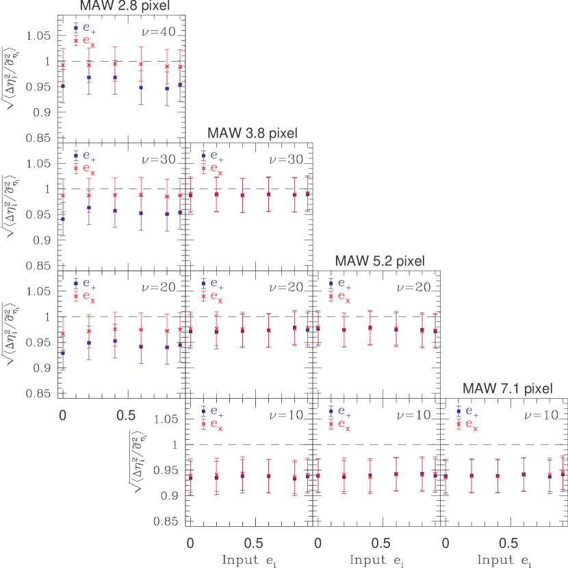
Figure 6: The RMS average of the ratio of measured error to estimated error. The error estimate $\tilde{\sigma}_{\eta_{i}}$ is obtained from the fitting process (cf. §2.6). Each panel correspond to the set of parameters indicated by the circles in Figs. 2(a) and (b).

5.2.1 Native Fit Errors

Each panel in Figure 5 show the average error $\langle\Delta\eta_{i}\rangle$ ($i=+,\times$) as a function of the input shape $e$ of the symmetric exponential galaxies. We first examine the accuracy of native fits to galaxies with no PSF convolution. The panels correspond the sampling rates and detection significances marked by the points inside the 99% convergence contour in Figure 2.

Those that are well into the $>99\%$ convergence region (the inner three panels) show no systematic bias in the shape measurement within the uncertainty $\sigma_{\langle\eta_{i}\rangle}\raisebox{-3.44444pt}{$\stackrel{{\scriptstyle\textstyle<}}{{\sim}}$}\,0.0005$. For those on the $99\%$ convergence contour (left-most and bottom panels), shape measurements show some systematic errors, but the worst systematic is still within $\Delta\eta_{i}/e_{i}\simeq 0.4\%$. The shear error $\Delta\gamma/\gamma$ ($=m-1$ if $c=0$) that would result from such measurement error is

$$\frac{\Delta\gamma}{\gamma}\ \simeq\ f\frac{\Delta\eta_{i}}{e_{i}},$$ (34)

assuming $\Delta\delta/\delta\simeq\Delta\gamma/\gamma$, where

$$f\simeq\left[\frac{1+\langle e^{2}\rangle/2}{1-\langle e^{2}\rangle/2}\right](1-\langle e^{2}\rangle)$$ (35)

for a constant $\Delta\eta_{i}/e_{i}$. The function $f$ is always $<1$, and rapidly decreases to zero for $0.6\,\raisebox{-3.44444pt}{$\stackrel{{\scriptstyle\textstyle<}}{{\sim}}$}\,e<1$. Hence a shape measurement systematic of $\Delta\eta_{i}/e_{i}\simeq 0.4\%$ approximately corresponds to a shear calibration error of $\Delta\gamma/\gamma\simeq 0.4\%$.

Figure 6 shows the root-mean-square (RMS) of the actual to estimated error ratios, $\sqrt{\langle\Delta\eta_{i}^{2}/\tilde{\sigma}_{\eta_{i}}^{2}\rangle}$, where $\tilde{\sigma}_{\eta_{i}}$ is the error estimate in the $i$th component as calculated by GLFit. Overall, we see that the error estimate does fairly well. There is a slight tendency to overestimate the error as $\nu$ becomes low; the $\tilde{\sigma}_{\eta_{i}}$ bias has no dependence on the pixel sampling. The $\nu$ dependence is approximately $\sqrt{\langle\Delta\eta_{i}^{2}/\tilde{\sigma}_{\eta_{i}}^{2}\rangle}\simeq$ $1-\frac{0.6}{\nu}$.

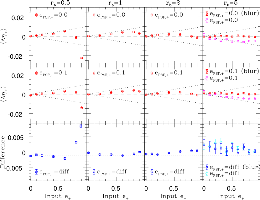
Figure 7: The error in deconvolution shape measurement at $\nu=100$, at resolutions $r_{b}=0.5$, $1$, $2$, and $5$. The plots in the same column have the same resolution. The top row is convolved with a circular Airy PSF; middle row with an elliptical Airy PSF ($e_{\rm PSF}=0.1$); the bottom row is the difference between the two. In the top two rows, the slanted, dotted lines indicate shape error of $\Delta\eta_{+}/e_{+}=\pm 1\%$, where in the bottom row, the dotted lines indicate $\langle\Delta\eta_{+}\rangle=\pm 0.001$, or $1\%$ of the PSF anisotropy. For $r_{b}=5$, the systematic specifically due to the GL decomposition of the Airy PSF is removed by intentionally blurring both the PSF and the observed image with a Gaussian that is a fraction of the size of the galaxy.

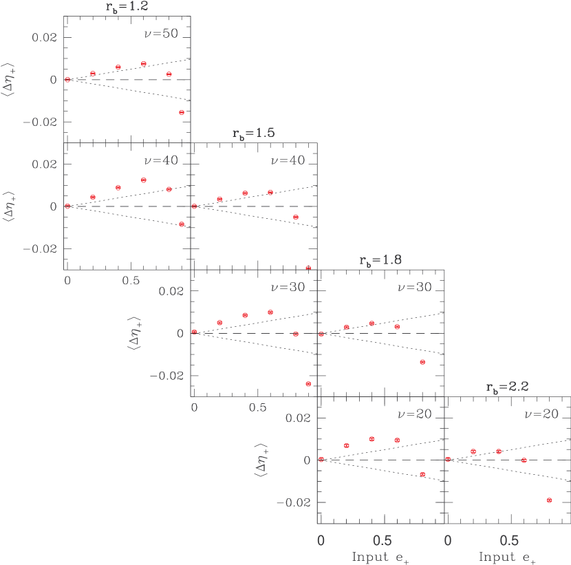
Figure 8: The error in deconvolution shape measurement for $\nu\leq 50$. The Airy PSFs are isotropic ($e_{\rm PSF}=0$). The plots in the same column have the same resolution $r_{b}$, whereas the plots in the same row have the same significance $\nu$; each panel correspond to the set of $(\nu,r_{b})$ parameters indicated by the circles in Fig. 4. These plots are similar to those on the top row of Fig. 7. The slanted, dotted lines indicate shape error of $\Delta\eta_{+}/e_{+}=\pm 1\%$.

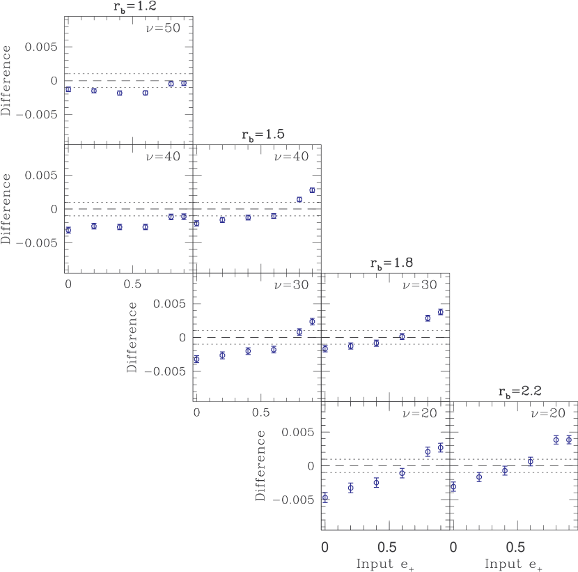
Figure 9: The PSF anisotropy bias in deconvolution shape measurement for $\nu\leq 50$. Each panel correspond to the set of $(\nu,r_{b})$ parameters indicated by the circles in Fig. 4. These plots are similar to those on the bottom row of Fig. 7. The dotted lines indicate $\langle\Delta\eta_{+}\rangle=\pm 0.001$, or $1\%$ of the PSF anisotropy.

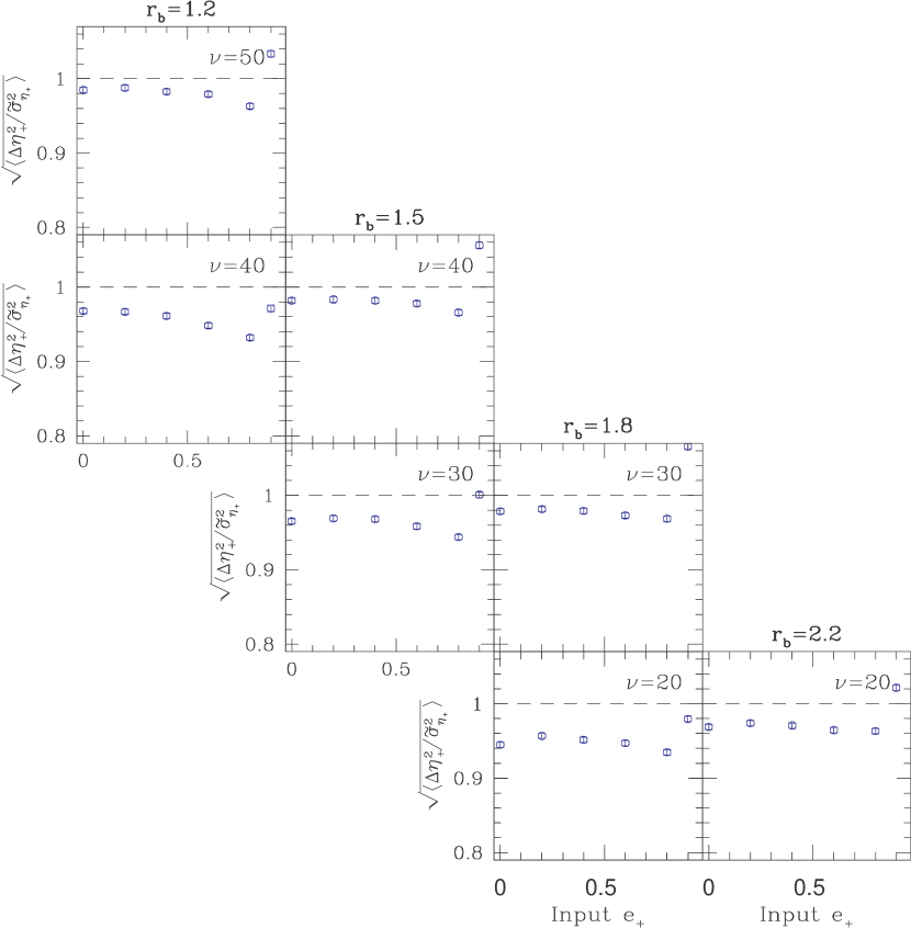
Figure 10: The RMS ratio of actual ($\Delta\eta_{+}$) to estimated ($\tilde{\sigma}_{\eta_{+}}$) errors for deconvolution fits. Each panel correspond to the set of $(\nu,r_{b})$ parameters indicated by the circles in Fig. 4.

5.2.2 Deconvolution Fit Errors

Figure 7 shows the accuracy of a deconvolution fit when a symmetric, exponential galaxy is convolved with an Airy PSF. We first discuss a high-$S/N$ case, $\nu=100$. The measurements were done at various minor axis resolutions, where $r_{b}=0.5$, 1, 2, and 5 each correspond to the columns from left to right.

The panels in the top two rows show the shape error $\langle\Delta\eta_{i}\rangle$ as a function of the input galaxy ellipticity. In the top row, the Airy PSF is circular ($e_{\rm PSF}=0.0$), while in the middle row the Airy PSF is anisotropic, with an ellipticity of $e_{\rm PSF}=0.1$. The PSF and galaxy ellipticity both are elongated along $e_{+}$; we find that the results do not change even if we add a non-zero $e_{\times}<0.15$ component to either the PSF or the galaxy. The major axis orientation with respect to the pixel axis is irrelevant for deconvolution fits (cf. §5.1.2).

The bottom row plots the difference in average measured shape between $e_{\rm PSF}=0.1$ and $e_{\rm PSF}=0.0$. If the PSF anisotropy is fully suppressed in the deconvolved galaxy-shape measurement, this difference should be zero.

In general, Figure 7 shows the following two systematic shape measurement errors: (1) Regardless of the PSF anisotropy, the measurement error exhibit a slight systematic when the resolution is low ($r_{b}<2$). There is a constant positive slope in $\langle\Delta\eta_{+}\rangle$ between $0<e<0.6$. (2) For $e>0.6$, the slope turns around, eventually underestimating the shear at $e=0.9$. In the region described by (1), the shear measurement errors are approximately $\langle\Delta\eta_{i}\rangle\,\raisebox{-3.44444pt}{$\stackrel{{\scriptstyle\textstyle<}}{{\sim}}$}\,0.01e_{i}$, corresponding to $\Delta\gamma/\gamma\,\raisebox{-3.44444pt}{$\stackrel{{\scriptstyle\textstyle<}}{{\sim}}$}\,1\%$. The well-resolved galaxies ($r_{b}\geq 5$) exhibit biases in shape measurement, which are a consequence of a peculiarity of the Airy function PSF. We will explain this below, and describe a remedy which yields the improved performance of the points marked “blur.”

Despite these measurement systematics, however, the difference between the $e_{\rm PSF}=0.1$ and $0.0$ measurements are less than a shear of 0.001, equivalent to $<1\%$ of the PSF anisotropy, except for the poorly resolved ($r_{b}=0.5$) and highly elliptical galaxies. Hence our GLFit implementation has a PSF anisotropy bias suppression of $>99\%$ at $\nu=100$, except for the poorly-resolved case.

We now examine deconvolution fits with galaxies of lower $S/N$, using the combinations of resolution and significance marked by the circles sampling the $>99\%$ convergence region in Figure 4. Figure 8 shows the measurement error $\langle\Delta\eta_{+}\rangle$ for a circular PSF, and Figure 9 shows the shape bias induced by a PSF ellipticity of $e_{\rm PSF}=0.1$. The content of these figures are similar to those on the top and bottom row of Figure 7, respectively. Evaluated at input $e=0$, the initial slope in $\langle\Delta\eta_{+}\rangle$ and the value of the PSF bias increase as $\sim 1/\nu$ as $\nu$ decreases. In both cases, there is a turn-around in the magnitude of the systematic, with a zero crossing in the region $0.6\,\raisebox{-3.44444pt}{$\stackrel{{\scriptstyle\textstyle<}}{{\sim}}$}\,e$. A rough estimate for the shear error $\Delta\gamma/\gamma$ due to these shape errors (assuming a flat $e$ distribution) is 1–2%.

Figure 10 plots the RMS error ratio of the actual to the estimated $\sqrt{\langle\Delta\eta_{+}^{2}/\tilde{\sigma}_{\eta_{+}}^{2}\rangle}$ for deconvolution fits, and is analogous to Figure 6. For the deconvolution, the error estimate $\tilde{\sigma}_{\eta_{+}}$ does fairly well for $\nu\geq 50$, while $\sqrt{\langle\Delta\eta_{+}^{2}/\tilde{\sigma}_{\eta_{+}}^{2}\rangle}$ $\simeq 1-\frac{2}{\nu}$ when $\nu<50$.

5.2.3 The Airy Fix

The open-circle points in the rightmost column of panels in Figure 7 mark a tendency for the deconvolution procedure to underestimate the ellipticity of large objects. This can be traced to the fact that the Airy function is rather poorly described by a Gauss-Laguerre expansion. In our default procedure, the size of the basis set of the EGL expansion of the PSF is made similar to the size of the PSF itself; in this case the Airy function is poorly modelled at radii $\gg\lambda/D$. For example the Airy function has divergent second radial moment, while any EGL expansion at finite order has a finite second radial moment, indicating that the EGL expansion has failed to capture the large-$r$ behavior of the Airy function. It takes GL order $N_{\rm GL}\equiv p+q=8$ and $16$ to describe the first and second Airy ring, respectively; our simulations use GL order 12 to describe the PSF.

An equivalent statement is that, in the Fourier domain, an EGL expansion fails to properly describe the small-$k$ behavior of the Airy function. This is not surprising since the Airy function has a cusp at $k=0$ (which is equivalent to having infinite second moment in real space). The cusp in turn results from the sharp edge of the illumination function of an unapodized circular mirror.

The poor description of the Airy function at large $r$ or small $k$ becomes important when trying to deconvolve images of well-resolved galaxies, because the shape information for large galaxies is carried at large $r$ and small $k$ relative to the PSF. The finite EGL expansion of the Airy PSF underestimates its circularizing effect on large galaxies, hence the deconvolved shapes are too round for large galaxies. Marginally-resolved galaxies don’t have this difficulty because they carry their ellipticity information in the part of $k$-space where the EGL expansion is a good match to the Airy function.

We see that this “Airy failure” is not an intrinsic difficulty of the shape-measurement methodology, but rather stems from a poor model of the PSF. This leads us to consider several possible solutions:

• Describe the PSF using a more appropriate function set than the Gauss-Laguerre expansion, if one expects nearly diffraction-limited images. This would complicate numerical calculation of the operator $C$ from §2.2, but should fully restore the numerical accuracy for any PSF.

• When fitting well-resolved galaxies, choose a basis for the EGL expansion of the PSF which matches the size of the galaxy rather than the size of the PSF. This puts the fitting freedom of the EGL expansion in the range of $k$-space that is more important for the problem at hand; the core of the Airy function will be poorly fit but the wings will be better.

• Change the PSF.

In these tests we implement the last of these three options, by blurring the postage-stamp and PSF images with a Gaussian that is a $1/4$ of the size of the galaxy, and then apply GLFit deconvolution using the smeared image pair. The blurring decreases the size mismatch between the PSF and galaxy GL bases, which improves the accuracy of the GL expansion at the size scale relevant to the large galaxy. The blurring very slightly increases the scatter of the shape measurement, but greatly reduces the bias, as seen in the figure.

To summarize, the cusp at $k=0$ in the Airy PSF is not well fit by our default PSF characterization, leading to biases in the shape measurements. This can be remedied in a number of ways without invalidating our general approach.

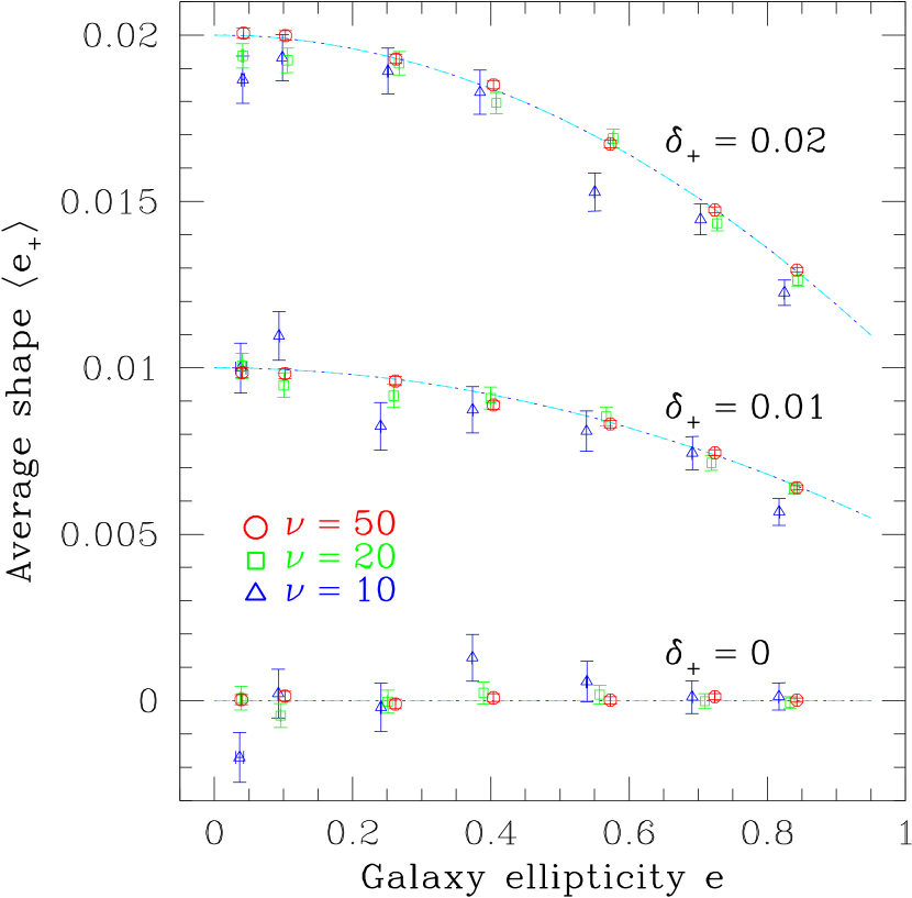
Figure 11: Average shape $\langle e_{+}\rangle$ obtained from a native fit ring test. The horizontal axis plots the measured galaxy ellipticity $e$. Each point is an average from $10^{5}$ galaxies, while the error bar represents the scatter in $\langle e_{+}\rangle$; the dot-dashed line indicates the expected signal ${\mathcal{R}}\delta_{+}$. The $\langle e_{\times}\rangle$ response, not shown in this plot, exhibit a similar response as for the case $\delta_{+}=0$, since $\delta_{\times}=0$.

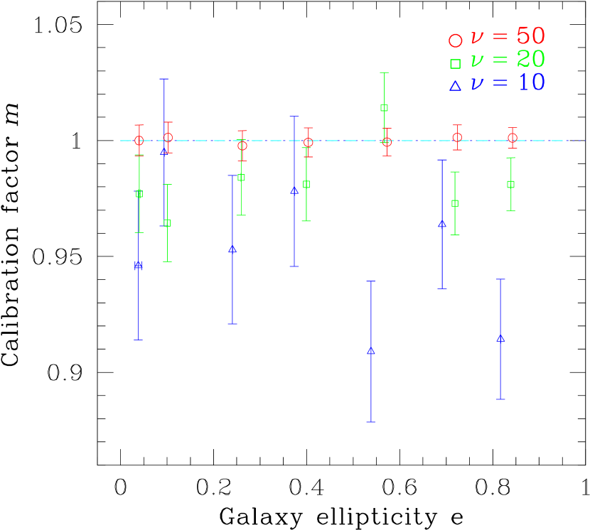
Figure 12: Calibration factor $m$ in native fits (no PSF). The vertical axis plots the normalized shear signal $\langle e_{+}\rangle/({\mathcal{R}}\delta_{+})$ from Figure 11 (the data for $\delta_{+}=0.01$ and $0.02$ have been combined). The offset from unity is the calibration error.

5.3 Accuracy for Asymmetric Galaxies

The previous section discussed shape measurement accuracies with a well defined input shape and high degree of symmetry. However, real galaxy images do not have an unambiguous shape nor a perfect exponential radial profile.

In this section, we measure the shapes of asymmetric galaxy images that have irregular isophotes (§4.2), for which there are no unambiguous definition of shape. However, in weak lensing, it is not the accuracy of the individual shape measurement, but rather the ability to recover the shear from an ensemble of shapes, that is well-defined and needs to be accurate. In this sense, the ring test provides a measure of accuracy for assigning a shape for these irregular galaxies.

In the ring test, the shape $e$ is determined by GLFit measurements; the same image, before pixelization, is rotated by a series of angles equally spaced between $0<\beta<2\pi$. Each rotated image is then sheared by $\delta_{+}=0$, $0.01$ or $0.02$, then pixelized for the ring test. With $100$ different orientations and $1,000$ (or more) realizations each, the uncertainty in the mean shape is $\sigma_{\delta_{+}}=\sigma_{e_{+}}/\sqrt{10^{5}}$, where $\sigma_{e_{+}}$ is the scatter in the $e_{+}$ measurements due to photon statistics. The ring test has no intrinsic-shape noise.

We test both the native and deconvolution fit cases at a series of different significance $\nu$, resolution $r_{b}$, and galaxy ellipticity $e$. The asymmetric galaxies of different shape $e$ are distinct combinations of exponential-disk and deVaucouleur profiles; they are not sheared versions of the same underlying shape.

Additionally, the shear calibration factor $m$ and additive bias $c$ can be measured with the ring test. The additive bias is the non-zero offset of the average shape when setting $\delta=0$ in the ring test, and is typically present when $e_{\rm PSF}\neq 0$. The calibration factor $m$ is then obtained by repeating the ring test with $\delta\neq 0$.

5.3.1 Native Fits

Figure 11 shows the mean shape $\langle e_{+}\rangle$ as a function of the galaxy ellipticity $e$ for native fits. The mean shape is expected to follow the curve ${\mathcal{R}}\delta_{+}$. The approximation ${\mathcal{R}}=1-{e^{2}}/{2}$, valid to ${\mathcal{O}}(\delta^{3})$, is more than adequate here. For the various significance ($\nu=10$, $20$, or $50$), the mean shape follows the expected curve very well. In particular, we see that there is no significant additive bias $c$ seen in the $\delta_{+}=0$ data points, to an uncertainty of $\sigma_{c}=\frac{0.01}{\nu}$.

Figure 12 plots the calibration factor $m$ by normalizing $\langle e_{+}\rangle$ for the $\delta_{+}\neq 0$ cases to the expected signal ${\mathcal{R}}\delta_{+}$, $m=\langle e_{+}\rangle/({\mathcal{R}}\delta_{+})$. The calibration is well within 1% of unity at $\nu=50$, but at lower detection significance, there is a systematic underestimation of the order $m\simeq 1-0.5/\nu$.

5.3.2 Deconvolution Fits

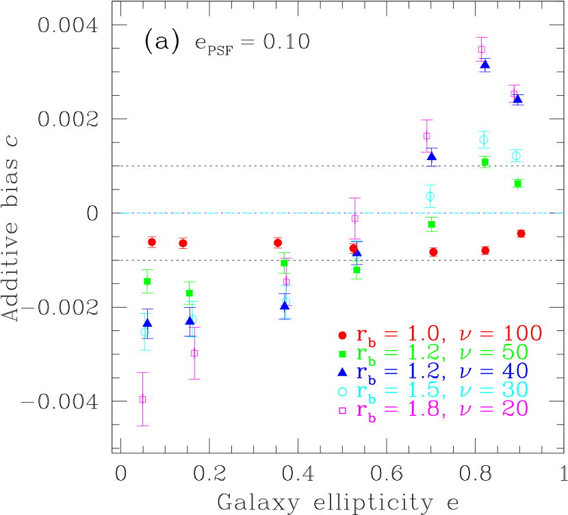
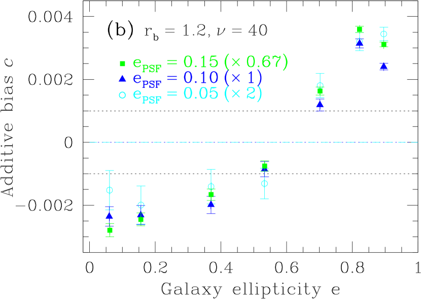
Figure 13: Additive bias $c$ due to PSF anisotropy. The average shape $\langle e_{+}\rangle$ is obtained from a deconvolution fit ring test with an Airy PSF of $e_{\rm PSF}=0.1$ for $\delta_{+}=0$, at various significance $\nu$ and resolution $r_{b}$. The average shape is expected to lie at zero (dot-dashed line); the offset from zero is the additive bias $c$. The dotted lines indicate $\pm 1\%$ of the PSF anisotropy. Each point is an average of $10^{5}$ galaxies. (a) Additive bias at $e_{\rm PSF}=0.10$, for various $(\nu,r_{b})$ pairs. (b) Additive bias at $(r_{b}=1.2,\ \nu=40)$ for $e_{\rm PSF}=0.05,0.10$ and $0.15$, with a scaling factor normalized to $e_{\rm PSF}=0.10$.

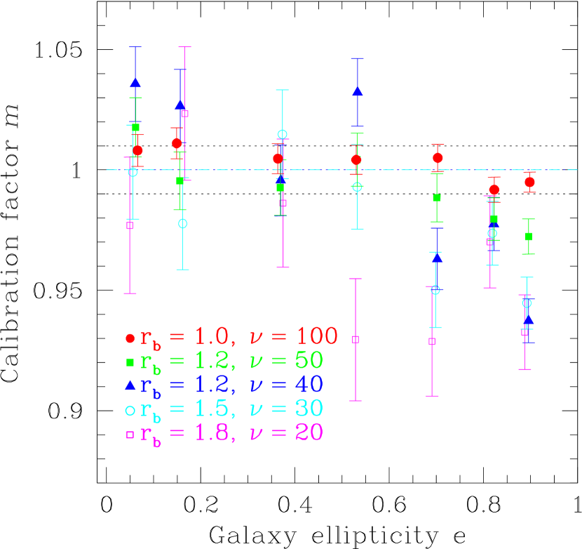
Figure 14: Multiplicative bias in deconvolution fits, for various $(\nu,r_{b})$ pairs. The shear is $\delta_{+}=0.02$, and the Airy PSF is circular, $e_{\rm PSF,+}=0$. Each point is an average of $10^{5}$ galaxies. The dotted line above and below indicate $\pm 1\%$ of the shear. (Currently running more simulations to decrease the error bar.)

The ring test with asymmetric galaxies is similarly performed with deconvolution fits, with a circular Airy PSF of $e_{\rm PSF}=0$ and an elliptical PSF with $e_{\rm PSF}=0.1$. Figure 13 shows the additive bias $c$ in the shape average $\langle e_{+}\rangle$ when $\delta_{+}=0$ and $e_{\rm PSF}=0.1$, while Figure 14 show the calibration factor $m$ for $\delta_{+}=0.02$. Both Figures show various cases of $(r_{b},\nu)$ pairs, which traces the $99\%$ convergence contour from Figure 4.

Figure 13 (a) shows $c$ as a function of $e$ at various $(r_{b},\nu)$ pairs. There is an $e$ dependence to the additive bias, which increases in magnitude with decreasing $\nu$. Comparing with Figure 9, we see that the additive bias is essentially identical to the PSF bias found in symmetric galaxies, indicating that the PSF bias is independent of the galaxy symmetry, or the orientation of the galaxy shape over the ensemble average. Figure 13 (b) shows that for a given $(r_{b},\nu)$, the additive bias $c$ scales linearly with $e_{\rm PSF}$ for reasonable $e_{\rm PSF}$ values.

Figure 14 shows the calibration factor $m$ for $e_{\rm PSF}=0$, $\delta_{+}=0.02$. At $\nu=100$ and better, the measured shear is within $1\%$ of the input shear signal. As the significance decreases ($\nu\leq 50$), there is a multiplicative bias for galaxy shapes over $e\,\raisebox{-3.44444pt}{$\stackrel{{\scriptstyle\textstyle>}}{{\sim}}$}\,0.6$, whose magnitude is about $-2.5\%$ at $e=0.8$ (axis ratio $a/b=3$). Similar results are found for $m$ for the case $e_{\rm PSF}\neq 0$, where $m=(\langle e_{+}\rangle-c)/{\mathcal{R}}\delta_{+}$, but with increased error bars due to the additional uncertainty in $c$.

6 Discussion

6.1 Limitations of GLFit and Implication to WL Surveys

There are limitations to GLFit with implications for WL surveys. If GLFit is to be used for shape analysis, the sampling rate must be such that the PSF minor-axis FWHM is sampled by $\geq 2.8$ pixels; otherwise, GLFit fails to converge to a unique shape (§5.1.1).

Similarly, the PSF-smeared objects which produce useful shapes must have a minimum resolution that depends on the significance (or vice-versa) in order to converge to a measurement of the pre-seeing galaxy shape. If we require shape measurements of all values of $e$ to be successful, then $r_{b}\geq 1.8$ is required at $\nu=20$, or $r_{b}\geq 1.2$ at $\nu\geq 40$ (§5.1.2). This implies that improvements in WL statistical accuracy are rapidly limited by the resolution of the galaxies: although going deep in the exposure increases the $S/N$ of the detected objects and reduces the scatter and systematic in the shear estimate, the required $S/N$ grows very rapidly for poorly resolved images, and it becomes difficult to produce additional useful WL data for poorly resolved galaxies.

We have also found that larger, well resolved galaxies ($r_{b}\raisebox{-3.44444pt}{$\stackrel{{\scriptstyle\textstyle>}}{{\sim}}$}\,5$) exhibit a problem with the deconvolution method when the PSF is an Airy function, due to the poor approximation of the Airy-functions wings by the GL expansion. A simple remedy is available: smooth the PSF and galaxy images before measuring both. Another solution is to choose an alternative to Gauss-Laguerre as the PSF decomposition basis functions, one that is better suited to describe an Airy function. However, a non-GL decomposition will make the deconvolution process excessively complex; another solution is to apodize the telescope to suppress the Airy wings.

6.2 Comparison to Other Methods

Kuijken (2006) offers an excellent description of the difference between various WL techniques; we refer the reader to this paper for the difference between, for example, the KSB method and Kuijken’s method, which is applicable to the difference bewteen KSB method and the EGL method.

Our EGL method is similar to Kuijken’s polar shapelet method (Kuijken, 2006). What the methods have in common are: the deconvolution of the PSF, which in principle allows for any PSF effects to be removed; forward fitting, which allows error propagation, and hence an error estimate to the measured shape; and the definition of shape as shear, which has a well-defined shear transformation. All of these features contribute to a better shear accuracy.

The differences between EGL and Kuijken’s methods are subtle. The first difference is that Kuijken method works the deconvolution and shearing in shapelet-coefficient space. Our EGL method determines the shape-as-shear by iteratively fitting within the pixel space. Secondly, Kuijken’s method obtains the shape using a shear transformation valid to first-order in $e$, which can be off by up to 10% at $e\simeq 0.9$ ($g=0.6$). Our method uses basis functions that are elliptical, i.e. the shear transformation is valid to all orders, which allows for the shape to be measured accurately for any $e$. The third difference is that, in Kuijken’s method, only the $m=0$ terms are used to describe the galaxy. This allows for less coefficients needed, and hence is efficient. In comparison, our method obtains the full set of coefficients to the specified order, which theoretically is more accurate under shearing or deconvolution. Another difference is in the choice of scale radius. Kuijken’s method uses 1.3 times the best-fit Gaussian $\sigma$ for the basis function scale radius, which apparently is optimal for the first-order method; EGL uses the best-fit elliptical Gaussian size, which gives the optimal sensitivity to small shear (BJ02 §3.1).

Unlike the KSB method, our EGL deconvolution method, the Kuijken (2006) polar shapelet and the Kaiser (2000) methods do not rely on the approximation that the PSF is circular up to a small linear “smear.” These methods are expected to do well on theoretical grounds; their differences (at least with Kuijken, 2006) seem to matter at the 1% level.

6.3 Comparison to Other Tests

As mentioned earlier, the main difference between this paper and previous end-to-end tests (Erben et al., 2001; Bacon et al., 2001; STEP, ) is that we test the individual steps of the analysis. The difference is mainly in the distribution of galaxies: these end-to-end tests mimic the distribution to an actual WL field image, while we test at specific S/N and galaxy size (resolution) sets. By controlling the exact distribution of galaxy shapes, we also eliminate shape noise in the shear estimate, and are able to quantify the effect that noise or resolution/sampling has on the shear.

The main differences from other “dissection” methods (HS, 03; Kuijken, 2006) are the inclusion of and quantifying noise effects, testing with asymmetric galaxies, and determining the limits of shape-measurement convergence. HS (03) demonstrates the calibration errors for a variety of PSFs (Gaussian, seeing-limited, diffraction-limited), while we only test for Airy PSFs as the worst-case scenario. In HS (03), the galaxy types were varied as well (Gaussian, Exponential, deVaucouleurs), but they are symmetric, which can mask potential problems in shape measurements. Their simulation focuses on the calibration accuracy, but does not quantify the additive error or include noise effects. Kuijken (2006) includes an analysis with noise, but does not quantify them; a variety of Sersic indices (for galaxies) are tested, but are symmetric. Their PSFs do not test the diffraction-limited (Airy) case, although asymmetric PSFs, which are not considered in this paper, are tested.

6.4 Accuracy with EGL Method

With the EGL method, the systematic due to the shape measurement method is well under the 0.1% level under ideal native-fit conditions, where the galaxy is symmetric and PSF is absent, as long as the minimum sampling and S/N criteria (minor axis width $>2.8$ pixels, $\nu>10$) are met.

The deviation from this high accuracy comes from real-life complications. In native fits, when the galaxies are not elliptically symmetric, the shear calibration factor degrades by $\sim-0.5/\nu$ as S/N is decreased.

The presence of a PSF further complicates the matter; deconvolution with PSFs of truncated coefficients becomes a source of error for well-resolved objects with an Airy PSF (up to 0.5%), but solutions to this poor approximation of the PSF are straightforward. More generally, the circularly-symmetric Airy PSF itself introduces an $e$ dependent systematic in the calibration factor, at worst $\sim-3\%$ at $e=0.8,\;\nu=20$. A non-circular PSF adds a shear additive error that is proportional to the shape of the PSF, which also increases with decreasing S/N (up to $\pm 3\%$ of $e_{\rm PSF}$ at $\nu=20$). For the deconvolution fits, the sign and magnitude of the calibration and additive error is approximately the same for both the symmetric and asymmetric galaxies.

The systematics are typically inversely proportional to the S/N. At high S/N ($\nu>50$), we have calibration error $\raisebox{-3.44444pt}{$\stackrel{{\scriptstyle\textstyle<}}{{\sim}}$}1\%$, and the PSF anisotropy is $>99\%$ suppressed. These errors become $\sim 4\%$ problems as $\nu\rightarrow 20$. The systematics are a function of the galaxy shape itself as well, with the systematic at low $e$ having the reverse sign of that at high $e$.

To attain 0.1% accuracy that is desired in future WL surveys, it is obvious that this shape measurement method itself needs to be refined. In addition, the whole pipeline needs to be rid of any systematics that are unrelated to the shape measurement, such as crowding or selection effects.

7 Conclusion

The elliptical Gauss-Laguerre decomposition is one of the most stringently tested methods to characterize shapes of galaxies. With the EGL decomposition, shapes are measured without the need for empirical shear/smear polarizabilities, and PSFs are removed by deconvolution. The shear, obtained from averaging an isotropic ensemble of galaxy shapes, is highly accurate due to the definition of shape as shear.

We have demonstrated that the EGL method allows shear recovery of unprecedented accuracy, and quantified its degradation due to PSF, truncation of the EGL decomposition, image noise, and sampling rate/resolution. However, the current work is limited to the extraction of shapes; further work, including the full pipeline analysis, is required for attaining 0.1% accuracy in shear estimation.

References

- Bacon et al. (2001) Bacon, D. J., Refregier, A., Clowe, D., & Ellis, R. S. 2001, MNRAS, 325, 1065
- Bartelmann & Schneider (2001) Bartelmann M., & Schneider P., 2001, Phys. Rep. 340, 291
- Berry et al. (2004) Berry, R. H., Hobson, M. P., & Withington, S. 2004, MNRAS, 354, 199
- BJ (02) Bernstein, G. M., & Jarvis, M. 2002, AJ, 123, 583 (BJ02)
- Bertin & Arnouts (1996) Bertin, E. & Arnouts, S, 1996, A&AS 117, 393
- Bridle et al. (2002) Bridle, S., Kneib, J.-P., Bardeau, S., & Gull, S. 2002, The shapes of galaxies and their dark halos, Proceedings of the Yale Cosmology Workshop “The Shapes of Galaxies and Their Dark Matter Halos”, New Haven, Connecticut, USA, 28-30 May 2001. Edited by Priyamvada Natarajan. Singapore: World Scientific, 2002, ISBN 9810248482, p.38, 38
- Erben et al. (2001) Erben, E., van Waerbeke, L., Bertin, E., Mellier, Y., & Schneider, P. 2003, A&A, 366, 717
- Fischer et al. (1997) Fischer, P., Bernstein, G., Rhee, G., & Tyson, J. A. 1997, AJ, 113, 521
- (9) Heymans, C., et al., 2005, astro-ph/0506112
- HS (03) Hirata, C. & Seljak, U. 2003, MNRAS, 343, 459
- van Waerbeke et al. (2005) van Waerbeke, L., Mellier, Y., & Hoekstra, H. 2005, A&A, 429, 75
- Jain et al. (2006) Jain, B., Jarvis, M., & Bernstein, G. 2006, Journal of Cosmology and Astro-Particle Physics, 2, 1
- Jarvis et al. (2003) Jarvis, M., Bernstein, G., Jain, B., Fischer, P., Smith, D., Tyson, J. A., and Wittman, D., 2003, AJ, 125, 1014
- Kaiser (2000) Kaiser, N., 2000, ApJ, 537, 555
- Kaiser, Squires, & Broadhurst (1995) Kaiser, N., Squires., G., & Broadhurst., T., 1995, ApJ, 449, 460 (KSB)
- Kuijken (2006) Kuijken, K. 2006, A&A (submitted) astro-ph/0601011
- Ma et al. (2006) Ma, Z., Hu, W., & Huterer, D. 2006, ApJ, 636, 21
- Massey et al. (2004) Massey, R., et al. 2004, AJ, 127, 3089
- Miralda-Escudé (1991) Miralda-Escudé, J. 1991, ApJ, 380, 1
- Refregier & Bacon (2003) Refregier, A. & Bacon, D.J. 2003, MNRAS, 338, 48