ULTRACAM observations of SDSS J170213.26+322954.1– an eclipsing cataclysmic variable in the period gap

Abstract

We present high-speed, three-colour photometry of the eclipsing cataclysmic variable SDSS J170213.26+322954.1 (hereafter SDSS J1702+3229). This system has an orbital period of 2.4 hours, placing it within the “period gap” for cataclysmic variables. We determine the system parameters via a parameterized model of the eclipse fitted to the observed light curve by $\chi^{2}$ minimization. We obtain a mass ratio of $q=0.215\pm 0.015$ and an orbital inclination $i=82^{\circ}.4\pm 0^{\circ}.4$. The primary mass is $M_{\mathrm{w}}=0.94\pm 0.01M_{\sun}$. The secondary mass and radius are found to be $M_{\mathrm{r}}=0.20\pm 0.01M_{\sun}$ and $R_{\mathrm{r}}=0.243\pm 0.013R_{\sun}$ respectively. We find a distance to the system of $440\pm 30$  pc, and an effective temperature for the secondary star of $3800\pm 100$K (corresponding to a spectral type of M0$\pm$0.5V). Both the distance and effective temperature are consistent with previous values derived via spectroscopy of the red star.

The secondary star is significantly less massive than expected for the orbital period, and significantly warmer than expected for its mass. This can be explained if the secondary star is significantly evolved: the mass and effective temperature are consistent with a secondary star that began mass transfer with a greatly reduced central hydrogen fraction. The nature of the secondary star in SDSS J1702+3229 supports predictions that CVs with evolved secondary stars might be found accreting within the period gap.

1 Introduction

Cataclysmic variable stars (CVs) are a class of interacting binary system undergoing mass transfer via a gas stream and accretion disc from a Roche-lobe filling secondary to a white dwarf primary. A bright spot is formed at the intersection of the disc and gas stream, giving rise to an ‘orbital hump’ in the light curve at phases $0.6-1.0$ due to foreshortening of the bright-spot. Warner (1995) gives a comprehensive review of CVs. The light curves of eclipsing CVs can be quite complex, with the accretion disc, white dwarf and bright-spot all being eclipsed in rapid succession. With sufficient time-resolution, however, this eclipse structure allows the system parameters to be determined to a high degree of accuracy (Wood et al., 1986).

SDSS J1702+3229 is a deeply eclipsing CV, first discovered through the Sloan digital sky survey (Szkody et al., 2004). The spectrum is highly suggestive of a dwarf-nova type system, a fact confirmed by its recent outburst during which it exhibited 0.3 mag superhumps (VSNET alert 8715), placing it amongst the SU UMa sub-class of Dwarf Novae. The system is particularly worthy of study, as its orbital period of 2.4 hours places it squarely within the period gap. Furthermore, its deeply eclipsing nature allows accurate system parameters to be derived. As such, SDSS J1702+3229 constitutes an excellent test of evolutionary models for CVs, which predict secondary star masses and radii for systems within the gap.

In this paper we present ultracam $u^{\prime}g^{\prime}r^{\prime}$ lightcurves of SDSS J1702+3229, and use these lightcurves to derive the system parameters. The observations are described in section 2, the results are presented in section 3, and discussed in section 4.

2 Observations

Table 1: Journal of observations. Observing conditions were clear except for 25^th Aug 2005, when thin cirrus was present. The dead-time between exposures was 0.025 s for all observations. The GPS timestamping on each data point is accurate to 50 $\mu$s.

Date	Start Phase	End Phase	Filters	Exposure time (s)	Data points	Eclipses	Seeing (arcsec)	Airmass
2005 Aug 11	-0.24	1.28	u′g′r′	1.62	7922	2	0.6–2.5	1.00–1.44
2005 Aug 12	9.80	10.31	u′g′r′	1.62	2709	1	0.6–0.8	1.00–1.05
2005 Aug 14	29.86	30.30	u′g′r′	1.62	2335	1	0.6–1.2	1.01–1.06
2005 Aug 15	39.72	40.29	u′g′r′	1.62	3040	1	0.7–1.2	1.00–1.07
2005 Aug 25	139.65	139.70	u′g′r′	1.62	372	0	0.6–1.2	1.02–1.03
2005 Aug 25	139.70	140.28	u′g′r′	2.46	2013	1	0.7–1.2	1.03–1.17

On nights between Aug 11^th 2005 and Aug 25^th 2005, SDSS J1702+3229 was observed simultaneously in the SDSS-$u^{\prime}g^{\prime}r^{\prime}$ colour bands using ultracam (Dhillon & Marsh, 2001) on the 4.2-m William Herschel Telescope (WHT) on La Palma. The observations were taken between airmasses of 1.0–1.4, in typical seeing conditions of 1.2 arcsecs, but with a range of 0.6–2.5 arcsecs. With the exception of the night of Aug 25^th 2005, when thin cirrus was present, the data were taken in photometric conditions, albeit with heavy dust extinction ($\sim$1 mag at zenith). Six eclipses were observed in total. Data reduction was carried out in a standard manner using the ultracam pipeline reduction software, as described in Feline et al. (2004), and a nearby comparison star was used to correct the data for transparency variations.

3 Results

3.1 Orbital Ephemeris

Table 2: Mid-eclipse timings (HJD + 2453594). The negative cycle timings are by-eye estimates from Szkody et al. (2004), The uncertainties for the values measured from our eclipses are 1.0$\times 10^{-5}$.

Cycle No.	u′	g′	r′
-7701	-770.341 $\pm$ 0.002
-7700	-770.240 $\pm$ 0.002
-7699	-770.140 $\pm$ 0.002
0	0.39201	0.39204	0.39206
1	0.49204	0.49208	0.49210
10	1.39289	1.39285	1.39284
30	3.39447	3.39449	3.39448
40	4.39529	4.39528	4.39530
140	14.40349	14.40354	14.40353

The times of white dwarf mid-ingress $T_{\mathrm{wi}}$ and mid-egress $T_{\mathrm{we}}$ were determined by locating the minimum and maximum times, respectively, of the light curve derivative. Mid-eclipse times, $T_{\mathrm{mid}}$, were determined by assuming the white dwarf eclipse to be symmetric around phase zero and taking $T_{\mathrm{mid}}=(T_{\mathrm{we}}+T_{\mathrm{wi}})/2$. These mid eclipse times were combined with a by-eye estimate of the mid-eclipse times from Szkody et al. (2004), and a linear least-squares fit to the mid-eclipse times was used to derive the ephemeris. The errors on the mid-eclipse times from Szkody et al. (2004) were estimated by-eye, and the errors on our mid-eclipse times were adjusted to give $\chi^{2}=1$, giving an ephemeris of:

$$\begin{array}[]{ccrcrl}\\ HJD&=&2453594.39209&+&0.10008209&E.\\ &&4&\pm&9&\end{array}$$

There was no evidence for a variation in $O-C$. This ephemeris was used to phase our data for the analysis which follows.

3.2 Lightcurve morphology and variations

Figure 1: The phase folded $u^{\prime}g^{\prime}r^{\prime}$ (from top to bottom) light curves of SDSS J1702. All six observed eclipses are shown superimposed to emphasise the variability between them.

Figure 1 shows the six observed eclipses of SDSS J1702, folded on the orbital phase. The white dwarf ingress and egress features are clearly visible, as are the ingress and egress features of the bright spot (see chapter 2.6.2 of Warner, 1995, for an illustrated example of an eclipse in a typical dwarf nova system). The eclipses are not total, and there is significant uneclipsed flux in the $g^{\prime}$ and $r^{\prime}$ bands, suggesting the secondary star contributes significantly at these wavelengths.There are significant drops in the amount of variability seen in the lightcurves at phases corresponding to the ingress of the bright spot, and the white dwarf. From this we can conclude that there is substantial flickering from both the inner disc and the bright spot. This finding is consistent with the results of Bruch (2000), who found that the bright spot and inner disc were the most common sites of flickering in cataclysmic variables. There is some suggestion for variation in the shape of the orbital hump around phase 0.8. Such variability suggests a change in large-scale structure within the bright spot on a timescale of days. The eclipses also show changes in the flux levels and slopes between phases 1.04–1.08, which is strong evidence for varying disc fluxes and brightness profiles. There is no evidence for variation in the size or duration of white dwarf egress, as might be expected if the white dwarf is surrounded by a boundary layer of varying thickness or flux.

3.3 A parameterized model of the eclipse

To determine the system parameters we used a physical model of the binary system to calculate eclipse light curves for each of the various components. Feline et al. (2004) showed that this method gives a more robust determination of the system parameters in the presence of flickering than the derivative method of Wood et al. (1986). We used the technique developed by Horne et al. (1994) and described in detail therein. This model assumes that the eclipse is caused by the secondary star, which completely fills its Roche lobe. A few changes were necessary in order to make the model of Horne et al. (1994) suitable for our data. The most important of these was the fitting of the secondary flux, prompted by the detection of a significant amount of flux from the secondary in the $g^{\prime}$ and $r^{\prime}$ bands. We fit the model to all the observed eclipses, which were phase-folded and binned into groups of 7 data points.

The 10 parameters that control the shape of the light curve are as follows:

1. The mass ratio, $q$.

2. The white dwarf eclipse phase full-width at half-depth, $\Delta\phi$.

3. The outer disc radius, $R_{\mathrm{d}}/a$.

4. The white dwarf limb-darkening coefficient, $U_{\mathrm{w}}$.

5. The white dwarf radius, $R_{\mathrm{w}}/a$.

6. The bright-spot scale, $S/a$. The bright-spot is modelled as a linear strip passing through the intersection of the gas stream and disc. The intensity distribution along this strip is given by $(X/S)^{2}e^{-X/S}$, where $X$ is the distance along the strip.

7. The bright-spot tilt angle, $\theta_{\mathrm{B}}$, measured relative to the line joining the white dwarf and the secondary star. This allows adjustment of the phase of the orbital hump.

8. The fraction of bright-spot light which is isotropic, $f_{iso}$.

9. The disc exponent, $b$, describing the power law of the radial intensity distribution of the disc.

10. A phase offset, $\phi_{0}$.

The amoeba algorithm (downhill simplex; Press et al. 1986) was used to adjust selected parameters to find the best fit. A linear regression was used to scale the four light curves (for the white dwarf, bright-spot, accretion disc and secondary) to fit the observed light curves in each passband. The data were not good enough to determine the white dwarf limb-darkening coefficient, $U_{\mathrm{w}}$, accurately. To find an appropriate limb-darkening coefficient, we obtained an estimate of the effective temperature and mass of the white dwarf from a first iteration of the method below, and assuming a limb-darkening coefficient of 0.5. The mass and effective temperature was then used in conjunction with the stellar atmosphere code of Gänsicke et al. (1995) to generate angle-dependent white dwarf model spectra. To convert the spectra to observed fluxes the model spectra were folded through passbands corresponding to the instrumental response in each filter; the effects of the SDSS filter set, the ultracam CCD responses and the dichroics used in the instrumental optics were taken into account. These fluxes were then fit as a function of the limb position in order to derive limb-darkening parameters for each band. The values adopted are given in table 3. A second iteration using these values for the limb-darkening parameter gave the final values for each parameter.

In order to estimate the errors on each parameter once the best fit had been found, we perturbed one parameter from its best fit value by an arbitrary amount (initially 5 per cent) and re-optimised the rest of them (holding the parameter of interest, and any others originally kept constant, fixed). We then used a bisection method to determine the perturbation necessary to increase $\chi^{2}$ by $1$, i.e. $\chi^{2}-\chi_{\mathrm{min}}^{2}=\Delta\chi^{2}=1$. The difference between the perturbed and best-fit values of the parameter gave the relevant $1\sigma$ error (Lampton, Margon & Bowyer, 1976).

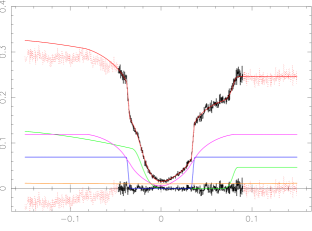
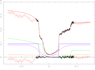
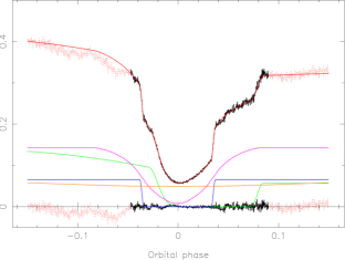
Figure 2: The phased folded $u^{\prime}g^{\prime}r^{\prime}$ (from top to bottom) light curves of SDSS J1702, fitted separately using the model described in section 3.3. The data (black) are shown with the fit (red) overlaid and the residuals plotted below (black). Below are the separate light curves of the white dwarf (blue), bright spot (green), accretion disc (purple) and the secondary star (orange). Data points neglected in the fit are shown in red (light grey).

Table 3: Parameters fitted using a modified version of the model of Horne et al. (1994). The fluxes of each component are also shown. Prior to fitting, the data were phase-folded and binned by seven data points. Note that the orbital inclination $i$ is not a fit parameter but is calculated using $q$ and $\Delta\phi$.

Band	u′	g′	r′
Inclination $i$	$82\aas@@fstack{\circ}0\pm 0\aas@@fstack{\circ}1$	$82\aas@@fstack{\circ}6\pm 0\aas@@fstack{\circ}1$	$82\aas@@fstack{\circ}6\pm 0\aas@@fstack{\circ}1$
Mass ratio $q$	$0.226\pm 0.002$	$0.210\pm 0.001$	$0.209\pm 0.001$
Eclipse phase width $\Delta\phi$	$0.0713\pm 0.0001$	$0.07126\pm 0.00003$	$0.0711\pm 0.0001$
Outer disc radius $R_{\mathrm{d}}/a$	$0.290\pm 0.003$	$0.288\pm 0.001$	$0.293\pm 0.001$
White dwarf limb darkening $U_{\mathrm{w}}$	$0.344\pm 0.008$	$0.267\pm 0.008$	$0.227\pm 0.003$
White dwarf radius $R_{\mathrm{w}}/a$	$0.0095\pm 0.0007$	$0.0096\pm 0.0001$	$0.0088\pm 0.0006$
bright-spot scale $S/a$	$0.043\pm 0.001$	$0.0338\pm 0.0004$	$0.040\pm 0.001$
bright-spot orientation $\theta_{\mathrm{B}}$	$161\aas@@fstack{\circ}4\pm 0\aas@@fstack{\circ}6$	$162\aas@@fstack{\circ}4\pm 0\aas@@fstack{\circ}3$	$161\aas@@fstack{\circ}4\pm 0\aas@@fstack{\circ}7$
Isotropic flux fraction $f_{iso}$	$0.36\pm 0.01$	$0.343\pm 0.003$	$0.410\pm 0.003$
Disc exponent $b$	$-1.1\pm 0.1$	$-1.1\pm 0.1$	$-1.0\pm 0.1$
Phase offset $\phi_{0}$	$57\pm 3\times 10^{-5}$	$60\pm 2\times 10^{-5}$	$57\pm 2\times 10^{-5}$
$\chi^{2}$ of fit	866	4634	3555
Number of datapoints $\nu$	1268	1268	1268
Flux (mJy)
White dwarf	$0.0690\pm 0.0010$	$0.0960\pm 0.0003$	$0.0654\pm 0.0004$
Accretion disc	$0.1191\pm 0.0010$	$0.0877\pm 0.0004$	$0.1427\pm 0.0005$
Secondary	$0.0126\pm 0.0004$	$0.0203\pm 0.0001$	$0.0629\pm 0.0002$
bright-spot	$0.1294\pm 0.0007$	$0.1418\pm 0.0002$	$0.1379\pm 0.0003$

The results of the model fitting are given in table 3 and shown in figure 2. It is apparent that the model is a very good fit to the data during eclipse. In particular, the ingress and egress features are well modelled. Further confidence in the results of the fitting is provided by the consistency in fitted parameters between wavebands (for example, the white dwarf radius and eclipse phase width). However, the model is a poor fit to the data prior to eclipse. Given the large changes seen in this part of the lightcurve between different eclipses (see figure 1), this is unsurprising, but it may also reflect the simple nature of the disc and bright spot in our model. To limit the effects that the poor fit to pre-eclipse data may have on the resulting system parameters we excluded the regions shown in red (light grey) in figure 2 from the fit. The exclusion of these regions from the fit can have a small effect on the derived value of the mass ratio, $q$. In our model, constraints on the mass ratio arise from the position of bright spot ingress and egress, but also from the height of the bright-spot hump seen before eclipse, and the shape of the lightcurve at mid eclipse. The net effect is that the values for $q$ derived from each band are marginally inconsistent, with a difference of around $4\sigma$. This inconsistency in $q$ produces a corresponding uncertainty in $i$, which depends upon $q$ and $\Delta\phi$. In the analysis that follows we assume that the scatter in $q$ between SDSS bands is indicative of the uncertainty in this parameter, and adopt values of $q=0.215\pm 0.01$ and $i=82\aas@@fstack{\circ}4\pm 0\aas@@fstack{\circ}4$, as shown in table 4.

We calculated the remaining system parameters following the method described in Feline et al. (2004). In brief, the white dwarf fluxes in table 3 are fitted using $\chi^{2}$ minimisation to white dwarf colours from the model atmospheres of Bergeron et al. (1995), converted to the SDSS system using the transformations of Smith et al. (2002); this provides an estimate of the white dwarf temperature. The white dwarf mass can then be derived using a white dwarf mass–radius relation, and the remaining system parameters are derived from the white dwarf mass and the results of the model fits. We used the Nauenberg mass-radius relation (Nauenberg, 1972). Because the Nauenberg relation applies to a cold, non-rotating white dwarf we applied a correction to the mass-radius relation, appropriate for the white dwarf temperature derived above. The radius of the white dwarf at $10000$ K is about 5 per cent larger than for a cold ($0$ K) white dwarf (Koester & Schoenberner, 1986). To correct from $10000$ K to the appropriate temperature, the white dwarf cooling curves of Wood (1995) for $M_{\mathrm{w}}/M_{\sun}=1.0$, the approximate mass given by the Nauenberg relation, were used. This gave a radial correction factor of $7.0$ per cent. A distance to the system was derived by comparing the white dwarf fluxes in table 3, and the predicted fluxes from Bergeron et al. (1995); the uncertainty in the distance is dominated by the uncertainty in the white dwarf temperature. The derived distance of $440\pm 30$ pc is consistent with the lower end of possible distances derived by Szkody et al. (2004) of 460–650 pc. The latter estimate was obtained by assuming the secondary star contributes 100% of the red light in the system, and so we might expect the true distance to lie towards the lower end of the range.

In addition, we attempted to derive an effective temperature for the secondary star, by fitting the secondary star fluxes to the colours of main-sequence stars. This method should be treated with caution, as the measured flux from the secondary star depends upon assumptions about the disc emission and bright-spot lightcurve. Indeed, comparison of the secondary star colours with the colours of main-sequence stars in the SDSS photometric system (Fukugita et al., 1996) showed that the $u^{\prime}-g^{\prime}$ colour was exceedingly blue for a main sequence star, given the $g^{\prime}-r^{\prime}$ colour. Working under the assumption that the $g^{\prime}-r^{\prime}$ colour is much less likely to be contaminated by disc and bright spot emission, we used $\chi^{2}$ minimisation to fit the $g^{\prime}-r^{\prime}$ colour to the colours of main-sequence stars as catalogued by Kenyon & Hartmann (1995). The effective temperature we derive agrees well with the spectral type of M1.5$\pm$1 derived from optical spectroscopy (Szkody et al., 2004), giving us confidence that the temperature is correct. The final adopted system parameters are shown in table 4.

Table 4: System parameters of SDSS J1702+3229 derived using the Nauenberg mass–radius relation corrected to the appropriate $T_{\mathrm{w}}$. $R_{\mathrm{r}}$ is the volume radius of the secondary’s Roche lobe (Eggleton, 1983). Except for the mass ratio and the inclination, which are discussed in section 3.3, the weighted means of the appropriate values from Table 3 are used for the system parameters.

Inclination $i$	$82\aas@@fstack{\circ}4\pm 0\aas@@fstack{\circ}4$
Mass ratio $q=M_{\mathrm{r}}/M_{\mathrm{w}}$	$0.215\pm 0.015$
White dwarf mass $M_{\mathrm{w}}/M_{\sun}$	$0.94\pm 0.01$
Secondary mass $M_{\mathrm{r}}/M_{\sun}$	$0.20\pm 0.01$
White dwarf radius $R_{\mathrm{w}}/R_{\sun}$	$0.0091\pm 0.0001$
Secondary radius $R_{\mathrm{r}}/R_{\sun}$	$0.243\pm 0.013$
Separation $a/R_{\sun}$	$0.948\pm 0.005$
White dwarf radial velocity $K_{\mathrm{w}}/\mathrm{km\;s^{-1}}$	$84\pm 6$
Secondary radial velocity $K_{\mathrm{r}}/\mathrm{km\;s^{-1}}$	$391\pm 1.0$
Outer disc radius $R_{\mathrm{d}}/a$	$0.290\pm 0.001$
White dwarf temperature $T_{\mathrm{w}}/\rm{K}$	$17000\pm 500$
Secondary star temperature $T_{\mathrm{r}}/\rm{K}$	$3800\pm 100$
Distance $d/\mathrm{pc}$	$440\pm 30$

4 Discussion

4.1 Superhump period excess and mass ratio

On the 3^rd Oct 2005, SDSS J1702+3229 entered its first recorded outburst (VSNET Alert 8709); On Oct 7^th, 0.3 mag superhumps were observed, with a superhump period $P_{sh}$ of 0.1056 days (VSNET Alert 8715). The detection of superhumps in this object is significant in the context of the well-established relationship between mass ratio and superhump period excess, as very few systems are available to calibrate the relationship at high mass ratios (Patterson et al., 2005).

From the reported superhump period and the orbital period reported in this paper we calculate a superhump period excess, $\epsilon=0.0551\pm 0.0005$. This is entirely consistent with the $\epsilon$–$q$ relationship established by Patterson et al. (2005) which predicts $\epsilon=0.052\pm 0.005$ for the mass ratio of SDSS J1702+3229.

4.2 Evolutionary status of the secondary star

Several independent theoretical studies predict the existence of a population of CVs with substantially evolved secondary stars (e.g Baraffe & Kolb, 2000; Andronov & Pinsonneault, 2004; Schenker et al., 2002; Podsiadlowski et al., 2003). Under the disrupted magnetic braking model of CV evolution, the period gap is caused by a cessation of magnetic braking which occurs when the secondary star becomes fully convective. The small central hydrogen abundance and higher central temperature of evolved stars imply lower radiative opacities; this naturally favours radiative transport. Sufficiently evolved secondary stars do not, therefore, become fully convective until they have evolved to shorter periods than the upper edge of the period gap. For sufficiently evolved secondary stars, the system can continue accreting throughout the gap (Baraffe & Kolb, 2000). We might therefore expect that a sizeable proportion of CVs with periods inside the period gap would possess evolved secondary stars.

Evidence that the secondary star in SDSS J1702+3229 has undergone significant nuclear evolution comes from two independent lines of argument; the secondary star is both too warm and insufficiently massive to be an ordinary star, given its orbital period. In this paper, we find an effective temperature for the secondary star of $3800\pm 100$ K, which agrees well with the reported spectral type of M1.5$\pm$1, or $3600\pm 200$ K (Szkody et al., 2004), derived from the TiO band spectral index derived by Reid et al. (1995). An effective temperature of 3800 K is too warm for a non-evolved CV secondary star at an orbital period of 2.4 hours (Baraffe & Kolb, 2000). At periods of around 3 hours, a typical spectral type is approximately M4 (c. f.  U Gem and IP Peg), whereas a spectral type of M1 is more typical of periods near 5 hours (see Smith & Dhillon, 1998, for examples). On the other hand, the early spectral type is consistent with a secondary star which has undergone significant nuclear evolution. From figure 3 of Baraffe & Kolb (2000), it is clear that the effective temperature of the secondary star in SDSS J1702+3229 is consistent with models of a secondary star that began mass transfer with a greatly reduced central hydrogen fraction.

The mass of the secondary star at a given orbital period is also indicative of the evolutionary state; the secondary mass is, to first order, a simple function of the period and the mass-radius relationship (see Howell et al., 2001, for example). The consequence of this is that an evolved secondary star will be under-massive for a given period, compared with the expected mass of a main-sequence secondary star. In fact, this is precisely what we observe; adopting the main-sequence mass-radius relationship of Chabrier & Baraffe (1997), we find the secondary star mass at a period of 2.4 hours should be $0.25M_{\sun}$. In this paper we find a secondary star mass of $M_{\mathrm{r}}=0.20\pm 0.01M_{\sun}$, which is significantly lower than expected for a main sequence star.

It is worth spending some time speculating upon the origin and subsequent evolution of SDSS J1702+3229. Clearly the secondary star has undergone significant nuclear evolution; the requirement for this to happen within a Hubble time implies that the initial mass of the secondary should be greater than 0.8$M_{\sun}$. What happened to the system after contact depends upon the secondary mass and upon the evolutionary state of the secondary at contact; for a primary mass of 0.94$M_{\sun}$, an initial secondary mass of 1.2$M_{\sun}$ or less implies that mass transfer from a main sequence star will be both thermally and dynamically stable (Politano, 1996). However, if the secondary star had already left the main sequence before contact, or was more massive than 1.2$M_{\sun}$, then the system would have undergone a phase of thermal timescale mass transfer. During this phase the orbit would shrink rapidly. Once mass transfer regained stability, the system would become recognisable as a CV at a much lower period. This channel raises the possibility that SDSS J1702+3229 might have emerged from thermal timescale mass transfer within the period gap. The accurate values of secondary mass, radius and effective temperature presented here should allow detailed modelling to recover the evolutionary past of SDSS J1702+3229, however this is beyond the scope of this paper. The future evolution of SDSS J1702+3229 depends sensitively on the evolutionary state of the secondary star. However, comparison with the models of Podsiadlowski et al. (2003) suggests that the system will evolve below the observed “period-minimum”, and may even be a progenitor of an AM CVn system.

4.3 Evolved secondary stars in CVs

A small number of CV systems now show very strong evidence for the presence of an evolved secondary star; both QZ Ser and EI Psc have unusually hot secondaries for their orbital period (Thorstensen et al., 002a, 002b), and the secondary star in EI Psc has a very large N/C abundance (Gänsicke et al., 2003). Indeed, the period of EI Psc is substantially below the period minimum, which is in principle only possible for an evolved secondary star. Given the difficulty in obtaining information about the secondary stars in CVs, it is at least plausible that systems with evolved secondary stars constitute a significant fraction of the CV population, although it is not yet possible to state whether the fraction is as high as 10%, as suggested by Podsiadlowski et al. (2003).

The existence of evolved secondaries amongst the cataclysmic variable population, and the fact that such systems may not show a period gap provides a natural explanation for the non-magnetic CVs found within the gap. It is tempting to speculate that most non-magnetic CVs within the period gap are explained by systems with evolved secondary stars. Given that the first such system which allows accurate determination of system parameters has an evolved secondary there may be some support for this hypothesis. Furthermore, such a hypothesis might explain the large fraction of systems within the period gap which exhibit superhumps (Katysheva & Pavlenko, 2003); superhumping systems must have mass ratios below a critical value of approximately 0.3, and the undermassive secondary stars in evolved systems would increase the proportion of systems with mass ratios which are unstable to superhumps.

We conclude that the secondary star in SDSS J1702+3229 shows evidence for significant nuclear evolution. The existence of a CV with an evolved secondary within the period gap supports predictions (e.g. Baraffe & Kolb, 2000) that CVs with evolved secondaries can continue accreting inside the period gap, and in some cases might show no period gap at all.

References

- Andronov & Pinsonneault (2004) Andronov N., Pinsonneault M. H., 2004, ApJ, 614, 326
- Baraffe & Kolb (2000) Baraffe I., Kolb U., 2000, MNRAS, 318, 354
- Bergeron et al. (1995) Bergeron P., Wesemael F., Beauchamp A., 1995, PASP, 107, 1047
- Bruch (2000) Bruch A., 2000, A&A, 359, 998
- Chabrier & Baraffe (1997) Chabrier G., Baraffe I., 1997, A&A, 327, 1039
- Dhillon & Marsh (2001) Dhillon V., Marsh T., 2001, New Astronomy Review, 45, 91
- Eggleton (1983) Eggleton P. P., 1983, ApJ, 268, 368
- Feline et al. (2004) Feline W. J., Dhillon V. S., Marsh T. R., Brinkworth C. S., 2004, MNRAS, 355, 1
- Feline et al. (2004) Feline W. J., Dhillon V. S., Marsh T. R., Stevenson M. J., Watson C. A., Brinkworth C. S., 2004, MNRAS, 347, 1173
- Fukugita et al. (1996) Fukugita M., Ichikawa T., Gunn J. E., Doi M., Shimasaku K., Schneider D. P., 1996, AJ, 111, 1748
- Gänsicke et al. (1995) Gänsicke B. T., Beuermann K., de Martino D., 1995, A&A, 303, 127
- Gänsicke et al. (2003) Gänsicke B. T., Szkody P., de Martino D., Beuermann K., Long K. S., Sion E. M., Knigge C., Marsh T., Hubeny I., 2003, ApJ, 594, 443
- Horne et al. (1994) Horne K., Marsh T. R., Cheng F. H., Hubeny I., Lanz T., 1994, ApJ, 426, 294
- Howell et al. (2001) Howell S. B., Nelson L. A., Rappaport S., 2001, ApJ, 550, 897
- Katysheva & Pavlenko (2003) Katysheva N. A., Pavlenko E. P., 2003, in ASP Conf. Ser. 292: Interplay of Periodic, Cyclic and Stochastic Variability in Selected Areas of the H-R Diagram SU UMa stars in the Period Gap. pp 255–+
- Kenyon & Hartmann (1995) Kenyon S. J., Hartmann L., 1995, ApJS, 101, 117
- Koester & Schoenberner (1986) Koester D., Schoenberner D., 1986, A&A, 154, 125
- Lampton et al. (1976) Lampton M., Margon B., Bowyer S., 1976, ApJ, 208, 177
- Nauenberg (1972) Nauenberg M., 1972, ApJ, 175, 417
- Patterson et al. (2005) Patterson J., Kemp J., Harvey D. A., Fried R. E., Rea R., et. al. 2005, PASP, 117, 1204
- Podsiadlowski et al. (2003) Podsiadlowski P., Han Z., Rappaport S., 2003, MNRAS, 340, 1214
- Politano (1996) Politano M., 1996, ApJ, p. 338
- Press et al. (1986) Press W. H., Flannery B. P., Teukolsky S. A., 1986, Numerical recipes. The art of scientific computing. Cambridge: University Press, 1986
- Reid et al. (1995) Reid I. N., Hawley S. L., Gizis J. E., 1995, AJ, 110, 1838
- Schenker et al. (2002) Schenker K., King A. R., Kolb U., Wynn G. A., Zhang Z., 2002, MNRAS, 337, 1105
- Smith & Dhillon (1998) Smith D. A., Dhillon V. S., 1998, MNRAS, 301, 767
- Smith et al. (2002) Smith J. A., Tucker D. L., Kent S., Richmond M. W., Fukugita M., Ichikawa T., Ichikawa S.-i., Jorgensen A. M., Uomoto A., Gunn J. E., Hamabe M., et al. 2002, AJ, 123, 2121
- Szkody et al. (2004) Szkody P., Henden A., Fraser O., Silvestri N., Bochanski J., et. al. 2004, AJ, 128, 1882
- Thorstensen et al. (002a) Thorstensen J. R., Fenton W. H., Patterson J., Kemp J., Halpern J., Baraffe I., 2002a, PASP, 114, 1117
- Thorstensen et al. (002b) Thorstensen J. R., Fenton W. H., Patterson J. O., Kemp J., Krajci T., Baraffe I., 2002b, ApJ, 567
- Warner (1995) Warner B., 1995, Cataclysmic Variable Stars. Cambridge University Press, Cambridge
- Wood et al. (1986) Wood J. H., Horne K., Berriman G., Wade R., O’Donoghue D., Warner B., 1986, MNRAS, 219, 629
- Wood (1995) Wood M. A., 1995, LNP Vol. 443: White Dwarfs, 443, 41