Tracing the Dynamical History of the Globular Cluster 47 Tucanae

Abstract

We use two stellar populations in the globular cluster 47 Tucanae to trace its dynamical history: blue stragglers and low mass main sequence stars. We assumed that the blue stragglers were formed through stellar collisions in all regions of the cluster. We find that in the core of the cluster, models of collisional blue stragglers agree well with the observations as long as blue stragglers are still continuing to form and the mass function in the cluster is extremely biased towards massive stars ($x=-8$ where a Salpeter mass function has $x=+1.35$). We show that such an extreme mass function is supported by direct measurements of the luminosity function of main sequence stars in the centre of the cluster. In the middle region of our dataset ($25^{\prime\prime}$ to $130^{\prime\prime}$ from the cluster centre), blue straggler formation seems to have stopped about half a Gyr ago. In the outskirts of the cluster, our models are least successful at reproducing the blue straggler data. Taken at face value, they indicate that blue straggler formation has been insignificant over the past billion years, and that a Salpeter mass function applies. However, it is more likely that the dominant formation mechanism in this part of the cluster is not the collisional one, and that our models are not appropriate for this region of the cluster. We conclude that blue stragglers can be used as tracers of dynamics in globular clusters, despite our incomplete understanding of how and where they were formed.

1. Introduction

Globular clusters in our Galaxy are often called the ideal laboratories for a variety of fields in stellar astrophysics. They provide the closest thing to controlled experiments in which to test theories of stellar evolution and stellar dynamics. From the evolution point of view, globular clusters provide a large population of stars that have a common distance, metallicity, and age. Under the assumption of single-star, undisturbed evolution, researchers have used globular clusters to test models of star formation and evolution of low-mass stars for decades. From the dynamics point of view, globular clusters lie in a very interesting region of phase space for stellar systems. Unlike open clusters, their crossing timescale is longer than their relaxation timescale, meaning that they do not dissolve quickly. Unlike galaxies, globular clusters have relaxation times shorter than their evolution time, meaning that they are dynamically evolved. Under the assumption of collisionless dynamical evolution, globular clusters are very nice real-life examples of large $N$ Newtonian gravitation systems.

If one looks at globular clusters very closely, their use as laboratories for stellar evolution and stellar dynamics becomes less obvious. The assumptions mentioned in the previous paragraph break down. Not all stars in globular clusters have evolved in isolation; not all stellar interactions in globular clusters are collisionless. Our laboratory is now a place to study the interplay between stellar dynamics and stellar evolution, and to look carefully at the feedback between these two fundamental fields of stellar astronomy.

In this paper, we attempt to use the effects of strong stellar encounters, particularly stellar collisions, to probe the dynamical history of the globular cluster 47 Tucanae. We will use two tracer populations to do this. The first is blue stragglers, core-hydrogen-burning stars that are bluer and brighter than the main sequence turnoff. The second population is the low-mass main sequence stars, specifically their mass function.

The effects of stellar collisions inside of dense globular clusters play a significant role in the evolution of these systems (Leonard, 1989). These collisions are one of a number of suspected mechanisms for producing blue stragglers. Many other mechanisms for the formation of these stars have been proposed, but the most convincing ideas involve close, disruptive encounters: direct collisions, or interactions within binary systems.

In a close binary, as the more massive star begins to swell on its path to becoming a red giant, some of its material may be pulled into the less massive star. This less massive star would then grow and become a blue straggler (McCrea, 1964). Close binary systems can also gradually lose angular momentum, forcing the two stars to combine into a blue straggler (Zinn & Searle, 1976). Most blue stragglers are more massive than the turnoff mass, but less than twice it, and these mechanisms are both able to account for these stars. However, both of these methods are unable to explain the presence of blue stragglers with masses greater than twice the turnoff mass, and this poses a significant problem for these explanations (Leonard & Linnell, 1992). Collisionally formed blue stragglers do not suffer from this problem, as it is possible, although rare, for three stars to collide, usually in an interaction involving a binary star system (Leonard, 1989). Direct measurements of masses of individual blue stragglers in globular clusters are rare, but the work of De Marco et al. (2005) suggests that $\sim 10$% of blue stragglers in globular clusters could be the result of triple collisions. Three of their 24 blue stragglers, with masses measured from HST STIS spectroscopy, have masses above 1.8 M_⊙. Interestingly, all 3 are within a few arcseconds of their cluster centres.

The main problem with the collisional mechanism is that it has been unable to explain all of the blue stragglers in any cluster. In particular, the collisional probability for a given star drops to near zero quite quickly outside of the core. For this reason, it has been suggested that blue stragglers are formed through both binary and collisional mechanisms (Mapelli et al., 2004; Davies et al., 2004). This suggestion is further supported by the findings of Piotto et al. (2004), who have shown that there is no correlation between expected collision rate and blue straggler frequency, and only minor correlations between this frequency and cluster mass and central density. As a cluster becomes more dense, stellar collisions become more likely, and blue stragglers formed through this method increase in number. The increased density, however, makes binary systems evolve faster due to exchanges of more massive stars in the binaries during dynamical interactions. If the rise in one mechanism’s efficiency is similar in magnitude to the drop in another’s, then this explains the lack of correlation between expected collision rate and blue straggler frequency (Davies et al., 2004).

In this paper, we examine the distribution of collisionally formed blue stragglers in the colour-magnitude diagram. Using Hubble Space Telescope (HST) and ground based observations of the globular cluster 47 Tuc, we are able to study blue stragglers in various regions of the cluster. We run simulations of the evolution of collisional blue stragglers, varying the mass function of their progenitor stars, as well as their formation times. We simulate three regions of the cluster, separated from each other by radial distance from the cluster centre, and find different formation times and progenitor mass functions for each. We discuss our data sets in section 2. In section 3, we give the details of our simulations. We show our results for each region of the cluster in section 4. Section 5 discuses mass segregation, and we summarize and discuss our results in section 6.

2. The Data

We use three sources of data to get as much coverage of 47 Tuc’s stellar populations as possible. Two of these sets are taken from HST images that cover the central region of the cluster. The third is ground-based data that covers the rest of the cluster, out to $1200^{\prime\prime}$ from the centre.

There are two HST imaging data sets analyzed in this paper: (1) archival Wide Field Planetary Camera 2 (WFPC2) data from program GO-6095 (PI: S. G. Djorgovski), consisting of F218W ($4\times 800$ s), F439W ($2\times 50$ s), and F555W (7 s) images; hereafter the “archival” data set; (2) ultra-deep WFPC2 data from Gilliland et al. (2000), consisting of $10^{5}$ s integration in each of the F555W and F814W bands. Sub-pixel dithering yields a point spread function whose full width at half maximum is approximately $0.07^{\prime\prime}$ on the PC1 CCD. Hereafter this will be referred to as the “ultra-deep” data set. An analysis of the archival and ultra-deep data sets is presented in the companion paper by Guhathakurta et al. (2006).

The blue stragglers from the archival dataset were selected from the data published in Piotto et al. (2002) and Piotto et al. (2004). We used the $B$ and $V$ magnitudes of each blue straggler (calculated from F439W and F555W magnitudes). We needed to know the absolute position of each blue straggler in RA and DEC, in order to combine this data set with the ground-based data. We used the STSDAS task ‘metric’ to convert from HST WPCS2 CCD coordinates. These data reach out to $130^{\prime\prime}$ from the cluster centre.

Our wide field data are taken from Ferraro et al. (2004), and cover the cluster out to $1200^{\prime\prime}$ from the centre. These data were taken using the Wide Field Imager on the 2.2 m ESO-MPI telescope at La Silla, and we have $B$, $V$, and $I$ magnitude information for each blue straggler. The HST image is more suited to analyzing the dense central region than the ground-based data. For this reason, the wide field data inside of $130^{\prime\prime}$ is not given in Ferraro et al. (2004), and is not used in our analysis.

The colour-magnitude diagram for 47 Tuc, taken from the archival WFPC2 data, is shown in Figure 1. The blue straggler selection box is shown as a solid line. This box encompasses the selection criteria used on both the HST and ground-based data.

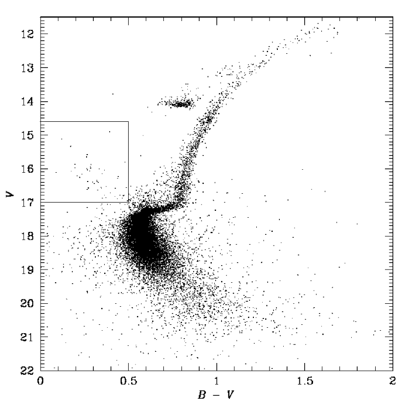
Figure 1.— The colour-magnitude diagram for 47 Tuc from the archival HST/WFPC2 data. The blue straggler selection box is marked.

We use the data from the archival and wide-field sources to plot both magnitude and colour against radial distance from the centre of the cluster, shown in Figures 2 and 3 respectively. The centre of the cluster is taken to be at Right Ascension $\rm 00^{h}24^{m}05.20^{s}$ and Declination $-72^{\circ}$04^′51.00^′′. The plot of magnitude against radial distance is in the B filter, colour against radial distance is in B-V, and the radial distance for both is given in the log of the distance in arc seconds. In both figures, there is an empty region from approximately $100^{\prime\prime}$ to $130^{\prime\prime}$. The shape of the HST field of view allows it to only cover a fraction of this area (Ferraro et al., 2004), and so no blue stragglers have been observed in this region.

Figure 2.— Apparent $B$ magnitude versus radial distance from the centre of the cluster, in the logarithm of arcseconds, for blue stragglers stars in our 47 Tuc sample. The number of bright blue stragglers dramatically declines outside the cluster core.

Figure 3.— The $B-V$ colour of 47 Tuc blue stragglers versus radial distance from the centre of the cluster, in the logarithm of arc seconds. Notice the lack of bluer blue stragglers at large distances from the cluster core.

In the magnitude plot, there is clearly a drop in the number of bright blue stragglers in the outskirts of the cluster. To determine the most statistically significant value of the radius at which this drop occurs, we used a Kolmogorov-Smirnov test to determine if the populations inside and outside of a given value of $r$ were drawn from the same parent population. We varied r from 1 to 150 arc seconds, in steps of 1 arc second. We found that the most statistically significant division is at $25^{\prime\prime}$, within the error of the $24^{\prime\prime}\pm 1.9^{\prime\prime}$ core radius of 47 Tuc (Howell, Guhathakurta, & Gilliland, 2000). The KS test returned a probability of more than 99.995% that the populations to the left and the right of the $25^{\prime\prime}$ line were drawn from different distributions. Bright blue stragglers are virtually non-existent outside of this region. A similar pattern is also apparent in the plot of colour against radial distance, indicating that the blue stragglers in the outer region of the cluster are cooler than those of the inner region.

We separate the data sets into three groups by radial distance from the centre of 47 Tuc. The colour-magnitude diagram of all the blue stragglers is shown in figure 4. The core of the cluster, consisting of stars from $0^{\prime\prime}$ to $25^{\prime\prime}$, contains the brightest and hottest stars and is shown as asterisks. The stars between $25^{\prime\prime}$ and $130^{\prime\prime}$, shown as circles, encompass the rest of the HST/WFPC2 coverage. The ground-based field of view, from $130^{\prime\prime}$ to $1200^{\prime\prime}$, contains none of the brighter or hotter stars, and is plotted as triangles. The core, middle region of our dataset, and ground-based field contain 44, 34, and 67 stars respectively. The open circles are blue stragglers from the middle region of our data that are bluer than any of our models, and the open triangles are blue stragglers that posed problems for our models in the outermost region of our data. Both populations will be discussed in detail in section 6.

Figure 4.— Colour-Magnitude diagram for all of the blue stragglers in our 47 Tuc sample. The core blue stragglers, between $0^{\prime\prime}$ and $25^{\prime\prime}$, are shown as asterisks; the blue stragglers that lie between $25^{\prime\prime}$ and $130^{\prime\prime}$ are shown as circles; and the outermost blue stragglers, between $130^{\prime\prime}$ and $1200^{\prime\prime}$ are shown as triangles. The open symbols highlight blue stragglers that pose problems for our simple collisional models, and will be discussed in detail in section 6.

3. Simulations

By assuming that all blue stragglers are created from single-binary collisions, where two of the stars involved merge, and using the method described in Sills & Bailyn (1999), we generate theoretical colour-magnitude diagrams of the blue straggler distribution in 47 Tuc. The probability of the colliding single star having a certain mass is taken from a power law mass function, representing the current mass function in the region of interest. This same mass function is used to find the probability of a binary system having a particular total mass. The mass of the secondary component of the binary is governed by a separate mass function, taken to have the Salpeter value of +1.35 as its index, which represents the mass function of the cluster when the binary was formed. All of these mass functions are of the form $dN/dM=M^{-(1+x)}$, where a Salpeter mass function has a value $x=+1.35$. The STARLAB software package is used to find the cross sections for binary-single collisions (McMillan & Hut, 1996).

Using the initial mass of the collision product, we interpolate an evolutionary track from the nearest simulated tracks. These simulated tracks are calculated using the Yale Rotational Stellar Evolution Code, YREC (Guenther et al., 1992). The initial conditions for the simulated tracks are generated with a smooth particle hydrodynamics simulations of colliding stars (Sills & Bailyn, 1999).

To produce a more accurate representation of the cluster, we are able to specify the time frame over which these stellar collisions occur. We alter the start and end times for a constant collision rate, and assume that the collision rate remains constant during this period as in Sills et al. (2000). This is still not an accurate representation of the dynamics of a cluster, but it allows us to generate reasonable models, and extract information on the approximate ages of the blue straggler populations. Finally, we weight each collision product evolutionary track by its probability of occuring, and generate a predicted blue straggler distribution in the colour-magnitude diagram.

The simulations require various values to be assumed. The velocity dispersion is taken 11 km s^-1 , and the binary fraction is set at 10%, within error of the predicted values (Gebhardt et al., 1995; Albrow et al., 2001). Both of these values have very little impact on the shape of the density function, and have a much larger effect on the total number of blue stragglers predicted. The metallicity of the cluster is more influential on the shape of the plot, and is set at $\rm[Fe/H]=-0.66$ (Gratton et al., 2003). Sills & Bailyn (1999) explore the effects of changing these quantities in detail.

Due to mass segregation, each of the three cluster regions, $0^{\prime\prime}$ to $25^{\prime\prime}$, $25^{\prime\prime}$ to $130^{\prime\prime}$, and $130^{\prime\prime}$ to $1200^{\prime\prime}$, could have very different mass functions. To improve the accuracy of our models, we simulate each region using a variety of mass function indices. We make the unphysical but simple assumption that the mass function remains constant in time over the entire simulation, and that, within each region, it does not change with distance from the core. This assumption is reasonable for clusters, like 47 Tuc, with short relaxation times. Most mass segregation will occur early in the cluster’s lifetime, before our simulations begin. By varying both the collision time frame, and mass function of the constituent stars, we find the best model for each region.

4. Results

4.1. The Core of 47 Tucanae

As can be seen in Figure 5, the innermost region of 47 Tuc contains the brightest blue stragglers in the cluster. The concentration of these stars is weighted much more toward the brighter and bluer end of the diagram than either of the other two areas, suggesting that the core population contains the most massive, and youngest, blue stragglers.

To find an accurate model of the $0^{\prime\prime}$ to $25^{\prime\prime}$ region, we generate colour-magnitude diagrams for a variety of collision time-frames. We find that the models that best approximate this area are those that start collisions at some time in the past and continue to the current time. The brightest blue stragglers rapidly evolve out of the blue straggler region of the colour-magnitude diagram, and stopping the collisions a short time ago leaves this area void of any stars.

We test various start times for the collision process, and find that the core of 47 Tuc has probably been producing blue stragglers for at least the past 7 Gyr. Comparing the observed distribution of blue stragglers with our models using a two-dimensional Kolmogorov-Smirnov test, we find that at a start time of 7 Gyr ago, the best fitting model is produced. More recent start times rapidly drop in their ability to reproduce observations. Starting the collision process further back than this produces models that are almost as closely fitting to the data.

Upon establishing the time frame over which the collisions occur, we test various mass functions and find the best-fitting slope. With a mass function of $-8$ and with collisions occuring until the present day, we find that by starting the collision process 7 Gyr ago, we can reproduce the observed distribution of blue stragglers with a certainty of 90%. Starting the collisions between 8 Gyr ago and 12 Gyr ago produces a slightly better match at 92%-93%. This lack of sensitivity on the older limit on the age reflects the low luminosity cut-off of our blue straggler data, and is not an indication that old blue stragglers do not exist. A mass function of $x=-8$ is a very extreme power law, heavily weighted towards massive stars. As we will show in section 5, direct observations of the main sequence stars in the cluster support such a strongly weighted mass function in the core of 47 Tuc, although the exact value of the slope is not quite the same ($x=-5$). We will argue in section 6 that the result from the direct observations should be taken as the true value, since our blue straggler collision models include some simplifying assumptions. However, the general agreement between these models and the unrelated observations is extremely encouraging.

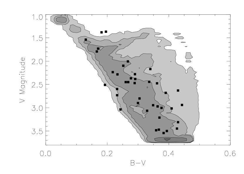
Figure 5.— A model of the blue stragglers in the core of 47 Tuc, starting collisions 7 Gyr ago and ending them at the present day. This model uses a mass function of $-8$. The observed blue stragglers are represented by squares. The contour levels are at 0.1%, 0.5%, 1%, 5% and 10% of the total population. The models with blue straggler formation starting at earlier than 7 Gyr ago were all very similar to those shown here.

4.2. The Middle Region of Our Dataset

The $25^{\prime\prime}$ to $130^{\prime\prime}$ part of the cluster contains none of the brightest blue stragglers, but still has a significant population of moderately bright stars. This region has the smallest number of blue stragglers out of the three regions we have chosen. Partly this is due to the shape of the HST/WFPC2 chip, but it has also been shown that blue stragglers are less prevalent in this area of 47 Tuc (Ferraro et al., 2004). The middle region is clearly the transition between the other two areas, being bluer than the outer region, and fainter than the core. It is reasonable to expect that the time frame and mass function that fit this region will also be a transition between the other two. In this area, three stars cannot be accounted for by our simulations. These stars are the only blue stragglers in the entire cluster that appear to the left of all of our simulated tracks in the colour-magnitude diagram. These three stars are shown as open circles in Figure 4, and are not included in our analysis of this region. They are discussed in further detail in the Summary & Discussion section.

In varying the collision time frame for this region, we found that by stopping the blue straggler formation process 0.6 Gyr ago, we were able to most closely approximate the blue straggler distribution in the colour-magnitude diagram. We then varied the mass function for this and similar timeframes, and found that the data is most accurately represented using a mass function with slope -3.

Using this mass function and starting the collision process 7 Gyr ago, we achieve the closest fit of 51% probability that the data and model were drawn from the same distribution, while starting it 8 Gyr ago gives a similar fit of 49%. A start time of 6 Gyr also works reasonably well, at 44%, but start times before or after these three drop in effectiveness. The colour-magnitude diagram of the best-fit model is given in Figure 6. If we include the three bluest stars in our analysis, the KS probability for the best-fit model drops to 27%. These stars are discussed in detail in section 6.

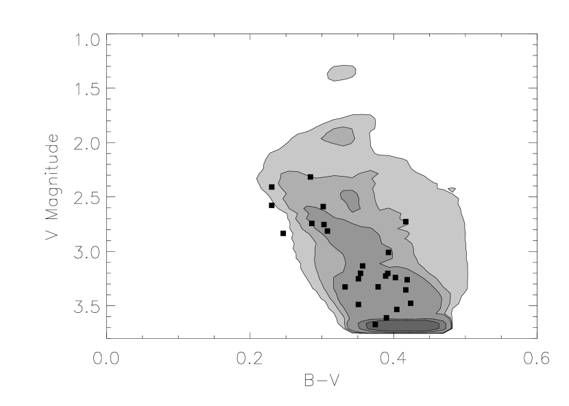
Figure 6.— The colour-magnitude diagram of models of blue stragglers just outside the core of 47 Tuc. The model starts collisions 7 Gyr ago, ends them 0.6 Gyr ago, and uses a mass function slope of -3. The observed blue stragglers are represented by squares, and the contour levels are the same as for Figure 5.

4.3. The Outermost Region

The outer region of the cluster, between $130^{\prime\prime}$ and $1200^{\prime\prime}$ from the cluster centre, contains a less diverse population than the other two areas. As can be seen in Figure 4, all of the stars in this region are in the same group in the colour-magnitude diagram. The colour of these stars suggests that they are older and less massive than the other blue straggler populations. There is a dense group of the coolest stars whose density is never accounted for by our simulations. Our evolutionary tracks travel quickly through this region, and so we predict a smaller number of blue stragglers than we observe. We analyze this region with and without these 9 coolest stars, to ensure that they do not mask any results for the rest of the region. We discuss these 9 blue stragglers in further detail in the Summary & Discussion section.

We find that, whether we include the coolest stars or not, our simulations best fit the data when we stop the collision process 1.2 Gyr ago. We adjust the start times of this process, and see that the data is most accurately represented by a collision process that starts between 9 and 7 Gyr ago. We are most successful at representing this data when using a mass function with a slope of +1.35, the Salpeter value. This supports a bias toward more low-mass stars in this part of the cluster.

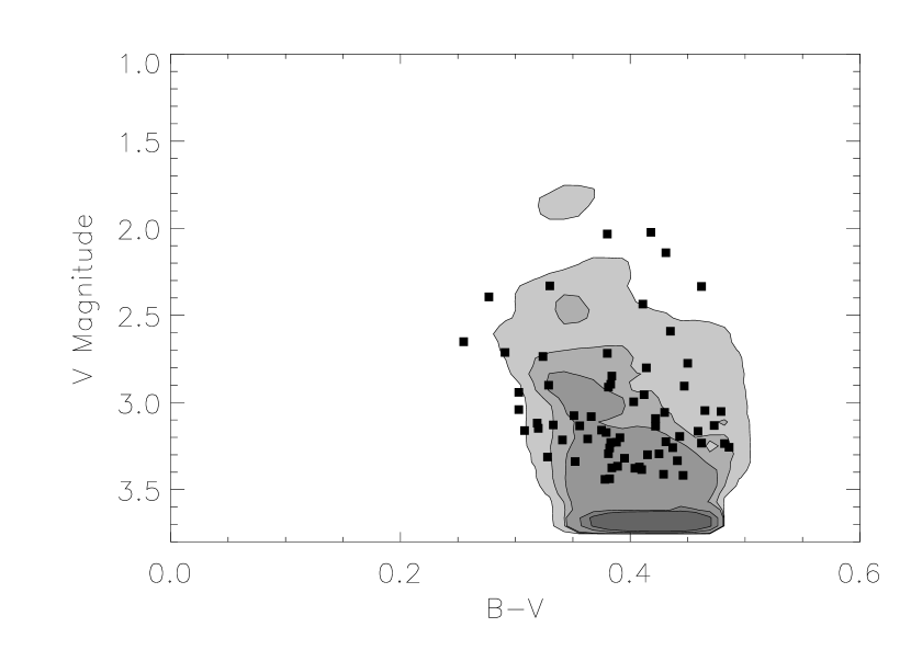
Figure 7.— Model of the blue stragglers that are farthest from the cluster centre. Observed blue stragglers are represented by squares, and the contour levels are the same as for Figure 5. All shown models use a mass function with slope of +1.35, start collisions 7 Gyr ago, and end collisions 1.2 Gyr ago.

When including the coolest stars in this area, we are not able to produce convincing models of the data. We achieve our most accurate model by starting the collision process 7 Gyr ago, producing a model that matches the data to 17%. When not including the coolest stars, our models are much better at fitting the data. We use a collision start time of 7 Gyr, with an end time of 1.2 Gyr, and find that this models the data to within 35%. Our best model can be seen in Figure 7.

These results indicate that the blue straggler population at the edge of 47 Tuc is much older than in the rest of the cluster. We see that the production of these blue stragglers must have begun around the same time as in the rest of the cluster, but has stopped earlier. As we are unable to accurately reproduce the data in the outermost region of 47 Tuc using only the collision mechanism, our simulations support binary mergers and mass accretions as being the dominant forms of blue straggler formation in the outskirts of this cluster, in agreement with Mapelli et al. (2004). These formation mechanisms would produce distributions in the colour-magnitude diagram that are somewhat similar to those produced through collisions, and so the small agreement between our simulations and the data would be expected in this case.

The basic problem with our models for this region of the cluster is that the collision models and the assumptions we have made about the dynamical state of the cluster do not accurately reproduce the balance of faint and bright blue stragglers. We can find models that match the brighter blue stragglers, but if we do, then we predict far too many faint blue stragglers. Any mechanism that is at work in the outskirts of the cluster must produce a more uniform distribution of blue stragglers in luminosity than the collision models used here.

5. Mass Segregation in the Core of 47 Tucanae

The collisional model used to interpret our blue straggler data predicts a mass function that is strongly weighted towards massive stars at the centre of the cluster, and should become less top heavy as one moves to the outskirts of the cluster. Next we compare these model predictions to the stellar mass function derived by comparing the observed luminosity function in a succession of radial bins in the central region of 47 Tuc to theoretical ones obtained from isochrones based on a range of power-law mass functions (Bergbusch & VandenBerg, 2001). The depth and improved resolution of the ultra-deep data set result in complete photometry fainter than $M_{V}=+8$ at all radii and are therefore well suited for the measurement of the mass function. The details of the derivation of stellar mass function as a function of radius in 47 Tuc are given in the companion paper by Guhathakurta et al. (2006).

Figure 8.— The power-law mass function exponent $x$ in a series of radial bins. Circles represent bins on the PC CCD, while squares are on the WF CCDs. Open points are from the archival data set, while solid points are from the ultra-deep data set. The open triangle is the inner most radial bin on the WF CCDs of the archival data set, which is most affected by stellar crowding.

As shown in Figure 8, the stellar mass function slope in 47 Tuc increases from $x=-5$ in the innermost bin to $x\sim-1$ in the outermost radial bins. It should be noted that Pryor, Smith, & McClure (1986) predict mass function slopes increasing from $x=-3$ to $x\sim 0$ over the same range in radius in the most centrally concentrated King models considered. Thus, the extremely negative mass function in the core of 47 Tuc determined directly from the observations ($x\sim-5$) agrees reasonably well with the value determined from the blue straggler models ($x\sim-8$), and with dynamical predictions of mass segregation. Given the uncertainties and simplifying assumptions inherent in the blue straggler models, we argue that these two values are in good agreement. The true mass function in the core may not actually be as steep as $x=-8$, but two independent measures tell us that it cannot be much flatter, and it certainly is not anything like a Salpeter or other normal initial mass function. Our blue stragglers models with a mass function of $x=-5$ fit the observations in the inner region at the 67% level, which is pretty good. We should also note that the blue straggler models for the 25” to 130” region of the cluster also favour a mass function that agrees with the observed value of $x\sim-3$.

6. Summary & Discussion

We found that, using the collision mechanism for blue straggler formation, we were able to reproduce the observed distribution of blue stragglers in colour-magnitude diagrams, to varying precision in different areas of 47 Tuc. We used simulations to find the time over which these stars were produced, along with the mass function of the progenitor stars. We separated our data on blue stragglers by dividing the stars into three groups, categorized by radial distance from the cluster centre, and reproduced each group separately.

In our outermost region, extending from $130^{\prime\prime}$ to $1200^{\prime\prime}$ from the cluster centre, our models matched the data to a maximum accuracy of 35%. In order to achieve this match, our simulations began the formation of blue stragglers between 7 and 9 Gyr ago, and ended it 1.2 Gyr ago. We found that using a mass function index of +1.35, the Salpeter value, produced the closest fit to the data. The middle region of 47 Tuc, $25^{\prime\prime}$ to $130^{\prime\prime}$ from the cluster centre, had a younger population of blue stragglers than this outermost area. We found that by starting stellar collisions between 6 and 8 Gyr ago, and ending them 0.6 Gyr ago, we could reproduce the data to a higher degree of certainty than for the outer region. A mass function with slope of -3 most accurately represented our data, giving a 50% probability that the data and model were drawn from the same distribution. We rediscovered the cluster core, with a $25^{\prime\prime}$ radius, based on the blue straggler photometric information alone. We started the blue straggler formation at various times, from the birth of the cluster to 8 Gyr ago, and let it continue until now. We found that a mass function slope of -8 allowed us to reproduce our data with an over 90% certainty.

In the outermost region of 47 Tuc, a group of the 9 coolest blue stragglers were not well-represented by any of our simulations. To ensure that these stars alone were not interfering with our results, we analyzed the region with and without including them. In both cases it was found that we were unable to account for the outermost population of blue stragglers using only the collision mechanism, but the nature of these 9 stars is still unknown. If they are collisional in origin, then they would have to be the result of a very rapid burst in formation. If there was a burst of collisions at the correct time, involving stars of a particular mass, then all those stars would be at the same place on their evolutionary track, producing the observed enhancement in that particular region of the colour-magnitude diagram. This scenario is extremely unlikely. A better solution is probably that these stars are not collisional in origin, and it is then outside of the scope of this paper to predict how and when these blue stragglers were produced, although we can say that they must be relatively old. Given their location in the Hertzsprung gap, other scenarios must be considered as well, such as whether these stars are actually blends, either real (i.e. binary systems) or due to observational error. Such blue stragglers have been found in almost every other globular cluster that has been observed carefully.

In the middle region of our dataset, three blue stragglers were not included in our analysis. These three stars were hotter than any of our evolutionary tracks at their respective luminosities, and so our simulations were incapable of reproducing them. These stars were the only ones in the cluster that had this difficulty, which indicates that they are different in origin from the other blue stragglers, and are almost certainly not collisional. The existence of these strange blue stragglers lends further support to our conclusion that the blue stragglers in this area of the cluster are not entirely collisional in origin. What is needed now is evolutionary tracks of binary merger products, so that the same kind of simulations as presented in this paper can be done with a different model for blue straggler evolution. These models have been completely lacking in the past; we look with interest to the preliminary models presented by Tian et al. (2006).

Both sets of blue stragglers that are not well-represented by our models lie reasonably close to the boundaries of our models. It is possible that photometric errors are responsible for the seeming disagreement with the models. However, in order for that to be the case, the photometric errors on these stars must be high, and the errors must be biased so as to move all the stars towards the models. We find it unlikely that such a fortunate coincidence has occurred.

While there has almost certainly been some rate of stellar collisions throughout the life of 47 Tuc, we have shown that the majority of these collisions have been occuring since early in the life of the cluster, but outside of the core the collision rate has substantially dropped within the past few hundred million years. We found that the regions that are farthest from the core have not had a significant collision rate for the longest amount of time, and that as we look closer to the centre, we see more and more evidence of recent collisions. We showed that the farthest region of 47 Tuc has probably not had a high rate of blue straggler formation for over the past $\approx$1 Gyr, and that the region close to the core has not been producing many blue stragglers for about half as long. The distributions depend much less on the start times than on the end times, so we were unable to isolate specific start times for our collisions. When the older stars evolve over such a large period of time, most of them become white dwarfs and leave the observable range of objects. These stars will then have no bearing on the final distribution of blue stragglers, and so the majority of the stars produced from an earlier start time do not affect our results. The end times that we found are reasonable, as one would expect stellar collisions to still be a significant part of the dynamics in the very dense core of a globular cluster. It also seems reasonable that in the further out regions, where densities are very low, there would not be a very high rate of blue straggler production.

We showed that the stars involved in blue straggler formation in the outermost region of 47 Tuc were described by a mass function with slope +1.35. This mass function favours lower mass stars over higher mass ones, and indicates that in the outer region, where one would expect the mass function of all the stars to have a value similar to this, the blue stragglers are formed approximately equally by all masses of stars. This result was echoed in our findings for the intermediate region, where it was shown that a mass function index of $-3$ produced the best fit to the data. In §5 we showed that the mass function near the outer edge of this region is $-2$, and then rises to $-5$ in the centre of the core. The mass function of $-3$ is an intermediate value in this region, and indicates that, like in the outer region, the distribution of masses in the blue straggler progenitors are representative of the overall stellar mass distribution.

In the core of 47 Tuc, we found that a mass function slope of $-8$ fit best with our data. This low mass function index was partially caused by our simulation, which assumed that all stars in the cluster were traveling at the same velocity of 11 km s^-1. If the stars in the core of 47 Tuc all had similar kinetic energies, as they are expected to through energy equipartition, then the square of their speeds would be inversely proportional to their masses, and the more massive stars will be moving slower than the less massive ones. The gravitational cross section for a stellar collision is inversely proportional to the relative velocity between the colliding stars, and so a collision involving a slower moving star should have a larger gravitational cross section than a collision involving faster moving stars. This increase in the gravitationally focused cross section will raise the collision rate for higher mass stars, beyond that which we took account of. In order to compensate for this, our simulation has to use a mass function that is more heavily weighted toward massive stars than is actually be present, and so the very steep mass function that we found is, in part, caused by our simulation’s assumption of constant stellar speed. This result is most noticeable in the core of the cluster due to the much higher concentration of high mass stars. Even with this effect, however, the progenitors of the blue stragglers in the core of 47 Tuc were still significantly more massive than in the rest of the cluster. The simulations we ran are not able to account for this effect directly by changing the velocities of the individual stars. However, if we simply reduce the velocity dispersion in the cluster by a factor of 2 (to 5 km s^-1) and perform our simulations again, we find that our best fit scenario still has a mass function of $x=-8$, but that it is only slightly better than the same simultion with $x=-5$. It is also apparent the more massive blue stragglers are slightly better fit with the higher mass function index. that Therefore, we conclude that our mass function index derived from the blue stragglers is indeed biased towards very low values.

We found that it was much easier to replicate the distribution of blue stragglers in the core than in the rest of the cluster. This suggests that the blue stragglers in the core may be formed almost entirely through stellar collisions. The number of collisions rapidly increases with increasing density, and so, in the core of the cluster, where densities are orders of magnitudes larger than in the outer regions, stellar collisions should be a much more dominant effect. The rest of the cluster should be less effected by collisions, and our results show that outside of a few core radii, stellar collisions are much less influential on the blue straggler distribution than other formation mechanisms. This is in agreement with the predictions of collision probability in the outskirts of the cluster.

The models of blue straggler formation in the core of the cluster suggest that the mass function is strongly weighted towards massive stars, and the HST results confirm this for the present day. However, the fact that all blue stragglers in the core require a strongly negative mass function suggests that the mass function has been this unusual for at least the lifetime of the brightest blue stragglers, on the order of a few hundred million years. Interestingly, the timescale for energy equipartition for most globular clusters is also on the order of $10^{8}$ years. It may be that detailed studies of the cores of other globular clusters will also show this extreme mass function. If this is the case, we would expect that the luminosity function of blue stragglers in the cores of clusters should extend to brighter (i.e. more massive) stars than the luminosity function in the outskirts of the cluster.

Blue stragglers are touted as tracers of dynamics in globular clusters (Hut, 1993; Sills & Bailyn, 1999) since they are thought to form during stellar encounters. Recent results from Piotto et al. (2004) have brought this claim into question, since they find no correlation between blue straggler populations and the expected collision rate in the cluster. In this paper, we have shown that using the blue stragglers alone, we can discover the core radius of 47 Tuc at least as well as traditional methods. Or, to say it more accurately, the blue stragglers inside and outside the core radius are drawn from clearly different populations. We have also shown that we can find evidence of mass segregation by applying a very simplistic model of blue straggler formation to the blue straggler populations in different regions of the cluster. Therefore, blue stragglers must have some connection to globular cluster dynamics. The simple picture of blue straggler formation (i.e. stellar collisions in globular clusters, merger of primordial binaries in other environments) is too simplistic, but this interesting population can still be used to study globular clusters in their entirety.

In all regions of 47 Tuc, blue stragglers started forming at very early times in the cluster – at least 7 Gyr ago, although our data are not sufficient to probe further back than that. However, in the outskirts of the cluster, formation of bright blue stragglers ended before it ended in the core. There are two possible reasons for this (both of which could be operating). Either, bright blue stragglers can only be formed in collisions, or the populations of binary stars are different inside and outside the core. Collisions are the only way to produce blue stragglers with masses significantly greater than twice the turnoff mass, and therefore it may be reasonable to suggest that the brightest blue stragglers are, in fact, triple collisions. If the binary population inside the core consisted of a large number of massive, hard binaries, then encounters between these binary systems would result in more triple collisions than the encounters outside the core. Binaries in the outskirts of the cluster would have to be either less massive or consist of only wide binaries that could not merge in the cluster lifetime. Is it possible that all the blue-straggler-producing binaries could have migrated into the core during the cluster lifetime? Or that binaries in the core are made to be more massive through dynamical interactions (Davies et al., 2004)? The timescales for mass segregation discussed above suggest that this is likely, and the dynamical models of Mapelli et al. (2004) are in agreement as well (although in their model, some fraction of the binaries that can produce blue straggler remain outside the core and produce the peripheral blue stragglers). In both the Mapelli and Davies models, blue stragglers were given a finite lifetime, but their position in the colour-magnitude diagram was not considered. An obvious next step would be to combine such models with blue straggler evolutionary tracks, as an improvement over the simple models presented in this paper.

There are an increasing number of recent studies of blue stragglers in globular clusters that are combining ground-based wide-field data with high quality HST data for the cores of clusters (Ferraro et al., 2004; Sabbi et al., 2004). The same kinds of models can be, and should be, created for these clusters. We have very interesting indications that something dynamical is happening to the blue straggler populations in clusters with the evidence that the ‘unusual’ bimodal population of blue stragglers in M3 is not unusual at all, but seen in at least four other clusters (47 Tuc, M55 and NGC 6752; see Ferraro, 2006) and (M5; see Warren, Sandquist & Bolte, 2006)). What does the distribution of blue stragglers in the colour-magnitude diagram look like in the different regions of these clusters? And how can we explain these results? We suggest that blue stragglers do trace the dynamical state and history of their parent globular clusters, and that their secrets can be unlocked through detailed and consistent studies of their populations in a variety of clusters.

References

- Albrow et al. (2001) Albrow, M. D., Gilliland, R. L., Brown, T. M., Edmonds, P. D., Guhathakurta, P., & Sarajedini, A. 2001, ApJ, 559, 1060
- Bergbusch & VandenBerg (2001) Bergbusch, P. A., & VandenBerg, D. A. 2001, ApJ, 556, 322
- Davies et al. (2004) Davies, M. B., Piotto, G., & De Angeli, F. 2004, MNRAS, 349, 129
- De Marco et al. (2005) De Marco, O., Shara, M. M., Zurek, D., Ouellette, J. A., Lanz, T., Saffer, R. A., & Sepinsky, J. F. 2005, ApJ, 632, 894
- Ferraro et al. (2001) Ferraro, F. R., D’Amico, N., Possenti, A., Mignani, R. P., & Paltrinieri, B. 2001, ApJ, 561, 337
- Ferraro et al. (2004) Ferraro, F. R., Beccari, G., Rood, R. T., Bellazzini, M., Sills, A., & Sabbi, E. 2004, ApJ, 603, 127
- Ferraro (2006) Ferraro, F. R. 2006, ASP Conf. Ser. TBA, Resolved Stellar Populations (astro-ph/0601217)
- Gebhardt et al. (1995) Gebhardt, K., Pryor, C., Williams, T. B., & Hesser, J. E. 1995, AJ, 110, 1686
- Gilliland et al. (2000) Gilliland, R. L., et al. 2000, ApJ, 545, L47
- Gratton et al. (2003) Gratton, R. G., Bragaglia, A., Carretta, E., Clementini, G., Desidera, S., Grundahl, F., & Lucatello, S. 2003, A&A, 408, 529
- Guenther et al. (1992) Guenther, D. B., Demarque, P., Kim, Y.-C., & Pinsonneault, M. H. 1992, ApJ, 387, 372
- Guhathakurta et al. (2006) Guhathakurta, P., Howell, J. H., Clem, J. L., Gilliland, R. L., & Sills, A. 2006, ApJ, submitted (astro-ph/0605XXX)
- Howell et al. (2000) Howell, J. H., Guhathakurta, P., & Gilliland, R. L. 2000, PASP, 112, 1200
- Hut (1993) Hut, P. 1993, ASP Conf. Ser. 53: Blue Stragglers, 53, 44
- Leonard (1989) Leonard, P. J. T. 1989, AJ, 98, 217
- Leonard & Linnell (1992) Leonard, P. J. T., & Linnell, A. P. 1992, AJ, 103, 1928
- Mapelli et al. (2004) Mapelli, M., Sigurdsson, S., Colpi, M., Ferraro, F. R., Possenti, A., Rood, R. T., Sills, A., & Beccari, G. 2004, ApJ, 605, L29
- McCrea (1964) McCrea, W. H. 1964, MNRAS, 128, 147
- McMillan & Hut (1996) McMillan, S. L. W., & Hut, P. 1996, ApJ, 467, 348
- Piotto et al. (2002) Piotto, G., King, I. R., Djorgovski, S. G., Sosin, C., Zoccali, M., Saviane, I., De Angeli, F., Riello, M., Recio- Blanco, A., Rich, R. M., Meylan, G., & Renzini, A. 2002, A&A, 391, 945
- Piotto et al. (2004) Piotto, G., De Angeli, F., King, I. R., Djorgovski, S. G., Bono, G., Cassisi, S., Meylan, G., Recio-Blanco, A., Rich, R. M., & Davies, M. B. 2004, ApJ, 604, L109
- Pryor et al. (1986) Pryor, C., Smith, G. H., & McClure, R. D. 1986, AJ, 92, 1358
- Sabbi et al. (2004) Sabbi, E., Ferraro, F. R., Sills, A., & Rood, R. T. 2004, ApJ, 617, 1296
- Sills & Bailyn (1999) Sills, A., & Bailyn, C. D. 1999, ApJ, 513, 428
- Sills & Lombardi (1997) Sills, A., & Lombardi, J. C., Jr. 1997, ApJ, 484, L51
- Sills et al. (2000) Sills, A., Bailyn, C. D., Edmonds, P. D., & Gilliland, R. L. 2000, ApJ, 535, 298
- Stetson (1992) Stetson, P. B. 1992, ASP Conf. Ser. 25: Astronomical Data Analysis Software and Systems I, 25, 297
- Tian et al. (2006) Tian, B., Deng, L., Han, Z., Zhang, X. B. 2006 (astro-ph/0604290)
- Warren, Sandquist & Bolte (2006) Warren, S. R., Sandquist, E. L., & Bolte, M. 2006 (astro-ph/0605047)
- Zinn & Searle (1976) Zinn, R., & Searle, L. 1976, ApJ, 209, 734