Calcium II Triplet Spectroscopy of LMC Red Giants. I. Abundances and Velocities for a Sample of Populous Clusters

Abstract

Utilizing the FORS2 instrument on the Very Large Telescope, we have obtained near infrared spectra for more than 200 stars in 28 populous LMC clusters. This cluster sample spans a large range of ages ($\sim$ 1$-$13 Gyr) and metallicities ($-0.3\mathrel{>\kern-10.00002pt\lower 3.87495pt\hbox{$\sim$}}$ [Fe/H] $\mathrel{>\kern-10.00002pt\lower 3.87495pt\hbox{$\sim$}}-2.0$) and has good areal coverage of the LMC disk. The strong absorption lines of the Calcium II triplet are used to derive cluster radial velocities and abundances. We determine mean cluster velocities to typically 1.6 km s^-1 and mean metallicities to 0.04 dex (random error). For eight of these clusters, we report the first spectroscopically determined metallicities based on individual cluster stars, and six of these eight have no published radial velocity measurements. Combining our data with archival HST/WFPC2 photometry, we find the newly measured cluster, NGC 1718, is one of the most metal-poor ([Fe/H] $\sim$ $-$0.80), intermediate age ($\sim$ 2 Gyr) inner disk clusters in the LMC. Similar to what was found by previous authors, this cluster sample has radial velocities consistent with that of a single rotating disk system, with no indication that the newly reported clusters exhibit halo kinematics. Additionally, our findings confirm previous results which show that the LMC lacks the metallicity gradient typically seen in non-barred spiral galaxies, suggesting that the bar is driving the mixing of stellar populations in the LMC. However, in contrast to previous work, we find that the higher metallicity clusters ($\mathrel{>\kern-10.00002pt\lower 3.87495pt\hbox{$\sim$}}-1.0$ dex) in our sample show a very tight distribution (mean [Fe/H] = $-0.48$, $\sigma$ = 0.09), with no tail toward solar metallicities. The cluster distribution is similar to what has been found for red giant stars in the bar, which indicates that the bar and the intermediate age clusters have similar star formation histories. This is in good agreement with recent theoretical models that suggest the bar and intermediate age clusters formed as a result of a close encounter with the SMC $\sim$ 4 Gyr ago.

1 Introduction

In the current paradigm of galaxy formation, it is believed that the formation history of spiral galaxy spheroids, such as the Milky Way (MW) halo and bulge, may be dominated by the accretion/merger of smaller, satellite galaxies (e.g. Searle & Zinn 1978, Zentner & Bullock 2003). This type of galactic interaction is currently seen in the Sagittarius Dwarf galaxy (Sgr), which is in the midst of being cannibalized by the MW. However, due to its location on the opposite side of the Galaxy from us (Ibata, Gilmore, & Irwin 1994), contamination by MW foreground stars makes it difficult to study stellar populations in Sgr. In contrast, both the Large Magellanic Cloud (LMC) and Small Magellanic Cloud (SMC), two satellite galaxies which may eventually be consumed into the MW halo, suffer little from foreground contamination due to their direction on the sky, which places them well out of the plane of the MW. Additionally, the relative proximity of these galaxies allows us to easily resolve stellar populations in the Magellanic Clouds down below their oldest main sequence turnoffs (MSTOs). Thus, the LMC and SMC offer us a golden opportunity to study the effects of dynamical interactions on the formation and evolution of satellite galaxies; this information plays an integral part in discovering the secrets of spiral galaxy formation.

One of the most direct ways to determine the chemical evolution (CEH) and star formation history (SFH) of a galaxy is through the study of its star clusters, which preserve a record of their host galaxy’s chemical abundances at the time of their formation. The LMC star clusters continue to play a critical role in shaping our understanding of the age-metallicity relation of irregular galaxies. The rich star cluster system of the LMC is also a unique resource for many experiments in stellar and galactic astronomy, largely due to the fact that the LMC harbors well populated clusters that occupy regions of the age-metallicity plane that are devoid of MW clusters. Thus, LMC clusters have been widely studied as a test of stellar evolution models at intermediate metallicity and age (e.g., Bertelli et al. 2003; Brocato, Castellani & Piersimoni 1994; Ferraro et al. 1995) and as empirical templates of simple stellar populations for applications to population synthesis models of unresolved galaxies (e.g., Beasley, Hoyle & Sharples 2002; Leonardi & Rose 2003; Maraston 2005).

The LMC cluster system, however, is well known to show a puzzling age distribution, with a handful of old ($\sim$ 13 Gyr), metal-poor globular clusters, a number of intermediate age (1$-$3 Gyr), relatively metal-rich populous clusters and apparently only one cluster, ESO 121-SC03 ($\sim$ 9 Gyr, hereafter ESO 121), that falls into the LMC’s so-called ‘age gap’ (e.g. Da Costa 1991; Geisler et al. 1997; Da Costa 2002). We note that the LMC bar seems to show a formation history very similar to that of the clusters (Cole et al. 2005), while field SFHs derived from deep color-magnitude diagrams (CMDs) suggest that stars in the LMC disk had a constant, albeit low, star formation rate during the cluster ‘age-gap’ (e.g. Holtzmann et al. 1999, Smecker-Hane et al. 2002). While the cause of the cessation of cluster formation (the beginning of the age gap) is not known, dynamical simulations by Bekki et al. (2004) suggest that the recent burst of cluster formation is linked to the first very close encounter between the Clouds about 4 Gyr ago, which would have induced “dramatic gas cloud collisions”, allowing the LMC to begin a new epoch of cluster and star formation; strong tidal interactions between the Clouds have likely sustained the enhanced cluster formation. Bekki et al. (2004) also find that the close encounter between the clouds would have been sufficient to cause the formation of the LMC bar around the time of the new epoch of cluster formation, giving rise to the similar SFHs seen in the cluster system and the bar. In addition to enhancing star formation, tidal forces can result in the infall or outflow of material, thereby affecting the CEH of the LMC and, at the same time, leaving behind a signature of the interaction. Thus, accurate knowledge of the ages and metallicities of LMC clusters is necessary to fully understand the formation and dynamical history of this galaxy.

While age and metallicity estimates from isochrone fitting to CMDs exist for a large number of clusters, the degeneracy between age and metallicity make these estimates inherently uncertain in the absence of solid metallicity measurements based on spectroscopic data. Integrated light has been used to measure [Fe/H] for many of these clusters, however, these values are often problematic since the cluster light can be dominated by a few luminous stars, and the results are susceptible to small-number statistical effects. In recent years, high spectral resolution studies of a few prominent clusters have been undertaken, yielding, for the first time, detailed abundance estimates of a wide variety of elements, including iron, for individual stars within these clusters (Hill 2004; Johnson et al. 2006). This work is highly valuable, but because of the large investment in telescope time necessary to obtain data of sufficiently high signal-to-noise (S/N) ratio, it has necessarily been limited to only a few stars in a few clusters; most of these targets are very old, leaving the vast majority of young and intermediate age clusters unmeasured.

Moderate resolution studies are an excellent complement to high resolution work for a couple of reasons. First, the multi-object capability available for many moderate resolution spectrographs makes it possible to observe many potential cluster members in a given field. This increases the probability of observing true cluster members, and facilitates their identification, even in sparse clusters. Second, less integration time is needed to achieve the desired S/N ratio at moderate resolution, allowing the observation of many more targets in a given amount of time. Thus, with moderate resolution spectra we can observe a large number of targets in a short period of time and thereby create an overview of a galaxy’s global metallicity distribution, both spatial and temporal. This approach is particularly important for the LMC since its metallicity distribution is very broad and the intrinsic shape is not very well known.

To date, the only large-scale spectroscopic metallicity determination for LMC clusters based on individual cluster stars has been the landmark study by Olszewski et al. (1991, hereafter OSSH; Suntzeff et al. 1992). They obtained medium-resolution spectra of red giant branch (RGB) stars in $\sim$ 80 clusters at a wavelength of $\approx$ 8600 Å, centered on the very prominent triplet of calcium II (CaT) lines. Their work was motivated by the recognition that the CaT lines were proving to be a reliable metallicity indicator for Galactic globular clusters (e.g., Armandroff & Zinn 1988; Armandroff & Da Costa 1991). Additionally, this spectral feature is easily measured in distant targets and at medium resolution since the CaT lines are extremely strong and RGB stars are near their brightest in the near-infrared. Using the CaT, OSSH calculated metallicities and radial velocities for 72 of their target clusters. Analysis of the metallicity distribution showed that the mean [Fe/H] values for all clusters in the inner (radius $<$ 5$\arcdeg$) and outer (radius $>$ 5$\arcdeg$) LMC are almost identical ($-0.29\pm 0.2$ and $-0.42\pm 0.2$, respectively), suggesting the presence of little if any radial metallicity gradient, in sharp contrast to what is seen in the MW (e.g. Friel et al. 2002) and M33 (Tiede, Sarajedini, & Barker 2004). Using radial velocities from the OSSH sample, Schommer et al. (1992) found that the LMC cluster system rotates as a disk, with no indication that any of the clusters have kinematics consistent with that of a pressure supported halo.

However, the results of OSSH present some difficulties owing to limitations of technology at the time. The use of a single-slit spectrograph severely limited the number of targets observed toward each cluster. Additionally, the distance of the LMC paired with a 4m telescope required that they observe the brightest stars in the clusters. Many of these stars are M giants, which have spectra contaminated by TiO (although it may not be significant until spectral type M5 or later), or are carbon stars, neither of which are suitable for using the CaT to determine [Fe/H]. Thus, the combination of a single-slit spectrograph with a midsized telescope made it difficult for OSSH to build up the number of target stars necessary to differentiate between cluster members and field stars. Most of the resulting cluster values are based on only one or two stars; in some cases, there are metallicity or radial velocity discrepancies between the few stars measured, and it is unclear which of the values to rely on.

The interpretation of the OSSH results is further complicated by subsequent advances both in knowledge of the globular cluster metallicity scale to which the CaT strengths are referred (Rutledge et al. 1997b) and in the standard procedure used to remove gravity and temperature dependencies from the CaT equivalent widths (Rutledge et al. 1997a). It is not a simple matter to rederive abundances from the equivalent widths of OSSH because of the lack of homogeneous photometry for many of the clusters; mapping the OSSH abundances to a modern abundance scale (e.g., that defined at the metal-poor end by Carretta & Gratton 1997 and near solar metallicity by Friel et al. 2002) is insufficient because the transformation is nonlinear and random metallicity errors tend to be greatly magnified (see Cole et al. 2005).

In an effort to produce a modern and reliable catalog of LMC cluster metallicities, we have obtained near-infrared spectra of an average of eight stars in each of 28 LMC clusters. We have taken advantage of the multiplex capability and extraordinary image quality and light-gathering power of the European Southern Observatory’s 8.2m Very Large Telescope, and of the great strides in the interpretation and calibration of Ca II triplet spectroscopy made in the past 15 years to provide accurate cluster abundances with mean random errors of 0.04 dex. Here we present our derived cluster metallicities and radial velocities and compare these results to previously published spectroscopic metallicities. The metallicity distribution of several hundred non-cluster LMC field stars will be presented in a forthcoming paper (Cole et al., in preparation). The current paper is laid out as follows: Section 2 discusses the observations and data processing. In §3 we present the derived cluster properties and comparisons to previous works are detailed in §4. Finally, in §5 we summarize our results.

2 Data

2.1 Target Selection

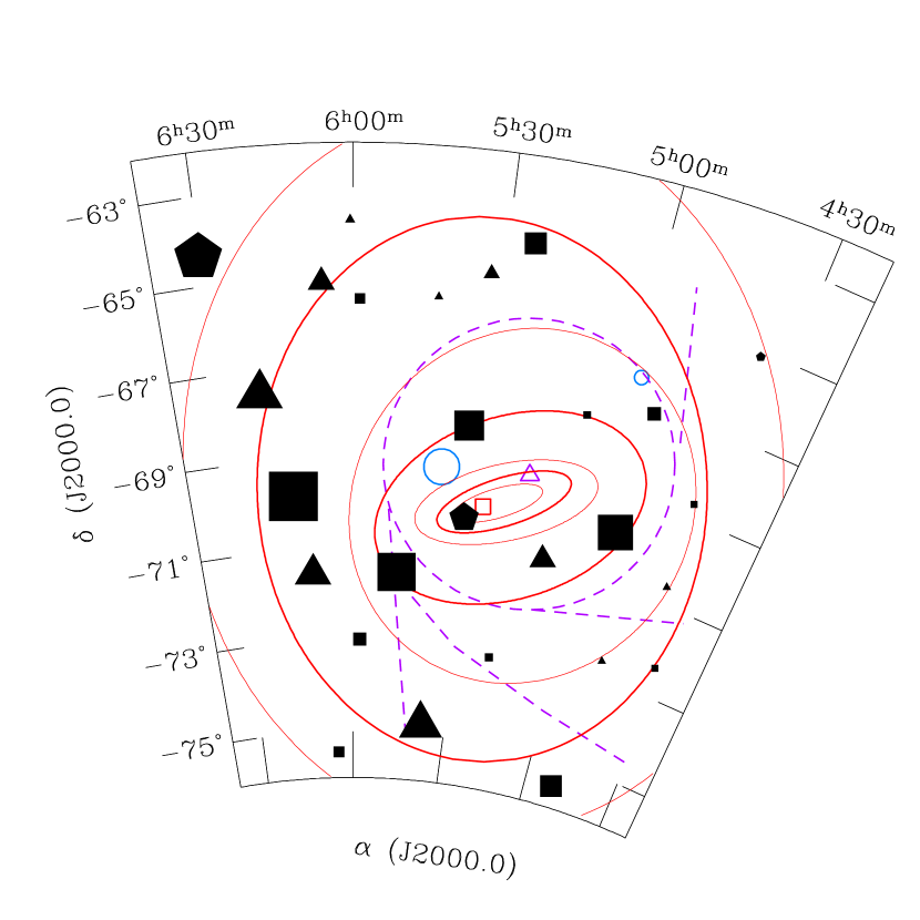
Figure 1: Diagram of the LMC showing the location of our target clusters along with prominent features in the LMC. Filled symbols represent the target clusters with symbol size directly related to V magnitude and shape denoting SWB Type, where the triangles, squares and pentagons are Type V, VI, and VII, respectively. Note that NGC 1841 (declination $\sim-84\arcdeg$) is outside of the range of this plot and NGC 1861 (SWB Type IVB) is marked as a solid triangle. Near IR isopleths from van der Marel (2001) are marked as solid lines while the dashed lines outline major H I features (see Staveley-Smith et al. 2003). The H I rotation center (Kim et al. 1998) is marked with the open triangle and the rotation center of the intermediate age stars (van der Marel et al. 2002) is shown by the open square. Finally, the two largest H II regions are marked as open circles.

We observed 28 prominent star clusters scattered across the face of the LMC, in environments ranging from the dense central bar to the low-density regions near the tidal radius (a 29th cluster was observed, however it appears to be too young to apply the CaT method; see appendix). Our observations were aimed at clusters rich enough and sufficiently large and diffuse to give us confidence in harvesting at least four definite cluster members from which to derive the cluster metallicity. In order to obtain leverage on the LMC age-metallicity relation, we included clusters from SWB class IVB$-$VII, spanning the age range of clusters containing bright, well-populated red giant branches (Persson et al. 1983; Ferraro et al. 1995). Our sample was intentionally biased towards those clusters with conflicting or uncertain previous abundance measurements, clusters thought to lie near the edge of the age gap, and those whose radial velocities might provide new insight into the dynamical history of the LMC-SMC system, based on their location. Our targets, their positions, sizes, integrated V magnitudes, and SWB types are listed in Table 1. A schematic of the LMC is presented in Fig. 1. Shown are near-infrared isopleths from van der Marel (2001; solid ellipses), at semi-major axis values of 1$\arcdeg$, 1$\fdg$5, 2$\arcdeg$, 3$\arcdeg$, 4$\arcdeg$, 6$\arcdeg$, and 8$\arcdeg$. Prominent H I features (dashed lines; Staveley-Smith et al. 2003), and the two largest centers of LMC star formation (30 Doradus and N11, open circles) are also plotted. Finally, the rotation center of intermediate age stars is denoted by the open square (van der Marel et al. 2002) and the H I rotation center from Kim et al. (1998) is plotted as the open triangle. Our target clusters are plotted with solid symbols, with the exception of NGC 1841, which lies farther south than the area covered by this diagram.

Pre-images of our target fields in $V$ and $I$ bands were taken by ESO Paranal staff in the fall of 2004, several months prior to our observing run. The pre-images were processed within IRAF, and stars were identified and photometered using the aperture photometry routines in DAOPHOT (Stetson 1987). Stars were cataloged using the FIND routine in DAOPHOT and photometered with an aperture size of 3 pixels. The $V$ and $I$ band data were matched to form colors. Red giant targets were chosen based on the instrumental CMD, and each candidate was visually inspected to ensure location within the cluster radius (judged by eye) and freedom from contamination by very nearby bright neighbors. In each cluster we looked for maximum packing of the $\approx 8\arcsec$-long slits into the cluster area and for the best possible coverage of the magnitude range from the horizontal branch/red clump ($V\approx$ 19.2) to the tip of the RGB ($V\approx$ 16.4). The positions of each target were defined on the astrometric system of the FORS2 pre-images so that the slits could be centered as accurately as possible, and the slit identifications were defined using the FORS Instrument Mask Simulator (FIMS) software provided by ESO; the slit masks were cut on Paranal by the FORS2 team.

2.2 Acquisition

The spectroscopic observations were carried out with FORS2, in visitor mode, at the Antu (VLT-UT1) 8.2m telescope at ESO’s Paranal Observatory, during the first half of the nights of 21-24 December 2004; weather conditions were very clear and stable during all 4 nights, with seeing typically 0.5$\arcsec$-1.0$\arcsec$. We used the FORS2 spectrograph in mask exchange unit (MXU) mode, with the 1028z+29 grism and OG590+32 order blocking filter. The MXU slit mask configuration allows the placement of more slits on the sky than the 19 movable slits provided in Multi Object Spectrograph mode. We used slits that were 1$\arcsec$ wide and 8$\arcsec$ long (7$\arcsec$ in a few cases) and, as mentioned above, targets were selected so as to maximize the number of likely cluster members observed; typically 10 stars inside our estimated cluster radius were observed, with an additional $\sim$ 20 stars outside of this radius that appeared to be LMC field red giants, based on our preimaging CMDs.

FORS2 utilizes a pair of 2k $\times$ 4k MIT/LL CCDs and the target clusters were centered on the upper (master) CCD, which has a readout noise of 2.9 electrons, while the lower (secondary) CCD, with a readout noise of 3.15 electrons, was used to observe field stars. The only exception to this was the Hodge 11/SL 869 field where, with a rotation of the instrument, we were able to center Hodge 11 in the master CCD and SL 869 in the secondary CCD. Both CCDs have an inverse gain of 0.7e^- ADU^-1. Pixels were binned 2$\times$2, yielding a plate scale of 0.25$\arcsec$ pixel^-1 and the resulting spectra cover 1750 Å, with a central wavelength of 8440 Å and a dispersion of $\sim$0.85 Å pixel^-1 (resolution of 2-3 Å). While the FORS2 field of view is 6.8$\arcmin$ across, it is limited to 4.8$\arcmin$ of usable width in the dispersion direction in order to keep important spectral features from falling off the ends of the CCD.

Each field was observed twice, with offsets of 2$\arcsec$ between exposures, to ameliorate the effects of cosmic rays, bad pixels and sky fringing. The total exposure time in each setup was either 2x300s, 2x500s or 2x600s. Both the readout time (26s) and setup time per field (some 6-10 minutes) were very quick and allowed us to obtain longer exposures than originally planned in many cases. For most of our targets with short exposure times (300s) we combined the spectra so as to improve the S/N ratio. However, with the longer exposures (500s and 600s) we found that the S/N ratio in a single exposure was adequate, and cosmic rays and bad pixels were not a problem, so we have used only one of the pair of exposures in our analysis. Column 8 of Table 1 gives the total exposure time that we have used in our analysis of each cluster.

Calibration exposures were taken in daytime, under the FORS2 Instrument Team’s standard calibration plan. These comprised lamp flat-field exposures with two different illumination configurations and He-Ne-Ar lamp exposures for each mask. Two lamp settings are required for the flat-fields because of parasitic light in the internal FORS2 calibration assembly.

In addition to the LMC clusters, we observed four Galactic stars clusters (47 Tuc, M 67, NGC 2298, and NGC 288), three of which are a subsample of the CaT calibration clusters in Cole et al. (2004; hereafter, C04). Since we used the same instrument setup as C04, we expected to use their CaT calibration, and these three clusters were observed to serve as a check on the validity of that approach. Processing of these three clusters shows that our results are identical to within the errors, thus we will use the CaT calibration of C04 rather than deriving our own CaT calibration coefficients.

2.3 Processing

Image processing was performed with a variety of tasks in IRAF. The IRAF task CCDPROC was used to fit and subtract the overscan region, trim the images, fix bad pixels, and flat field each image with the appropriate dome flats. The flat-fielded images were then corrected for distortions in order to facilitate extraction and dispersion correction of the spectra. The distortion correction is a two-step process, whereby first the image of each slitlet is rectified to a constant range of $y$-pixel (spatial direction) values on the CCD, and then the bright sky lines are traced along each slitlet and brought perpendicular to the dispersion direction. The amount of the distortion is minimal near the center of the field of view and increases toward the edges; in all cases it is fit with a polynomial that is at most quadratic in $y$ and linear in $x$. Although the distortion corrections are small, they greatly reduce the residuals left after sky subtraction and improve the precision and accuracy of the dispersion solution (see below).

Once distortion corrections were completed, the task APALL (in the HYDRA package) was used to define the sky background and extract the stellar spectra into one-dimension. The sky level was defined by performing a linear fit, across the dispersion direction, to sky ‘windows’ on each side of the star. This procedure presented few difficulties since the target stars were usually bright as compared to the sky and the seeing disks are small compared to the length of the slitlets. The only problems arose when the star fell near the top or bottom of the slitlet; in these cases the sky regions were chosen interactively and we found, for all of these spectra, that the resulting sky subtraction was indistinguishable from that of more centrally located stars. While daily arc lamp exposures are available for dispersion correcting the spectra, telescope flexure during the night, along with small slit centering errors, makes this a less desirable method for correcting the spectra. As such, greater than 30 OH night sky emission lines (Osterbrock & Martel 1992) were used by the IRAF tasks IDENTIFY, REFSPECTRA, and DISPCOR to calculate and apply the dispersion solution for each spectrum, which was found to be $\sim$ 0.85 Å pixel^-1 with a characteristic rms scatter of $\sim$ 0.06 Å. For the short (300s) exposure data, we processed both sets of images for each pointing and combined the dispersion corrected spectra using SCOMBINE to improve the S/N ratios for these stars. In a few cases we found that averaging the stellar spectra actually decreased the S/N ratio; for these stars we chose to use the higher quality of the two individual spectra in place of the averaged spectrum. All spectra were then continuum normalized by fitting a polynomial to the stellar continuum, excluding strong absorption features (both telluric and stellar). For the final spectra, S/N ratios are typically 25$-$50 pixel^-1 with some stars as high as $\sim$ 90 pixel^-1 and, in only a few cases, as low as $\sim$ 15 pixel^-1. Sample spectra showing the CaT region are presented in Fig. 2.

2.4 Radial Velocities

Accurate radial velocities for our target stars are important for two reasons. First and foremost, since a cluster’s velocity dispersion is expected to be relatively small compared to the surrounding field and its mean velocity quite possibly distinct from the field, radial velocities are an excellent tool for determining cluster membership. In addition, our equivalent width measuring program uses radial velocities to derive the expected CaT line centers.

Radial velocities for all target stars were determined through cross-correlation with 30 template stars using the IRAF task FXCOR (Tonry & Davis 1979) and we have chosen to use template spectra from C04. The template stars were observed as a part of their CaT calibration program, thus their sample offers a good match to the spectral types of our target stars. Additionally, their observations were made with a telescope and instrument setup that is almost identical to ours. C04 chose template stars for which reliable published radial velocity measurements were available. Template velocities come from the following sources: 11 stars from NGC 2298, NGC 1904, and NGC 4590 (Geisler et al. 1995), eight stars from Berkeley 20 and Berkeley 39 (Friel et al. 2002), two stars from Melotte 66 (Friel & Janes 1993), six stars from M67 (Mathieu et al. 1986), and three stars from 47 Tuc (Mayor et al. 1983). In addition to calculating relative radial velocities, FXCOR uses information about the observatory location and the date and time of the observations (once the ESO header has been appropriately reformatted) to correct the derived velocities to the heliocentric reference frame. For a star’s final heliocentric radial velocity, we adopt the average value of each cross-correlation result. We find good agreement amongst the template derived velocities, with a typical standard deviation of $\sim 6$ km s^-1 for each star.

When the stellar image is significantly smaller than the slit width, systematic errors due to imprecise alignment of the slit center and the stellar centroid can dominate the error budget in the radial velocity measurements. With the grism and CCD used here, an offset of one pixel across the four-pixel-wide slit would introduce an error in the measured velocity of $\approx 30$ km s^-1. We follow the approach of Tolstoy et al. (2001) in applying a correction to each measured radial velocity based on the individual slit offsets; following C04, we measure the slit offsets using acquisition (so-called “through-slit”) images taken immediately prior to the spectroscopic measurement, and estimate a precision of $\approx$0.14 pixels on the measured offset value. This introduces an error of $\pm$ 4.2 km s^-1 and, added in quadrature with the error resulting from the velocity cross-correlations, gives an error of roughly 7.5 km s^-1. We adopt this as the error in measuring the radial velocity of an individual star.

2.5 Equivalent Widths and Abundances

To measure the equivalent widths of the CaT lines, we have used a previously written fortran program (see C04 for details). However, since this region of a star’s spectrum can be contaminated by weak metal lines and, in some cases, weak molecular bands, measuring the true equivalent width of the CaT lines at all but the highest spectral resolutions is impossible. Instead, we follow the method of Armandroff & Zinn (1988) and define continuum bandpasses on either side of each CaT feature. In this wavelength range, the continuum slope of a red giant star is virtually flat, thus, the ‘pseudo-continuum’ for each CaT line is easily defined by a linear fit to the mean value in each pair of continuum windows. The ‘pseudo-equivalent’ width is then calculated by fitting the sum of a Gaussian and a Lorentzian, required to have a common line center, to each CaT line with respect to the ‘pseudo-continuum’. For reference, the rest wavelengths of the line and continuum bandpasses, as defined by Armandroff & Zinn (1988), are listed in Table 2. For many years it has been known that even at the moderate spectral resolutions used here, a Gaussian fit to the CaT lines is susceptible to loss of sensitivity at high metallicity because the Gaussian fails to accurately measure the extremely broad wings of the lines (see discussion in Rutledge et al. 1997a). We follow the procedure established in C04 and add a Lorentzian profile to the Gaussian in order to recover sensitivity to the full range of metallicities. Errors in the equivalent width measurements were estimated by measuring the rms scatter of the data about the fits.

A number of previous authors have calibrated the relationship between the strengths of the three CaT lines and stellar abundance using a variety of methods (see Table 3 in Rutledge et al. 1997b). In all cases, a linear combination of the individual line strengths was used to produce the summed equivalent width, $\Sigma W$, with weighting and inclusion of lines (some authors dropped the weakest line, $\lambda$8498 Å) varying based on the quality of their data. Since the quality of our data is such that all three lines are well measured, we adopt the same definition for $\Sigma W$ as C04,

$$\Sigma W\equiv EW_{8498}+EW_{8542}+EW_{8662}.$$ (1)

It is well known that TiO, which has a strong absorption band beginning near $\lambda$8440 Å (e.g. Cenarro et al. 2001), can affect the spectra of cool ($\sim$ M5 or later), metal rich stars. This absorption feature, which depresses the ‘pseudo-continuum’ around the CaT lines and results in an underestimation of the measured equivalent widths, was noted by OSSH in some of their LMC spectra. During processing, we checked each spectrum for the appearance of this TiO absorption band and found no evidence that TiO had affected any of our observations.

Both theoretical (Jørgensen, Carlsson & Johnson 1992) and empirical (Cenarro et al. 2002) studies have shown that effective temperature, surface gravity, and metallicity all play significant roles in determining the CaT line strengths. However, it is well-established that for red giants of a given metallicity, there is a linear relationship between a star’s absolute magnitude and $\Sigma W$ (Armandroff & Da Costa 1991), where stars farther up the RGB have larger $\Sigma W$ values. This is primarily due to the change in surface gravity as a star moves along the RGB; stars near the bottom of the RGB have smaller radii, thus larger surface gravities, which increases the H^- opacity. Since H^- is the dominant opacity source in red giants, increasing the H^- opacity depresses the ‘pseudo-continuum’, which in turn drives down the measured value for $\Sigma W$. To remove the effects of luminosity on $\Sigma W$, similar to previous authors, we define a reduced equivalent width, $W^{\prime}$, as

$$W^{\prime}\equiv\Sigma W+\beta(V-V_{HB}),$$ (2)

where the introduction of the brightness of a cluster’s horizontal branch (HB), $V_{HB}$, removes any dependence on cluster distance or reddening (see the thorough discussion in Rutledge et al. 1997a). Due to the fact that a majority of our clusters are too young and metal rich to have a fully formed HB, we instead adopt the median value of the core helium burning red clump (RC) stars for these clusters (see §3 for more information). Values for $\beta$ have been derived empirically by previous authors, with the most robust determination being that of Rutledge et al. (1997a). Utilizing stars from 52 Galactic globular clusters they found a metallicity independent value of $\beta=0.64\pm 0.02$ Å mag^-1, covering clusters in the range $-2.1\mathrel{<\kern-10.00002pt\lower 3.87495pt\hbox{$\sim$}}$ [Fe/H] $\mathrel{<\kern-10.00002pt\lower 3.87495pt\hbox{$\sim$}}-0.6$. Similarly, C04 found $\beta=0.66\pm 0.03$ for the globular clusters in their sample. However, when their open clusters were included, the slope steepened to $\beta=0.73\pm 0.04$. This steepening of the relationship between $W^{\prime}$ and $V-V_{HB}$ with [Fe/H] is in qualitative agreement with the theoretical results of Jørgensen et al. (1992). Since our target clusters span an age and metallicity range similar to the entire calibration cluster sample observed by C04, for $\beta$ we have chosen to adopt their value of 0.73, which is based on both their open and globular calibration clusters. To validate this approach, as mentioned in §2.2, during our science observations we observed a subsample of the calibration clusters used by C04 and found that, to within the errors, our measurements are identical to theirs, as is expected, given that essentially the same instrument setup was used in both programs.

Before proceeding to the last step of the CaT calibration, we need to address the issue of possible age effects on these calculations. As noted by previous authors (e.g. Da Costa & Hatzidimitriou 1998; C04; Koch et al. 2006), the age of a stellar population affects the luminosity of core helium burning stars and may introduce systematic errors in determining $V-V_{HB}$ and, therefore, metallicities derived via the CaT method. Experiments by C04 and Koch et al. 2006 have shown that age effects brought about by using an inappropriate $V_{HB}$ for any given RGB star will typically cause errors in [Fe/H] on the order of $\pm$ 0.05 dex, but can, in extreme cases, be as large as $\pm$ 0.1 dex. One can avoid this type of uncertainty by observing populous clusters, since this allows the correlation of a given RGB star to a specific HB/RC, which is composed of stars of the appropriate age and, therefore, has a well defined mean magnitude. However, Da Costa & Hatzidimitriou (1998) still had to address the issue of age effects for their sample of SMC clusters due to the fact that many of their target clusters were considerably younger than the Galactic globular clusters used in the CaT calibration of Da Costa & Armandroff (1995); thus, they sought to correct for the difference in age between the target and calibration clusters. Using adopted cluster ages, along with theoretical isochrones, Da Costa & Hatzidimitriou (1998) estimated the change in $V_{HB}$ from the old to the young populations, thereby creating age-corrected metallicities for their targets. Their corrections were of the order of 0.05 dex, which is smaller than the precision of the abundances. In contrast to Da Costa & Hatzidimitriou (1998), we have made no attempt to calculate any age corrections for the following reason. We utilize the CaT calibration of C04, which is based on a sample of both globular and open clusters, covering a wide range of ages and metallicities. With the inclusion of younger clusters, the variation of $V_{HB}$ with age is built into the CaT calibration, specifically in Eq. 2 and the steeper value for $\beta$ than what has been found by authors only considering globular clusters. Thus, age corrections are not required for our abundance data.

Finally, Rutledge et al. (1997b) showed that for Milky Way globular clusters there is a linear relationship between a cluster’s reduced equivalent width and its metallicity on the Carretta & Gratton (1997) abundance scale. C04 extended this calibration to cover a larger range of ages (2.5 Gyr $\mathrel{<\kern-10.00002pt\lower 3.87495pt\hbox{$\sim$}}$ age $\mathrel{<\kern-10.00002pt\lower 3.87495pt\hbox{$\sim$}}$ 13 Gyr) and metallicities ($-$2 $\mathrel{<\kern-10.00002pt\lower 3.87495pt\hbox{$\sim$}}[Fe/H]\mathrel{<\kern-10.00002pt\lower 3.87495pt\hbox{$\sim$}}$ $-$0.2) than previous authors and because their calibration is closer in parameter space to our cluster sample, we adopt their relationship where

$$[Fe/H]=(-2.966\pm 0.032)+(0.362\pm 0.014)W^{\prime}.$$ (3)

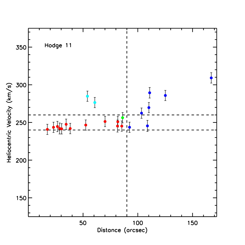
Figure 4: Radial velocities for our spectroscopic targets as a function of distance from the Hodge 11 cluster center. The horizontal lines represent our velocity cut and have a width of $\pm$10 km s^-1. The cluster radius is shown as the vertical line and the color coding of points is discussed in Fig. 3. The errors bars shown represent the random error in determining the radial velocity for each star, where we have added in quadrature the slit centering and cross-correlation errors.

We note that, while this calibration actually combines two metallicity scales (Carretta & Gratton 1997 for the globular clusters and Friel et al. 2002 for the open clusters), C04 find no evidence of age effects on the calibration or any significant deviation from a linear fit to suggest that these two populations are not ultimately on the same [Fe/H] scale (see their Figure 4). Although some of our clusters are likely younger than the 2.5 Gyr age limit established in the calibration of C04, the CaT line strengths for red giants of $\sim$1 Gyr are not expected to deviate strongly from a simple extrapolation of the fitting formula (based on the empirical fitting functions from Cenarro et al. 2002 applied to isochrones published in Girardi et al. 2000), so we use the above calibration for all of our clusters.

3 Analysis

As was mentioned in the previous section, knowledge of the relative brightness of each target star and the cluster HB is imperative to the accurate calculation of $W^{\prime}$ and thus [Fe/H] for each star. To determine $V-V_{HB}$ we utilized the preimages necessary for creating the slit masks used by FORS2. Small aperture photometry was performed on these $V$ and $I$-band images so as to allow us to create cluster CMDs down below the core helium burning red clump stars. For the younger clusters in our sample, $V_{HB}$ was measured as the median magnitude of cluster RC stars. Cluster stars were isolated from the field by selecting stars within the inner half of the apparent cluster radius. We then placed a standard sized box (0.8 mag in $V$ and 0.2 mag in $V-I$) around each cluster RC and used only the stars within this box in our calculation of $V_{HB}$. Regarding clusters with bona fide HBs, i. e. old clusters, we compared our instrumental photometry to published photometry and calculated a rough zeropoint for our data, allowing the conversion of published $V_{HB}$ values onto our instrumental system. Literature sources for the five old clusters are as follows: NGC 1841 $-$ Alcaino et al. (1996); NGC 2019 $-$ Olsen et al. (1998); NGC 2257 and Hodge 11 $-$ Johnson et al. (1999); Reticulum $-$ Walker (1992). Errors in $V_{HB}$ are taken as the standard error of the median for clusters where we measured the RC directly; for the HB in old clusters we adopt 0.1 mag. We note that although we have not calibrated our photometry onto a standard system, the $V-I$ color term for the FORS2 filter system is expected to be small ($<$0.02 mag), thus having little effect on the relative brightnesses of our target stars over the small range of colors covered by the RGB.

3.1 Cluster Membership

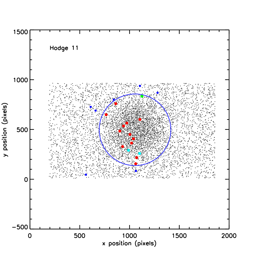
Figure 3: Shown are the $xy$ positions of our target stars (large filled points) on the Hodge 11 field. The adopted cluster radius is marked by the large open circle, and stars outside of this radius are considered non-members. The color coding of symbols in Figs. 3$-$7 is as follows: blue points represent non-members that are outside the cluster radius. Teal and green points are non-members that were cut because of discrepant radial velocities and metallicities, respectively. Finally, red symbols denote cluster members.

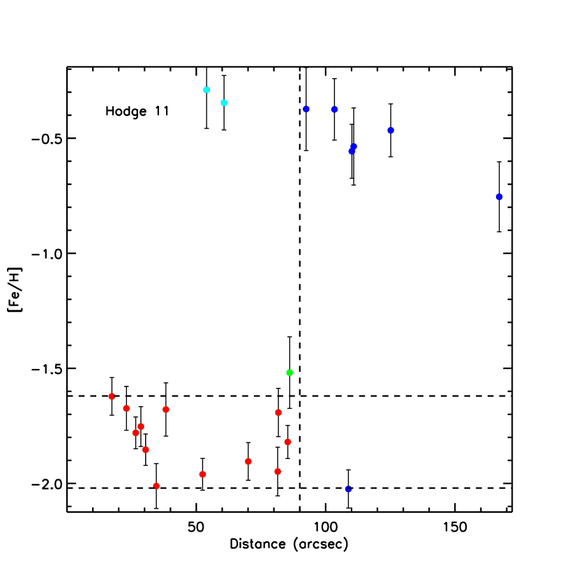
Figure 5: Metallicities are plotted as a function of position for all target stars in Hodge 11. The [Fe/H] cut of $\pm$0.20 dex is denoted by the horizontal lines. For this old, metal-poor cluster, the field ([Fe/H] $\sim$ $-0.5$) is easily distinguished from the cluster (red points). We note that the color coding is the same as for previous figures. The plotted error bars represent the random error in calculating [Fe/H], where we have propogated the error in measuring the equivalent widths through our calculations.

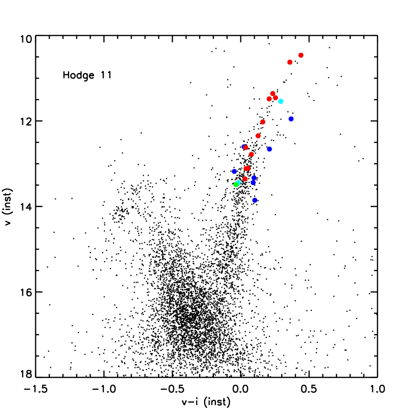
Figure 7: This figure shows the CMD for the entire Hodge 11 field, with target stars marked as described in Fig. 3; cluster members lie along the RGB and AGB.

We use a combination of three criteria to isolate cluster members from field stars. This process is identical for all clusters, so we will illustrate the process using Hodge 11. First, the cluster centers and radii are chosen by eye, based primarily on the photometric catalog. As an example, Fig. 3 shows $xy$ positions for all stars photometered in the Hodge 11 field with large filled points denoting our target stars and the large circle representing the adopted cluster radius; target stars marked in blue (see figure caption for a discussion of the color coding used in Figs. 3$-$7) are considered non-members due to their distance from the cluster center. We note that stars outside of the cluster radius were observed so as to define parameters for the LMC field, which aids in isolating cluster members. Next, radial velocity versus position is plotted in Fig. 4. Stars moving at the velocity of Hodge 11 are easily identified due to their smaller velocity dispersion and lower mean velocity than that of the field stars. Our velocity cut, denoted by the horizontal lines, has been chosen to represent the expected observed velocity dispersion in each cluster. To determine this, we have adopted an intrinsic cluster velocity dispersion of 5 km s^-1 and added this in quadrature with our adopted radial velocity error, 7.5 km s^-1, which results in an expected dispersion of $\sim$ 9 km s^-1. Thus, we have rounded this up and adopted a width of $\pm$ 10 km s^-1 for our radial velocity cut. The cluster radius (vertical line) is marked for reference. Finally, Fig. 5 shows metallicity as a function of position for stars in Hodge 11, with horizontal lines representing the [Fe/H] cut that has been applied to these data. For stars in six of our clusters we have processed both sets of spectra and compared the two [Fe/H] measurements so as to directly determine the metallicity error for each star. Based on these data we find $\sigma_{[Fe/H]}\approx$ 0.15 dex, which we adopt as the random error in [Fe/H] for each star. We have rounded this up to $\pm$ 0.20 dex for use as the metallicity cut shown in Fig. 5. Red filled points denote stars that have made all three cuts and are therefore considered to be cluster members. Since we had no a priori membership information, up to this point we have used a value for $V_{HB}$ which was derived from the entire field, rather than just the cluster. Thus, we have recalculated $W^{\prime}$ (and [Fe/H]) using the appropriate cluster $V_{HB}$ value. In Fig. 6 we present the traditional $\Sigma W$ versus $V-V_{HB}$ plot for cluster members with the dashed line representing the mean metallicity of Hodge 11. The CMD in Fig. 7 shows all stars photometered in the Hodge 11 field; cluster members (red points) lie on the RGB and AGB.

In Table 3, for all stars determined to be members of the observed LMC clusters, we list the following information: stellar identification number, right ascention and declination (as determined from the preimages), heliocentric radial velocity and its associated error, $V-V_{HB}$, and $\Sigma W$ along with the error in measuring $\Sigma W$.

3.2 Cluster Properties

Cluster properties derived from our data are presented in Table 4, with the number of cluster stars given in column 2, the mean heliocentric radial velocities and mean metallicities in columns 3 and 5 and their respective standard error of the mean values in columns 4 and 6. For the clusters SL 4, SL 41, SL 396, Hodge 3, SL 663, and SL 869, we report the first spectroscopically derived metallicity and radial velocity values based on individual stars within these clusters. Additionally, NGC 1718 and NGC 2193 have no previously reported spectroscopic [Fe/H] values, however OSSH derived velocities for these two clusters. Of these eight clusters, NGC 1718 occupies a particularly interesting area of parameter space as it is the most metal poor of our intermediate age clusters, with a metallicity comparable to that of ESO 121 (see discussion in appendix). As mentioned previously, we have not derived values for NGC 1861 since it appears to be younger than 1 Gyr (see appendix).

3.2.1 Metallicities

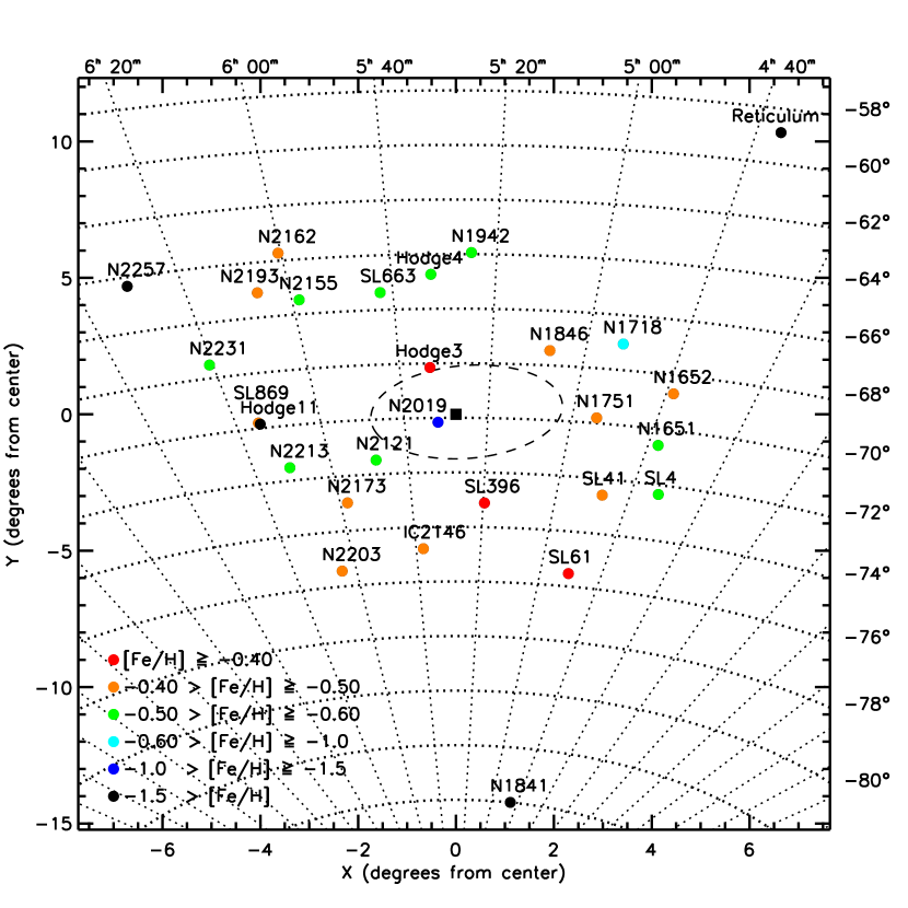
Figure 8: Shown are the positions on the sky and derived metallicities for our target clusters; metallicity bins are given in the lower left corner of the plot. The adopted LMC center is marked with the filled square and the dashed line roughly outlines the bar. See §3.2 for a detailed discussion.

Positions on the sky for each cluster are shown in Fig. 8, along with the metallicity bin into which each cluster falls, represented by the color of the plotting symbol. For two of the higher metallicity bins (orange and green points), the bin size is roughly twice the standard error in [Fe/H], so it is possible that cluster errors could ‘move’ clusters between these and adjacent bins. The adopted center of the LMC ($\alpha=5^{h}27^{m}36^{s}$, $\delta=-69{\arcdeg}52{\arcmin}12{\arcsec}$; van der Marel et al. 2002) is marked by the filled square and the dashed oval represents the 2$\arcdeg$ near-infrared isopleth from van der Marel (2001), which roughly outlines the location of the LMC bar. Conversion from RA and Dec to Cartesian coordinates was performed using a zenithal equidistant projection (e.g. van der Marel & Cioni 2001, their equations 1$-$4); for reference, lines of RA and Dec are marked with dotted lines. In Figs. 9 and 10, we further explore the metallicity/position relationship for LMC clusters by plotting metallicity as a function of deprojected position angle and radial distance (in kpc), respectively. We have corrected for projection effects by adopting 34$\fdg$7 as the inclination and 122$\fdg$5 for the position angle of the line of nodes of the LMC (van der Marel & Cioni 2001). In this rotated coordinate system, a cluster with a position angle of zero lies along the line of nodes, and angles increase counterclockwise; for reference, NGC 2019 has a position angle of $\sim$ 8$\arcdeg$. Radial distances were converted from angular separation to kiloparsecs by assuming an LMC distance of $(m-M)_{0}=18.5$ ($\sim$ 50 kpc); at this distance, one degree is $\sim$ 870 pc. Combined, these three figures illustrate that, similar to what was found by OSSH (and also Geisler et al. 2003), there is no [Fe/H] gradient in terms of either position angle or radial distance for the higher metallicity clusters in our sample. While we cannot make strong comments on the metal poor clusters due to our small sample size, it is well known that a number of metal poor clusters ([Fe/H] $\mathrel{<\kern-10.00002pt\lower 3.87495pt\hbox{$\sim$}}-1.5$) exist in the inner portions of the LMC (e.g. OSSH), suggesting that neither the Population I nor the Population II clusters exhibit a metallicity gradient.

In Fig. 10 we have over plotted both the MW open cluster metallicity gradient from Friel et al. (2002; dashed line) and the M33 gradient from Tiede et al. (2004; solid line). Neither of these disk abundance gradients resembles what we see among the LMC clusters. The question of how to interpret this difference takes us to the work of Zaritsky, Kennicutt, & Huchra (1994). They studied the H II region oxygen abundances in 39 disk galaxies. Their data suggest that disk abundance gradients are ubiquitous in spiral galaxies. However, the presence of a classical bar in the galaxy - one that extends a significant fraction of the disk length - tends to weaken the gradient. This observation seems to find support in the appearance of Fig. 10. In the case of the LMC, the presence of a strong bar component may have diluted the metallicity gradient originally present in the star clusters leading to a cluster population that is well mixed. We note that this result is also consistent with the conclusion of Pagel et al. (1978), who found little evidence for a gradient in oxygen abundance based on a survey of H II regions within 4 kpc of the LMC center. The Pagel result, that $d\log$(O/H)/$d$R $=-0.03\pm 0.02$ dex kpc^-1, parallels our non-detection of a gradient in cluster metallicities.

3.2.2 Kinematics

To characterize the rotation of their clusters, Schommer et al. (1992) fit an equation of the form

$$V(\theta)=\pm V_{m}\{[\tan(\theta-\theta_{0}\sec i^{2}]+1\}^{-0.5}+V_{sys}$$ (4)

to their radial velocity data using a least-squares technique to derive the systemic velocity ($V_{sys}$), amplitude of the rotation velocity ($V_{m}$), and the orientation of the line of nodes ($\theta_{0}$); they adopted an inclination of $27\arcdeg$. Their best fit parameters give a rotation amplitude and dispersion consistent with the LMC clusters having disk-like kinematics, with no indications of the existence of a pressure supported halo. We note that, due to the non-circularity of the LMC, $\theta_{0}$ in Eq. 4 is not the true orientation of the line of nodes (the intersection of the plane of the sky and the plane of the LMC), but rather it marks the line of maximum velocity gradient (van der Marel & Cioni 2001). More recently, van der Marel et al. (2002) used velocities of 1041 carbon stars to study kinematics in the LMC. Similarly, they found that these stars exhibit a disk-like rotation with $V/\sigma$ = 2.9 $\pm$ 0.9, suggesting that these stars reside in a disk that is slightly thicker than the Milky Way thick disk ($V/\sigma$ $\approx$ 3.9).

In Fig. 11, we have plotted Galactocentric radial velocity versus position angle on the sky for our sample, along with velocity data for all clusters listed in Schommer et al. (1992). So as to be consistent with the approach of Schommer et al. (1992), we adopt the Galactocentric velocity corrections given by Feitzinger & Weiss (1979). Additionally, for this figure only, we have adopted their LMC center ($\alpha=5^{h}20^{m}40^{s}$, $\delta=-69{\arcdeg}14{\arcmin}10{\arcsec}$; J2000) for use in calculating the position angles of our clusters. We have used the standard astronomical convention where North has a position angle of zero and angles increase to the East; NGC 1942 has a position angle of $\sim 4\arcdeg$ in this coordinate system. Data from Schommer et al.(1992) are plotted as open circles and our data are plotted as filled stars for the clusters with previously unpublished velocities and filled circles for the remainder of our clusters; overplotted on this figure (dashed line) is the rotation curve solution number 3 from Schommer et al. (1992). For the clusters in common between these two data sets, we find excellent agreement, with a mean offset of 0.15 km s^-1, where our velocities are faster than those of Schommer et al. (1992). Additionally, the derived velocities for the six ‘new’ clusters show that their motions are consistent with the findings of Schommer et al. (1992) in that the LMC cluster system exhibits disk-like kinematics that are very similar to the HI disk, and has no obvious signature of a stellar halo.

4 Comparison with Previous Work

As mentioned in the introduction, OSSH and Suntzeff et al. (1992) have provided the only previous large scale, spectroscopic [Fe/H] calculations for clusters in the LMC. Similar to our work, they utilized the CaT lines as a proxy for measuring Fe abundance directly, but with two important differences: they used the absolute magnitude of their stars, based on the spectral intensity at 8600 Å, as a surface gravity estimator instead of $V-V_{HB}$, and their [Fe/H] calibration is based largely on the Zinn & West (1984) metallicity system, with the addition of two open clusters that have metallicities derived from various spectrophotometric indices (see their table 7). This will introduce two systematic offsets that make it inappropriate to directly compare the OSSH values to our work and other recently measured CaT abundances: first, the use of M₈₆₀₀ creates a dependence on the relative distances of the calibrating clusters and the LMC, and the globular cluster distance scale has been much-revised in the post-Hipparcos era (Reid 1999); and second, it has been shown (e.g., Rutledge et al. 1997b) that the Zinn & West scale is non-linear compared to the more recent Carretta & Gratton (1997) scale based on high-resolution spectra of globular cluster red giants. To put the work of OSSH on the Carretta & Gratton system, Cole et al. (2005) perform a non-linear least-squares fit to calibration clusters in common between their work and that of OSSH. They find that one can estimate the abundance of OSSH clusters on the metallicity system we have used via the following conversion:

$$[Fe/H]\approx-0.212+0.498[Fe/H]_{OSSH}-0.128[Fe/H]^{2}_{OSSH}.$$ (5)

This equation approximates the metallicity that OSSH would have derived from their spectroscopic data and calibration procedure, but with updated metallicities for their calibration clusters; it does not attempt to account for any other differences in the treatment of the data.

In columns 3 and 4 of Table 5 we list [Fe/H] for clusters in OSSH and Suntzeff et al. (1992) in common with our target clusters, where column 3 gives their published values and in column 4 we have converted their numbers onto our metallicity system using Eq. 5; the number of stars used by OSSH in calculating final cluster metallicities is given in parenthesis in column 4 and our derived metallicities are given in column 2 for reference. In Fig. 12 we plot the difference between our metallicities and their converted [Fe/H] values as a function of our metallicities. OSSH give their [Fe/H] errors for an individual star as 0.2 dex, therefore deviations between these data sets as large as $\pm$ 0.2 are not unexpected, suggesting that these results are in relative agreement, with no offset. We note, however, that even with the use of Eq. 5, it is very difficult to directly compare the derived cluster abundances because of the differences in target selection and calibration strategy.

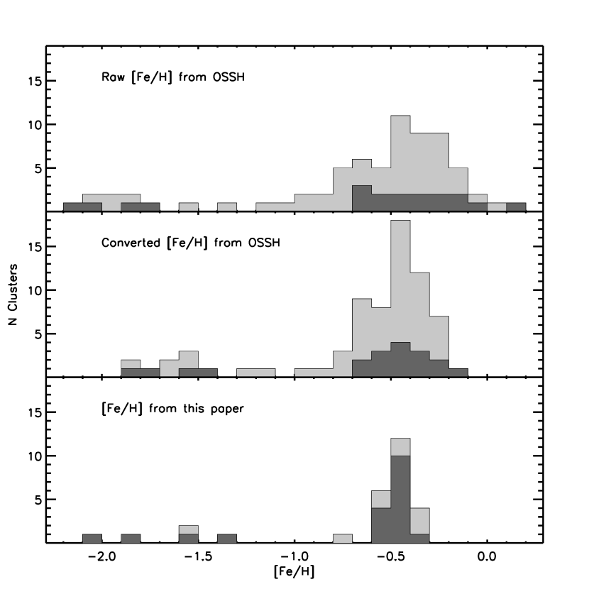
Figure 13: We plot the metallicity distribution of LMC clusters as determined by OSSH and this paper. Published values from OSSH are given in the top panel while the middle panel shows their values converted onto our metallicity scale using Eq. 5; in the bottom panel we have plotted our results. In all three panels, the dark shaded region shows the distribution for the 20 clusters in common between OSSH and this paper, while the light shaded region shows the entire cluster sample from each study. Our results indicate that the LMC’s intermediate age cluster metallicity distribution is actually much tighter than suggested by the results of OSSH.

While a direct comparison of [Fe/H] values is difficult, we can readily compare the metallicity distributions of these two data sets. As such, in Fig. 13, we have plotted the metallicity distribution of OSSH’s raw data (top panel), converted [Fe/H] values (middle panel), and our results (bottom panel). The dark shaded histogram shows only the 20 clusters in common between the three panels, while the lighter histogram plots all clusters in each sample. From this figure it is clear that both the raw and converted OSSH samples show an extended distribution of intermediate metallicity clusters, whereas our cluster sample exhibits a very tight distribution. For the 20 clusters in common, we find a mean [Fe/H] = $-0.47$ with $\sigma=0.06$, while the converted OSSH metallicities give [Fe/H] = $-0.42\pm 0.14$. Our tight metallicity distribution, with a lack of higher metallicity clusters ([Fe/H] $\mathrel{>\kern-10.00002pt\lower 3.87495pt\hbox{$\sim$}}-0.30$), is an important feature of our data for the following reason. Chemical evolution models suggest that metallicity is a rough estimator of age, in that younger stellar populations should be more metal rich than older populations since there has been more time to process material and enrich the ISM. Thus, intermediate age clusters should be more metal poor than younger stellar populations in the LMC. However, some intermediate-age clusters in the sample of OSSH appeared to be more metal-rich than much younger stellar populations in the LMC, which would indicate the presence of a large spread of metallicities at any given age. In Table 6 we give the mean metallicity and spread of our entire sample of intermediate age clusters and all clusters in OSSH with converted metallicities above $-1.0$ dex, along with published results for a sample of younger stellar populations (e.g. B dwarfs, Rolleston, Trundle, & Dufton 2002; Cepheid variables, Luck et al. 1998; young red giants, Smith et al. 2002) and intermediate age RGB field stars in the LMC bar (Cole et al. 2005). This table shows that, as we would expect from chemical enrichment models, the intermediate age clusters are slightly more metal poor than the younger populations in the LMC. Thus, the much tighter metallicity distribution seen in our clusters is in excellent agreement with the expected chemical enrichment pattern in the LMC and alleviates the problem created by the high metallicity tail of intermediate age clusters in the OSSH results. Additionally, Table 6 shows that our intermediate age clusters have a mean metallicity and distribution similar to that of the metal rich component of the bar field studied by Cole et al. (2005). The similarity between these two populations is in good agreement with the models of Bekki et al. (2004), in which the formation of the LMC bar and the restart of cluster formation (end of the ‘age-gap’) are both a result of the same very close encounter with the SMC.

Finally, in Table 5 we have also included [Fe/H] values derived from high resolution spectra for NGC 1841 and NGC 2257 from Hill (2004) and NGC 2019 and Hodge 11 from Johnson et al. (2006). For the two clusters from Johnson et al. (2006), we list [Fe/H] values that are the average of their metallicities determined from Fe I and Fe II lines, and the number of stars observed in each cluster is given. Two clusters, NGC 1841 and NGC 2019, show good agreement between our metallicities, calculated from the CaT lines, and from fitting to high resolution spectra. In contrast, Hodge 11 and NGC 2257 show a roughly 0.3 dex offset between these methods in the sense that our values are more metal rich than the results from high resolution spectra. Similarly, a preliminary result for ESO 121, which is more metal rich than the aforementioned clusters, suggests an offset in the same direction, where the CaT method gives a [Fe/H] value higher than what is measured with high resolution spectra (Cole, private communication). It has been suggested that variations in [Ca/Fe] between calibrating clusters in the MW and target clusters in the LMC may cause a breakdown in the utility of CaT lines as a metallicity indicator. However, abundances based on high resolution spectra show that [Ca/Fe] is typically lower for LMC cluster giants than in MW giants of the same [Fe/H], which is in the opposite direction of what is needed to explain the difference between CaT and high resolution results. We also note that, for low metallicity stars, previous authors have shown that metallicities derived from high-resolution spectra can vary considerably (0.3 dex is not uncommon), depending on which ionization stages, what temperature scale, and what model atmospheres are being used (e.g. Johnson et al. 2006, Kraft & Ivans 2003).

5 Summary

As mentioned in the introduction, determining abundances for populous clusters within the LMC is an important step in understanding the history of this satellite galaxy. Accurate [Fe/H] values help to break the age-metallicity degeneracy that arises when trying to fit theoretical isochrones to cluster CMDs, which will allow the unequivocal determination of cluster ages, thereby providing a clear picture of the LMC’s cluster age-metallicity relation. These clusters also serve to fill a region of the age-metallicity plane that is void of MW clusters; this makes the LMC cluster system an important testbed for a variety of stellar population models. Additionally, in a previous paper (Grocholski & Sarajedini 2002), we have shown that knowledge of a cluster’s age and metallicity is essential to predicting the $K$-band luminosity of the RC for use as a standard candle. In a future work, we will use the metallicities derived herein to determine distances to individual populous LMC clusters, which will allow us to compare the cluster distribution to the LMC geometry calculated from field stars (e.g. van der Marel & Cioni 2001).

In this paper we have presented the results of our spectroscopic study of the near infrared Calcium II Triplet lines in individual RGB stars in 28 populous LMC clusters. Utilizing the multi-object spectrograph, FORS2, on the VLT, we have been able to determine membership and calculate metallicities and radial velocities for, on average, 8 stars per cluster, with small random errors (1.6 km s^-1 in velocity and 0.04 dex in [Fe/H]). The number of cluster members observed, combined with the updated CaT calibration of C04 (they extended the calibration to younger and more metal rich clusters than previous work), has allowed us to improve upon the work of OSSH, which is the only previous large scale spectroscopic study of individual cluster stars within the LMC. The main results of our paper are as follows:

1. We report the first spectroscopically derived metallicities and radial velocities for the following clusters: SL 4, SL 41, SL 396, SL 663, SL 869, and Hodge 3. In addition, NGC 1718 and NGC 2193 have no previously reported spectroscopic [Fe/H] values.

2. NGC 1718 is the only cluster in our sample that falls into the range $-1.3\leq$ [Fe/H] $\leq-0.6$. This metallicity region corresponds to the well known 3$-$13 Gyr ‘age gap,’ within which there is only one cluster, ESO 121. However, unlike ESO 121, the CMD of NGC 1718 suggests an age ($\sim$ 2 Gyr) much younger than the ‘age-gap’; we use archival HST/WFPC2 photometry to investigate this point in the appendix. This age makes NGC 1718 one of the most metal poor intermediate age clusters in the LMC.

3. The intermediate age clusters in our sample show a very tight distribution, with a mean metallicity of $-0.48$ dex ($\sigma$ = 0.09) and no clusters with metallicities approaching solar. While this is in contrast to previous cluster results, it suggests that the formation history of the bar (mean [Fe/H] = $-0.37$, $\sigma=0.15$; Cole et al. 2005) is very similar to that of the clusters. This agrees well with the theoretical work of Bekki et al. (2004), which indicates that a close encounter between the LMC and SMC caused not only the restart of cluster formation in the LMC, but the generation of the central bar as well.

4. Similar to previous work, we find no evidence for the existence of a metallicity gradient in the LMC cluster system. This is in stark contrast to the stellar populations of both the MW and M33, which show that metallicity decreases as galactrocentric distance increases; the LMC’s stellar bar is likely responsible for the well mixed cluster system.

5. We find that our derived cluster velocities, including the six ‘new’ clusters, are in good agreement with the results of Schommer et al. (1992) in that the LMC cluster system exhibits disk-like rotation with no clusters appearing to have halo kinematics.

6. Comparing our results for four clusters to [Fe/H] values recently derived through high-resolution spectra, we find that two of the four clusters are in good agreement, while the other two have [Fe/H] values derived via the CaT method that are $\sim$ 0.3 dex more metal rich than what is found from high-resolution spectra; a similar effect is seen in preliminary results for an additional two LMC clusters. The source of this difference is unclear, however, it is not immediately explained by variations in [Ca/Fe] between the CaT calibration clusters in the MW and the LMC target clusters. Further high resolution studies, especially covering the LMC’s intermediate age clusters, are needed to fully address this issue.

Appendix A Notes on Individual Clusters

A.1 NGC 1718

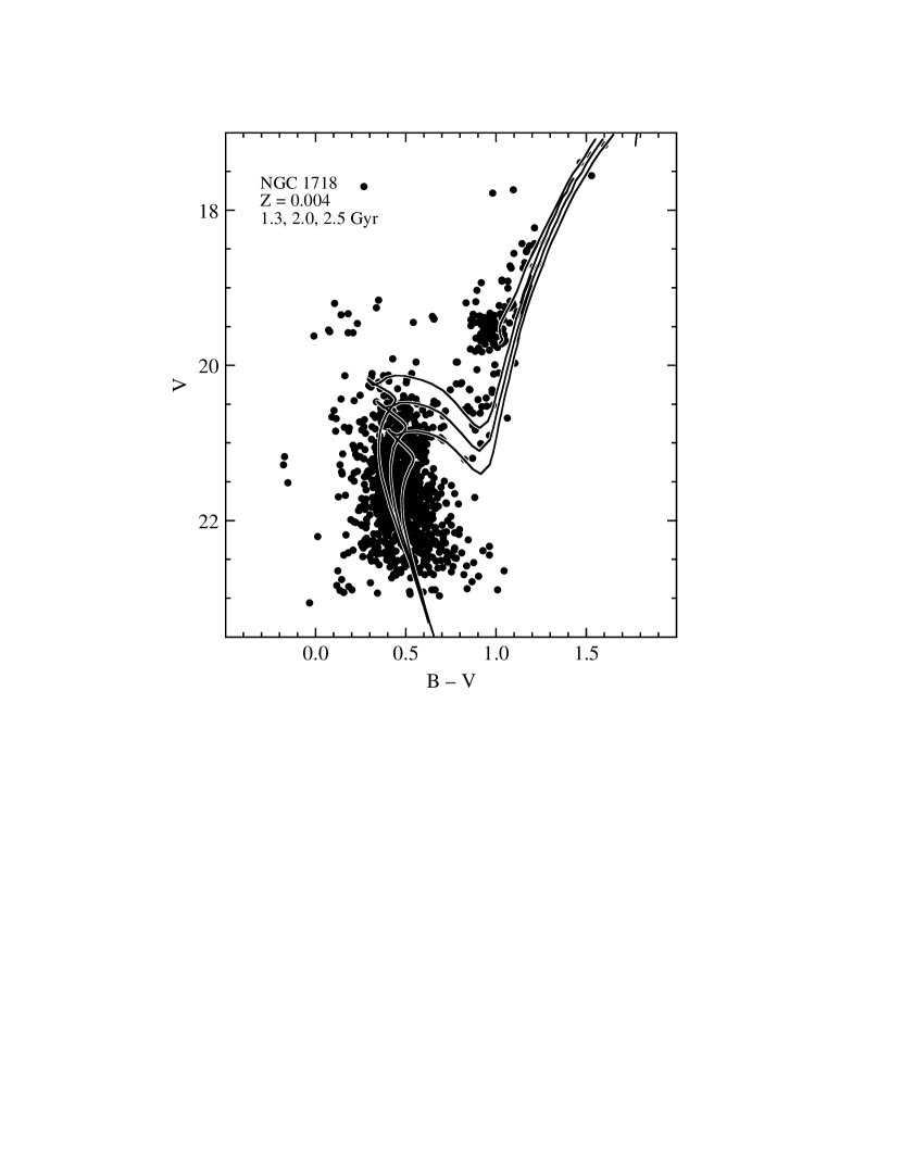
Figure 14: Presented is the cluster CMD for NGC 1718, based on aperture photometry of archival HST/WFPC2 images. We overplot isochrones of 1.3, 2.0, and 2.5 Gyr (top to bottom) from Girardi et al. (2002) that have a metallicity ($\sim$ $-$0.7 dex) similar to the value we have derived for this cluster ($-$0.8 dex). Although this cluster has a metallicity similar to that of ESO 121, the isochrones suggest an age of $\sim$ 2.0 Gyr for this cluster, leaving ESO 121 as the only known LMC cluster with an age between approximately 3 and 13 Gyr.

While only three of the stars observed in NGC 1718 appear to be cluster members, these stars are, on average, 0.3 dex more metal poor than all but one of the other stars observed in this field. As mentioned in §3.2, this causes NGC 1718 to occupy an interesting position in the LMC’s age/metallicity relation; its metallicity is comparable to that of ESO 121, which seems to be the only cluster residing in the LMC having an age between $\sim$ 3 and 13 Gyr (Da Costa 2002). The cluster CMD resulting from our aperture photometry is not well populated around the MSTO, so we have used archival HST/WFPC2 data (GO-5475) to create a cluster CMD reaching below the MSTO. The images were reduced using the procedure outlined by Sarajedini (1998). In summary, all detected stars on the Planetary Camera CCD were photometered in the F450W and F555W filters using a small aperture. These were then corrected to a 0.5 arcsec radius, adjusted for the exposure time, and transformed to the standard system using the equations from Holtzman et al. (1995). In Fig. 14 we present the CMD of NGC 1718 with isochrones from Girardi et al. (2002) overplotted; the isochrones have [Fe/H] $\approx$ -0.7, close to our measured cluster value of -0.8 dex, and ages ranging from 1.3 to 2.5 Gyr. This figure suggests that NGC 1718 has an age of roughly 2.0 Gyr, making it an intermediate age cluster and leaving ESO 121 as still the only cluster known to occupy the LMC’s cluster ‘age gap.’ However, the existence of an intermediate age cluster at this low metallicity is intriguing as it indicates that some pockets of unenriched material must have remained intact even though most of the gas which formed the intermediate age clusters was well mixed.

A.2 NGC 1846

Given the sloped appearance of the RC and the width of the RGB, NGC 1846 is suffering from differential reddening, making it difficult to accurately measure the true location of the cluster RC as well as $V-V_{HB}$ for target stars. To address this problem, we make no adjustments to the instrumental magnitudes, but we measure the median magnitude of the entire differentially reddened RC, effectively measuring the RC at the mean reddening of the cluster. Since the amount of extinction suffered by the RGB stars should be scattered about the mean reddening, this approach will ‘smooth over’ the differential reddening, allowing us to accurately measure the cluster metallicity. We note that this method will increase the scatter in [Fe/H] for cluster members; as such, we have relaxed the metallicity cut in our member selection method to include all stars moving at the radial velocity of the cluster. For reference, if $V-V_{HB}$ for any given star is off by $\pm$ 0.2 mag (we estimate that the differential reddening is 0.4 magnitudes in V), the effect on [Fe/H] for that star is roughly $\pm$ 0.05.

A.3 NGC 1861

This cluster is listed as SWB Type IVB, suggesting an age range of 0.4$-$0.8 Gyr (Bica et al. 1996), which is roughly the age when the RC first forms ($\sim$ 0.5 Gyr; Girardi & Salaris, 2001). Plotting a CMD of stars within the apparent cluster radius reveals what appears to be a fairly young MSTO in addition to no obvious cluster RC or RGB. Therefore, we assume that NGC 1861 is a young cluster and all observed RGB stars are actually part of an older field population.

Figure 2: A sample of spectra from RGB stars in our target clusters covering a range in metallicities. The three CaT lines, along with some nearby Fe I lines, are marked for reference; the change in CaT line strength with [Fe/H] is readily visible. Calculated summed equivalent widths and metallicities for each star are given.

Figure 6: Summed equivalent width versus brightness above the horizontal branch is presented for all stars considered to be members of Hodge 11. The dashed line is an isoabundance line at the mean metallicity of the cluster, [Fe/H] = $-$1.84, and has a slope $\beta$ = 0.73.

Figure 9: We plot the metallicities for our target clusters as a function of deprojected position angle, where we have used the LMC geometry of van der Marel & Cioni (2001) to correct for projection effects. This plot illustrates that there is no apparent relation between position angle and metallicity in the LMC. The error bar shown in the lower lefthand corner of the plot illustrates the average random error in [Fe/H].

Figure 10: Cluster metallicities are plotted as a function of deprojected distance (in kpc) from the center of the LMC; we have assumed a distance of $(m-M)_{0}=18.5$. Overplotted are the metallicity gradients observed in the MW open clusters (dashed line; Friel et al. 2002) and M33 (solid line; Tiede et al. 2004), which help to further illustrate that the LMC’s cluster system lacks the metallicity gradient typically seen in spiral galaxies. This flattened gradient is likely caused by the presence of the central bar (Zaritsky et al. 1994). As with the previous plot, the average random error is illustrated by the error bar on the lower left.

Figure 11: Galactocentric radial velocities as a function of position angle on the sky are plotted for the clusters in our sample (filled symbols) as well as those from Schommer et al. (1992; open circles); the six clusters in our sample with no previous velocity determinations are plotted as filled stars and all others in our sample are filled circles. Rotation curve solution number 3 from Schommer et al. (1992) is overplotted as the dashed line, showing that both data sets are consistent with circular rotation. We note that we have not plotted a representative error bar since our plotting symbols are roughly the same size as the average random velocity error.

Figure 12: Derived metallicities for clusters in common between our study and that of OSSH are compared; we note that [Fe/H] values from OSSH were converted onto the metallicity scale we have used via Eq. 5. This comparison shows that, to within the errors, there is relatively good agreement between our results and those of OSSH (see §4 for more details).

Table 1: LMC Target Cluster Information

Cluster	Alternate	RA	Dec	Diameter	V mag	SWB	Exposure
	name	(J2000)	(J2000)	(arcmin)		Type	Time (s)
SL 4	LW 4	4h32m38s	-72$\arcdeg$20$\arcmin$27$\arcsec$	1.7	14.2	VI	2$\times$300
Reticulum	ESO 118-SC31	4 36 11	-58 51 40	4.7	14.25	VII	2$\times$600
NGC 1651	SL 7, LW 12	4 37 33	-70 35 08	2.7	12.28	V	2$\times$300
NGC 1652	SL 10, LW 14	4 38 23	-68 40 22	1.5	13.13	VI	300
NGC 1841	ESO 4-SC15	4 45 23	-83 59 49	0.9	11.43	VII	500
SL 41	LW 64	4 47 30	-72 35 18	1.4	14.14	V	2$\times$600
SL 61	LW 79	4 50 45	-75 32 00	2.3	13.99	VI	2$\times$300
NGC 1718	SL 65	4 52 25	-67 03 06	1.8	12.25	VI	500
NGC 1751	SL 89	4 54 12	-69 48 23	1.5	11.73	VI	2$\times$300
NGC 1846	SL 243	5 07 35	-67 27 31	3.8	11.31	VI	600
NGC 1861	SL 286	5 10 21	-70 46 38	1.5	13.16	IVB	600
SL 396	LW 187	5 19 36	-73 06 40	1.3	13.56	VI	2$\times$300
NGC 1942	SL 445, LW 203	5 24 43	-63 56 24	1.9	13.46	VI	2$\times$300
NGC 2019	SL 554	5 31 57	-70 09 34	1.5	10.86	VII	600
Hodge 4	SL 556, LW 237	5 32 25	-64 44 12	2.5	13.33	V	500
Hodge 3	SL 569	5 33 20	-68 08 08	1.8	13.42	VI	500
IC 2146	SL 632, LW 258	5 37 46	-74 47 00	3.3	12.41	V	500
SL 663	LW 273	5 42 29	-65 21 48	0.8	13.8	V	600
NGC 2121	SL 725, LW 303	5 48 12	-71 28 52	2.4	12.37	VI	600
NGC 2173	SL 807, LW 348	5 57 58	-72 58 41	2.6	11.88	VI	600
NGC 2155	SL 803, LW 347	5 58 33	-65 28 35	2.4	12.60	VI	600
NGC 2162	SL 814, LW 351	6 00 30	-63 43 19	3.0	12.70	V	2$\times$300
NGC 2203	SL 836, LW 380	6 04 43	-75 26 18	3.2	11.29	VI	500
NGC 2193	SL 839, LW 387	6 06 18	-65 05 57	1.7	13.42	V	600
NGC 2213	SL 857, LW 419	6 10 42	-71 31 44	2.1	12.38	V	2$\times$300
Hodge 11	SL 868, LW 437	6 14 22	-69 50 54	2.7	11.93	VII	600
SL 869	LW 441	6 14 41	-69 48 07	1.6	15.0	VI	600
NGC 2231	SL 884, LW 466	6 20 43	-67 31 07	2.1	13.20	V	500
NGC 2257	SL 895, LW 481	6 30 13	-64 19 29	4.0	12.62	VII	600

Table 2: CaT line and continuum bandpasses

Feature	Line Bandpass (Å)	Blue Continuum (Å)	Red Continuum (Å)
Ca II $\lambda$8498	8490 $-$ 8506	8474 $-$ 8489	8521 $-$ 8531
Ca II $\lambda$8542	8532 $-$ 8552	8521 $-$ 8531	8555 $-$ 8595
Ca II $\lambda$8662	8653 $-$ 8671	8626 $-$ 8650	8695 $-$ 8725

Table 3: Positions and Measured Values for All Cluster Members

ID	RA	Dec	RV	$\sigma_{RV}$	$V-V_{HB}$	$\Sigma W$	$\sigma_{\Sigma W}$
	(J2000)	(J2000)	(km s-1)	(km s-1)	(mag)	(Å)	(Å)
			SL 4
6	4h32m41$\fs$65	-72$\arcdeg$20$\arcmin$59$\farcs$1	237.4	6.7	-0.89	7.65	0.23
7	4 32 40.46	-72 20 50.3	221.6	6.8	-0.64	7.09	0.22
9	4 32 36.78	-72 20 32.2	234.5	6.8	-0.70	6.76	0.31
11	4 32 41.01	-72 20 12.3	221.0	6.9	-1.07	7.59	0.16
12	4 32 39.18	-72 20 00.4	221.3	6.9	-0.03	7.27	0.36
			Reticulum
2	4 36 13.17	-58 52 49.6	250.9	6.8	-1.44	5.37	0.12
3	4 36 14.49	-58 52 40.1	254.3	6.8	-0.81	4.34	0.19
5	4 36 18.63	-58 52 19.6	244.1	7.3	0.78	3.60	0.48
6	4 36 17.19	-58 52 09.6	249.6	7.1	-0.06	3.53	0.33
8	4 36 10.73	-58 51 46.6	245.8	7.1	0.36	3.19	0.46
9	4 36 06.80	-58 51 30.3	251.3	6.9	-1.03	4.33	0.17
11	4 36 07.52	-58 51 11.5	252.8	7.1	-0.53	4.00	0.16
12	4 36 08.07	-58 51 00.6	250.0	7.0	-0.52	4.06	0.24
13	4 36 04.51	-58 50 50.6	237.0	6.7	-0.55	4.47	0.22
14	4 36 01.47	-58 50 33.3	243.1	6.8	0.23	3.88	0.47
15	4 36 09.60	-58 50 23.9	239.9	7.1	-0.33	3.66	0.31
16	4 36 02.14	-58 50 12.6	252.6	7.3	0.07	4.32	0.39
17	4 36 14.10	-58 49 57.0	245.8	6.8	-1.16	4.98	0.12
			NGC 1651
6	4 37 34.49	-70 35 50.2	235.4	6.9	-0.39	6.82	0.25
8	4 37 33.25	-70 35 31.7	235.5	6.7	0.44	6.73	0.79
10	4 37 37.35	-70 35 13.9	223.2	6.8	0.27	6.18	0.46
11	4 37 34.63	-70 35 05.5	233.3	6.8	-1.14	7.88	0.41
12	4 37 34.76	-70 35 02.6	225.4	6.8	-0.87	7.29	0.17
13	4 37 29.94	-70 34 53.8	223.1	6.8	-0.01	6.43	0.35
15	4 37 31.06	-70 34 35.2	237.2	6.8	-1.07	7.74	0.14
16	4 37 31.29	-70 34 25.0	219.2	6.8	-2.26	8.43	0.10
17	4 37 29.58	-70 34 16.0	221.7	7.1	-0.23	6.87	0.26
			NGC 1652
5	4 38 21.50	-68 40 55.4	271.3	6.8	0.02	6.85	0.34
6	4 38 23.75	-68 40 47.1	281.3	6.9	-0.63	7.68	0.26
7	4 38 23.43	-68 40 39.6	276.7	6.8	0.08	6.50	0.52
8	4 38 19.31	-68 40 30.6	272.7	6.8	-0.55	7.34	0.19
9	4 38 19.84	-68 40 20.9	276.3	6.8	-1.59	8.50	0.14
10	4 38 22.03	-68 40 11.1	273.9	6.9	-0.70	7.41	0.22
12	4 38 20.33	-68 39 46.5	277.9	6.9	0.17	6.48	0.48
			NGC 1841
1	4 44 05.58	-84 01 24.0	212.0	6.8	-1.60	3.51	0.16
2	4 44 52.68	-84 01 14.3	205.2	6.9	-1.79	3.88	0.12
4	4 45 27.22	-84 00 53.5	211.8	7.0	-1.18	3.72	0.16
6	4 45 41.54	-84 00 33.7	212.3	6.9	-2.11	4.25	0.10
8	4 44 42.94	-84 00 09.1	212.8	6.9	-0.88	3.41	0.20
9	4 45 19.87	-83 59 59.0	210.4	6.8	-1.49	3.55	0.18
10	4 45 33.89	-83 59 50.4	204.3	6.8	-2.25	4.24	0.12
11	4 45 10.36	-83 59 40.7	204.6	6.8	-1.56	3.80	0.15
12	4 45 15.53	-83 59 29.8	214.3	7.1	-1.27	3.62	0.23
13	4 45 43.84	-83 59 17.7	209.8	6.9	-0.93	3.46	0.22
14	4 45 12.82	-83 59 02.5	207.4	6.9	-0.70	3.30	0.30
15	4 45 28.38	-83 58 48.4	211.3	7.4	-1.52	3.71	0.12
16	4 45 20.51	-83 58 38.4	215.8	6.8	-2.60	4.64	0.10
17	4 46 22.26	-83 58 28.7	212.1	6.9	-1.04	3.18	0.20
19	4 45 55.01	-83 58 00.9	208.9	7.0	-1.29	3.60	0.19
20	4 45 22.59	-83 57 45.5	211.6	6.8	-2.46	4.00	0.11
			SL 41
4	4 47 30.78	-72 35 55.6	223.8	7.1	-0.42	7.29	0.31
5	4 47 29.32	-72 35 42.7	229.0	6.9	-0.13	7.39	0.20
6	4 47 28.06	-72 35 32.0	228.5	6.8	-0.85	7.40	0.15
7	4 47 31.86	-72 35 22.1	230.5	6.7	-1.89	8.20	0.11
8	4 47 32.39	-72 35 14.1	230.5	6.8	-2.33	8.75	0.10
9	4 47 30.92	-72 35 06.0	233.4	7.0	-0.21	7.06	0.22
			SL 61
4	4 50 49.97	-75 32 45.0	224.0	6.8	-0.58	7.58	0.27
8	4 50 44.33	-75 32 07.1	226.1	6.8	-1.07	7.50	0.22
9	4 50 48.31	-75 31 59.2	222.3	6.6	-1.84	8.55	0.18
10	4 50 34.50	-75 31 48.6	215.8	7.0	0.20	7.32	0.62
11	4 50 44.07	-75 31 41.2	227.8	6.8	-1.71	8.32	0.12
12	4 50 50.74	-75 31 31.6	225.5	6.7	-0.15	7.07	0.43
13	4 50 42.63	-75 31 22.9	211.3	7.3	0.14	7.69	0.61
14	4 50 44.32	-75 31 14.1	222.8	6.8	-2.41	9.30	0.11
			NGC 1718
8	4 52 27.20	-67 03 25.7	277.5	6.7	-1.30	7.03	0.25
10	4 52 27.67	-67 03 08.6	275.3	6.7	-1.82	7.34	0.11
13	4 52 20.40	-67 02 38.5	282.6	6.8	-0.59	6.26	0.25
			NGC 1751
5	4 54 19.46	-69 49 18.9	242.8	6.7	-2.21	8.55	0.11
6	4 54 01.54	-69 49 09.0	237.7	6.9	-1.26	7.25	0.21
8	4 54 07.81	-69 48 48.1	249.7	6.7	-2.99	9.48	0.14
10	4 54 08.30	-69 48 20.1	252.1	6.7	-1.63	8.30	0.15
11	4 54 13.67	-69 48 07.2	244.8	6.7	-2.06	8.70	0.11
14	4 54 15.30	-69 47 39.1	245.4	6.8	-1.56	8.09	0.17
			NGC 1846
2	5 07 39.69	-67 28 59.4	233.2	6.7	-1.81	8.37	0.11
4	5 07 32.76	-67 28 31.0	236.2	6.7	-1.39	8.20	0.14
5	5 07 39.03	-67 28 22.3	231.0	6.8	-1.52	8.03	0.12
6	5 07 35.07	-67 28 13.2	240.1	6.7	-0.05	6.92	0.29
8	5 07 33.80	-67 27 56.4	241.1	7.0	-0.12	6.64	0.42
9	5 07 33.87	-67 27 54.6	229.5	7.0	-1.45	7.94	0.11
10	5 07 36.86	-67 27 45.0	234.3	6.8	-2.49	9.28	0.15
11	5 07 39.26	-67 27 35.1	234.8	6.7	-1.98	8.14	0.12
12	5 07 30.12	-67 27 26.5	238.0	6.8	-1.77	8.43	0.10
13	5 07 40.15	-67 27 14.6	235.2	8.4	-0.63	7.08	0.46
14	5 07 35.98	-67 27 06.2	235.3	6.7	-1.51	8.00	0.14
15	5 07 38.81	-67 26 57.7	230.5	6.7	-2.10	8.49	0.11
16	5 07 32.46	-67 26 48.5	232.9	6.7	-1.55	7.70	0.12
17	5 07 33.62	-67 26 40.4	236.8	6.8	-1.98	8.51	0.12
18	5 07 34.04	-67 26 31.8	231.4	6.8	-0.37	6.63	0.22
20	5 07 43.43	-67 26 12.6	235.9	6.8	-0.35	7.16	0.20
21	5 07 33.58	-67 26 02.6	242.4	6.9	-0.33	6.34	0.29
			SL 396
8	5 19 38.32	-73 06 57.8	228.4	6.9	-0.65	7.17	0.18
9	5 19 35.96	-73 06 43.7	224.3	6.7	-1.48	8.14	0.11
10	5 19 38.67	-73 06 37.3	221.7	6.8	-0.91	7.93	0.17
11	5 19 38.97	-73 06 25.7	226.1	6.8	-1.83	8.89	0.13
13	5 19 41.07	-73 06 03.8	225.6	6.8	0.00	6.92	0.35
			NGC 1942
6	5 24 44.67	-63 56 47.2	286.8	6.8	-1.65	8.37	0.13
7	5 24 45.95	-63 56 38.8	298.4	6.8	0.00	6.75	0.24
8	5 24 43.59	-63 56 30.0	286.6	6.8	-1.68	7.63	0.43
9	5 24 46.05	-63 56 20.1	289.6	6.8	-2.43	9.04	0.12
10	5 24 46.56	-63 56 11.8	301.0	6.8	-0.42	7.21	0.20
11	5 24 46.80	-63 56 01.5	299.5	6.6	-0.02	6.72	0.33
12	5 24 41.90	-63 55 51.6	287.8	6.7	-0.83	7.54	0.15
13	5 24 41.84	-63 55 37.9	300.2	7.0	-0.06	6.33	0.28
			NGC 2019
8	5 32 00.40	-70 10 19.1	281.3	6.7	-2.59	6.32	0.09
10	5 32 02.96	-70 10 01.4	287.2	6.8	-2.41	6.83	0.13
11	5 31 59.36	-70 09 51.9	283.6	6.7	-2.60	6.59	0.17
12	5 32 03.01	-70 09 43.9	274.1	6.8	-1.73	5.70	0.14
13	5 31 55.94	-70 09 35.0	276.8	6.8	-1.61	5.39	0.14
			Hodge 4
6	5 32 24.81	-64 44 56.5	317.0	6.8	0.17	6.02	0.29
7	5 32 25.96	-64 44 47.5	301.8	6.8	0.07	6.67	0.30
8	5 32 28.14	-64 44 38.0	309.6	6.8	-0.80	7.75	0.14
9	5 32 24.60	-64 44 30.0	310.9	6.8	-0.82	7.08	0.16
10	5 32 27.95	-64 44 18.4	312.4	6.8	-0.35	7.11	0.21
12	5 32 26.11	-64 43 59.7	315.1	7.0	-0.16	6.37	0.22
13	5 32 25.97	-64 43 47.3	308.7	6.8	-1.73	8.41	0.12
			Hodge 3
5	5 33 14.78	-68 09 50.9	277.0	6.8	-2.16	8.30	0.10
7	5 33 11.87	-68 09 29.3	280.1	6.8	-0.24	7.75	0.33
8	5 33 19.42	-68 09 20.3	279.7	6.8	-0.97	7.68	0.20
10	5 33 22.35	-68 09 10.0	275.8	7.2	-1.54	8.67	0.15
11	5 33 16.19	-68 08 59.8	277.1	6.8	-1.36	8.32	0.15
12	5 33 19.61	-68 08 50.1	277.9	6.8	-2.12	9.25	0.12
13	5 33 20.49	-68 08 35.5	274.4	6.8	-1.60	8.54	0.15
			IC 2146
2	5 37 42.00	-74 48 31.0	224.1	6.7	-0.35	7.04	0.50
3	5 37 37.67	-74 48 20.0	225.4	6.8	-1.57	8.37	0.15
4	5 37 48.70	-74 48 11.0	225.3	6.8	-1.88	8.67	0.15
5	5 37 43.94	-74 48 00.2	224.1	6.8	-2.44	9.24	0.12
7	5 37 38.53	-74 47 40.3	227.6	6.7	-1.55	8.17	0.15
8	5 37 53.30	-74 47 31.6	227.2	6.9	-0.15	7.25	0.49
9	5 37 42.15	-74 47 23.4	223.5	6.8	-1.13	7.60	0.17
10	5 37 43.16	-74 47 13.3	224.4	6.8	-0.65	7.71	0.54
11	5 37 51.92	-74 47 03.4	229.5	6.7	-1.46	8.36	0.13
12	5 37 44.66	-74 46 54.6	227.3	6.8	-0.61	7.52	0.30
13	5 37 45.72	-74 46 46.5	222.6	6.8	-1.31	7.85	0.16
14	5 37 47.30	-74 46 36.7	226.4	6.8	-1.15	7.44	0.21
15	5 37 40.09	-74 46 26.6	231.5	6.8	-0.10	7.34	0.40
16	5 37 40.38	-74 46 15.2	232.3	6.8	-2.49	9.22	0.12
17	5 37 50.48	-74 46 06.6	226.0	6.6	-0.14	6.70	0.56
18	5 38 03.62	-74 45 54.4	225.1	6.8	-2.22	8.80	0.11
19	5 38 03.11	-74 45 45.1	225.7	6.9	-1.05	7.60	0.17
21	5 37 41.58	-74 45 16.8	224.9	6.8	-1.99	8.58	0.11
			SL 663
5	5 42 29.19	-65 22 35.1	299.1	6.7	-1.89	8.57	0.10
8	5 42 30.17	-65 21 59.6	297.3	6.8	-1.17	7.44	0.13
9	5 42 29.59	-65 21 47.3	301.6	6.8	-1.69	8.43	0.15
10	5 42 26.31	-65 21 37.7	303.3	7.0	-0.06	6.28	0.30
11	5 42 29.92	-65 21 29.5	299.8	6.7	-0.07	6.73	0.27
12	5 42 29.07	-65 21 19.4	300.2	6.8	-1.08	7.24	0.14
13	5 42 28.41	-65 21 05.4	299.2	6.8	0.03	6.90	0.36
14	5 42 29.73	-65 20 53.8	311.1	6.8	-0.17	6.59	0.32
			NGC 2121
2	5 48 10.29	-71 30 16.8	228.4	6.7	-2.04	8.60	0.11
7	5 48 07.09	-71 29 24.4	236.5	6.7	-1.30	7.25	0.19
8	5 48 11.85	-71 29 10.9	234.7	6.8	-1.98	8.36	0.10
9	5 48 06.03	-71 29 01.3	233.9	6.8	-1.90	8.51	0.11
10	5 48 22.29	-71 28 46.2	235.4	6.7	-1.45	7.96	0.13
11	5 48 12.54	-71 28 38.0	231.4	6.8	-0.74	7.56	0.18
12	5 48 09.70	-71 28 29.8	239.7	6.8	-1.65	7.83	0.12
14	5 48 15.15	-71 28 12.3	236.2	6.8	-1.70	8.12	0.11
15	5 48 15.71	-71 28 01.6	229.7	6.8	-2.14	8.51	0.12
16	5 47 57.44	-71 27 53.2	227.6	6.9	0.03	6.37	0.23
17	5 48 25.44	-71 27 45.2	227.9	6.8	-1.62	7.81	0.11
20	5 48 13.58	-71 27 11.7	229.0	6.8	-1.87	8.15	0.12
			NGC 2173
6	5 57 54.09	-72 59 11.1	238.5	6.8	-1.37	7.76	0.16
8	5 57 55.77	-72 58 52.4	237.4	6.8	-2.33	8.91	0.12
9	5 57 52.62	-72 58 42.2	235.6	6.8	-2.21	8.67	0.13
10	5 57 57.94	-72 58 29.8	238.6	6.8	-1.87	8.24	0.25
11	5 57 59.18	-72 58 20.8	235.4	6.8	-1.04	7.79	0.19
14	5 57 58.02	-72 57 53.9	239.3	6.8	-2.88	9.41	0.11
			NGC 2155
3	5 58 36.33	-65 29 39.0	310.8	6.8	-1.23	7.94	0.14
5	5 58 37.83	-65 29 13.2	311.7	6.7	-0.83	7.11	0.16
6	5 58 32.85	-65 29 03.4	314.2	6.8	-2.19	8.84	0.12
7	5 58 32.27	-65 28 54.3	308.8	6.8	-0.14	7.04	0.22
9	5 58 28.86	-65 28 38.4	305.9	6.8	-1.72	7.98	0.10
10	5 58 35.94	-65 28 29.3	311.0	6.8	-1.80	8.32	0.12
14	5 58 35.67	-65 27 41.6	301.5	6.7	-0.07	6.21	0.23
			NGC 2162
7	6 00 27.09	-63 43 37.6	323.0	6.8	-1.24	7.49	0.14
8	6 00 28.17	-63 43 28.7	318.1	6.9	-1.20	7.40	0.25
9	6 00 32.04	-63 43 18.0	320.4	6.8	-2.52	8.78	0.13
10	6 00 29.47	-63 43 02.1	335.6	6.8	-1.88	8.39	0.13
11	6 00 27.80	-63 42 51.7	315.9	6.8	0.07	7.52	0.49
			NGC 2203
7	6 04 48.16	-75 26 48.1	244.6	6.7	-1.81	8.18	0.12
8	6 04 40.98	-75 26 39.8	251.2	6.8	-1.78	8.15	0.12
9	6 04 35.08	-75 26 29.2	246.2	6.7	-1.80	8.60	0.14
10	6 04 41.31	-75 26 21.2	249.7	6.8	-1.71	8.39	0.12
11	6 04 33.33	-75 26 13.1	240.1	6.8	-2.07	8.72	0.79
12	6 04 45.42	-75 26 04.0	247.9	6.8	-1.68	8.10	0.12
13	6 04 49.22	-75 25 55.6	247.7	6.8	-2.84	9.55	0.14
14	6 04 43.24	-75 25 45.6	242.2	6.8	-0.74	7.71	0.19
16	6 04 50.33	-75 25 24.2	239.8	6.8	-1.25	7.71	0.14
			NGC 2193
6	6 06 20.10	-65 06 08.0	288.4	6.8	-2.08	8.71	0.10
7	6 06 20.74	-65 05 58.6	287.9	6.7	-1.55	7.78	0.11
8	6 06 18.03	-65 05 48.0	298.8	6.8	-1.63	8.20	0.15
9	6 06 15.56	-65 05 32.3	290.0	6.7	-0.18	6.58	0.25
10	6 06 16.58	-65 05 24.1	291.2	6.8	-0.08	6.97	0.31
			NGC 2213
7	6 10 41.62	-71 32 19.0	238.6	6.7	-1.51	7.84	0.11
8	6 10 45.00	-71 32 00.1	247.1	6.8	-2.18	8.66	0.11
9	6 10 45.68	-71 31 47.1	244.1	6.8	-1.53	8.05	0.13
10	6 10 43.45	-71 31 36.8	240.2	6.8	-0.53	7.08	0.23
11	6 10 39.14	-71 31 33.7	242.7	7.1	-1.95	8.20	0.11
12	6 10 44.25	-71 31 09.4	243.4	6.8	-0.51	6.74	0.20
			Hodge 11
3	6 14 31.61	-69 49 36.5	245.2	6.8	-1.47	4.15	0.12
4	6 14 30.51	-69 49 51.1	251.3	6.9	-0.71	3.36	0.17
7	6 14 21.85	-69 49 57.6	246.6	6.8	-2.01	4.16	0.10
8	6 14 24.80	-69 50 16.6	247.5	7.0	-0.87	3.18	0.23
9	6 14 24.55	-69 50 28.4	243.5	6.8	-2.87	5.57	0.17
10	6 14 21.99	-69 50 33.4	240.8	6.8	-3.03	5.84	0.10
11	6 14 16.88	-69 50 28.0	241.9	7.0	-0.38	3.74	0.27
12	6 14 17.20	-69 50 43.8	241.6	6.8	-2.13	4.54	0.08
13	6 14 17.88	-69 50 54.3	244.6	6.8	-2.03	4.67	0.08
14	6 14 22.57	-69 51 18.8	242.0	7.3	-1.14	4.10	0.18
15	6 14 07.08	-69 50 46.5	250.9	7.2	-0.38	3.71	0.24
18	6 14 08.43	-69 51 22.9	245.2	8.0	-0.14	2.82	0.26
			SL 869
7	6 14 39.08	-69 47 30.6	262.5	6.8	-1.37	7.89	0.14
9	6 14 40.73	-69 47 59.6	256.3	6.8	-1.17	7.93	0.13
11	6 14 44.28	-69 48 46.4	256.4	6.7	-1.27	8.21	0.14
			NGC 2231
3	6 20 41.59	-67 31 45.3	274.5	6.8	-1.09	7.23	0.14
4	6 20 43.41	-67 31 34.7	272.6	6.8	-0.32	6.75	0.22
5	6 20 38.01	-67 31 18.3	274.5	6.7	-2.21	8.73	0.11
6	6 20 45.55	-67 31 06.2	279.4	6.7	-0.53	7.40	0.28
7	6 20 45.24	-67 30 57.3	282.7	6.8	-1.50	7.94	0.12
8	6 20 44.94	-67 30 46.1	278.6	6.7	-1.22	7.39	0.20
9	6 20 48.86	-67 30 36.2	285.1	6.8	-0.51	7.27	0.18
10	6 20 40.00	-67 30 24.2	274.0	6.8	-1.94	8.27	0.12
11	6 20 40.63	-67 30 02.9	277.2	6.7	-0.90	7.39	0.18
			NGC 2257
3	6 30 09.09	-64 20 33.3	302.9	7.0	-0.37	3.94	0.16
4	6 30 14.36	-64 20 23.0	301.1	6.9	-2.30	5.48	0.08
5	6 30 14.94	-64 20 10.0	300.6	6.9	-1.19	4.76	0.12
6	6 30 14.45	-64 20 01.9	303.5	6.9	-0.99	4.73	0.13
7	6 30 07.92	-64 19 53.0	299.9	7.0	-0.41	4.13	0.16
8	6 30 12.16	-64 19 43.5	308.0	6.8	-1.14	4.63	0.18
9	6 30 14.78	-64 19 32.7	296.6	7.0	-1.90	4.88	0.08
10	6 30 10.73	-64 19 24.3	303.4	7.0	-0.21	4.02	0.27
11	6 30 09.22	-64 19 15.4	297.6	6.9	-0.80	4.58	0.16
12	6 30 06.66	-64 19 06.8	297.5	6.9	-0.36	4.10	0.21
13	6 30 14.97	-64 18 58.5	298.9	6.8	-1.85	5.17	0.09
14	6 30 11.03	-64 18 46.6	307.1	7.0	-1.17	4.74	0.14
15	6 30 16.85	-64 18 33.8	302.8	6.9	-0.80	4.08	0.14
17	6 30 27.48	-64 18 07.5	300.7	6.9	-0.82	4.19	0.15
18	6 30 16.26	-64 17 53.8	304.7	7.1	-0.20	4.12	0.22
19	6 30 11.25	-64 17 44.1	299.7	7.3	-0.21	4.21	0.24

Table 4: Derived LMC Cluster Properties

Cluster	n stars	RV	$\sigma_{\overline{RV}}$	[Fe/H]	$\sigma_{\overline{[Fe/H]}}$
Name		(km s-1)	(km s-1)	(dex)	(dex)
SL 4	5	227.1	3.6	-0.51	0.06
Reticulum	13	247.5	1.5	-1.57	0.03
NGC 1651	9	228.2	2.3	-0.53	0.03
NGC 1652	7	275.7	1.3	-0.46	0.04
NGC 1841	16	210.3	0.9	-2.02	0.02
SL 41	6	229.3	1.3	-0.44	0.03
SL 61	8	221.9	2.0	-0.35	0.04
NGC 1718	3	278.4	2.2	-0.80	0.03
NGC 1751	6	245.4	2.1	-0.44	0.05
NGC 1846	17	235.2	0.9	-0.49	0.03
NGC 1861	…	…	…	…	…
SL 396	5	225.2	1.1	-0.39	0.05
NGC 1942	8	293.7	2.3	-0.50	0.04
NGC 2019	5	280.6	2.3	-1.31	0.05
Hodge 4	7	310.8	1.9	-0.55	0.06
Hodge 3	7	277.4	0.8	-0.32	0.05
IC 2146	18	226.3	0.6	-0.41	0.02
SL 663	8	301.4	1.5	-0.54	0.05
NGC 2121	12	232.5	1.2	-0.50	0.03
NGC 2173	6	237.4	0.7	-0.42	0.03
NGC 2155	7	309.1	1.6	-0.50	0.05
NGC 2162	5	322.6	3.5	-0.46	0.07
NGC 2203	9	245.5	1.4	-0.41	0.03
NGC 2193	5	291.2	2.0	-0.49	0.05
NGC 2213	6	242.7	1.2	-0.52	0.04
Hodge 11	12	245.1	1.0	-1.84	0.04
SL 869	3	258.4	2.1	-0.40	0.04
NGC 2231	9	277.6	1.4	-0.52	0.03
NGC 2257	16	301.6	0.8	-1.59	0.02

Table 5: Published LMC Cluster Metallicities

Cluster	[Fe/H]	[Fe/H]	[Fe/H]	[Fe/H]
name	(this work)	CaT	CaT	Hi-Res
SL 4	$-0.51$	…	…	…
Reticulum	$-1.57$	$-1.71$	$-1.44$ (9)	…
NGC 1651	$-0.53$	$-0.37$	$-0.41$ (0.5)	…
NGC 1652	$-0.46$	$-0.45$	$-0.46$ (2)	…
NGC 1841	$-2.02$	$-2.11$	$-1.83$ (8)	$-2.07$
SL 41	$-0.44$	…	…	…
SL 61	$-0.35$	$-0.50$	$-0.49$ (1)	…
NGC 1718	$-0.80$	…	…	…
NGC 1751	$-0.44$	$-0.18$	$-0.31$ (0.5)	…
NGC 1846	$-0.49$	$-0.70$	$-0.62$ (1)	…
SL 396	$-0.39$	…	…	…
NGC 1942	$-0.50$	$+0.16$	$-0.14$ (1)	…
NGC 2019	$-1.31$	$-1.81$	$-1.53$ (1)	$-1.24$ (3)
Hodge 4	$-0.55$	$-0.15$	$-0.29$ (1)	…
Hodge 3	$-0.32$	…	…	…
IC 2146	$-0.41$	$-0.40$	$-0.43$ (2)	…
SL 663	$-0.54$	…	…	…
NGC 2121	$-0.50$	$-0.61$	$-0.56$ (1.5)	…
NGC 2173	$-0.42$	$-0.24$	$-0.34$ (1)	…
NGC 2155	$-0.50$	$-0.55$	$-0.52$ (2.5)	…
NGC 2162	$-0.46$	$-0.23$	$-0.33$ (2)	…
NGC 2203	$-0.41$	$-0.52$	$-0.51$ (2)	…
NGC 2193	$-0.49$	…	…	…
NGC 2213	$-0.52$	$-0.01$	$-0.22$ (1)	…
Hodge 11	$-1.84$	$-2.06$	$-1.78$ (2)	$-2.13$ (2)
SL 869	$-0.40$	…	…	…
NGC 2231	$-0.52$	$-0.67$	$-0.60$ (1.5)	…
NGC 2257	$-1.59$	…	…	$-1.86$

Table 6: Metallicities of Young and Intermediate Age Stellar Populations

Population	Age Estimate	[Fe/H]	$\sigma_{[Fe/H]}$	Reference
	(Myr)
B dwarfs	$<$20	$-0.31$	0.04	Rolleston et al. (2002)
Cepheid variables	10$-$60	$-0.34$	0.15	Luck et al. (1998)
Young RGB stars	200$-$1000	$-0.45$	0.10	Smith et al. (2002)
Intermediate age clusters	1000$-$3000	$-0.48$	0.09	This paper
Intermediate age clusters	1000$-$3000	$-0.48$	0.17	OSSH
Bar RGB stars, metal rich	1000$-$5000	$-0.37$	0.15	Cole et al. (2005)
Bar RGB stars, metal poor	$\mathrel{>\kern-10.00002pt\lower 3.87495pt\hbox{$\sim$}}$5000	$-1.08$	0.47	Cole et al. (2005)

References

- (1) Alcaino, G., Liller, W., Alvarado, F., Kravtsov, V., Ipatov, A., Samus, N., & Smirnov, O. 1996, AJ, 112, 2020
- (2) Armandroff, T.E. & Da Costa, G.S. 1991, AJ, 101, 1329
- (3) Armandroff, T.E. & Zinn, R. 1988, AJ, 96, 92
- (4) Beasley, M.A., Hoyle, F., & Sharples, R.M. 2002, MNRAS, 336, 168
- (5) Bekki, K., Couch, W.J., Beasley, M.A., Forbes, D.A., Chiba, M. & DaCosta, G.S. 2004, ApJ, 610, 93
- (6) Bertelli, G., Nasi, E., Girardi, L., Chiosi, C., Zoccali, M., & Gallart, C 2003, AJ, 125, 770
- (7) Bica, E., Clariá, J.J., Dottori, H., Santos, J.F.C., & Piatti, A.E. 1996, ApJS, 102, 57
- (8) Bica, E.L.D., Schmitt, H.R., Dutra, C.M., & Oliveira, H.L. 1999, AJ, 117, 238
- (9) Brocato, E., Castellani, V., & Piersimoni, A.M. 1994, A&A, 290, 59
- (10) Carretta, E. & Gratton, R.G. 1997, A&A, 121, 95
- (11) Cenarro, A.J., Cardiel, N., Gorgas, J., Peletier, R.F., Vazdekis, A., & Prada, F. 2001, MNRAS, 326, 959
- (12) Cenarro, A.J., Gorgas, J., Cardiel, N., Vazdekis, A., & Peletier, R.F. 2002, MNRAS, 329, 863
- (13) Cole, A.A., Smecker-Hane, T.A., Tolstoy, E., Bosler, T.L., & Gallagher, J.S. 2004, MNRAS, 347, 367 (C04)
- (14) Cole, A.A., Tolstoy, E., Gallagher, J.S., & Smecker-Hane, T.A. 2005, AJ, 129, 1465
- (15) Da Costa, G.S., 1991, in IAU Symp. 148, The Magellanic Clouds, ed. R. Haynes & D. Milne, (Kluwer:Dordrecht), p. 183
- (16) Da Costa, G.S. 2002, in IAU Symp. 207, Extragalactic Star Clusters, ed. D. Geisler, E.K. Grebel, & D. Minitti (San Francisco: ASP), 83
- (17) Da Costa, G.S., & Armandroff, T.E. 1995, AJ, 109, 2533
- (18) Da Costa, G.S., & Hatzidimitriou, D. 1998, AJ, 115, 1934
- (19) Feitzinger, J. & Weiss, G. 1979, A&AS, 37, 575
- (20) Ferraro, F.R., Fusi Pecci, F., Testa, V., Greggio, L., Corsi, C.E., Buonanno, R., Terndrip, D.M., & Zinnecker, H. 1995, MNRAS, 272, 391
- (21) Friel, E.D. & Janes, K.A. 1993, A&A, 267, 75
- (22) Friel, E.D., Janes, K.A., Tavarez, M., Scott, J., Katsanis, R., Lotz, J., Hong, L., & Miller, N. 2002, AJ, 124, 2693
- (23) Geisler, D., Piatti, A.E., Clariá, J.J., & Minitti, D. 1995, AJ, 109, 605
- (24) Geisler, D., Bica, E., Dottori, H., Clariá, J.J., Piatti, A.E., & Santos, J.F.C., Jr. 1997, AJ, 114, 1920
- (25) Geisler, D., Piatti, A.E., Bica, E., Claria, J.C. 2003, MNRAS, 341, 771
- (26) Girardi, L., Bertelli, G., Bressan, A., Chiosi, C., Groenewegen, M.A.T., Marigo, P., Salasnich, B., & Weiss, A. 2002, A&A, 391, 195
- (27) Girardi, L. & Salaris, M. 2001, MNRAS, 323, 109
- (28) Girardi, L., Bressan, A., Bertelli, G., & Chiosi, C. 2000, A&AS, 141, 371
- (29) Grocholski, A.J. & Sarajedini, A. 2002, AJ, 123, 1603
- (30) Hill, V. 2004, in Origin and Evolution of the Elements, ed. A. McWilliam & M. Rauch (Cambridge: Cambridge Univ. Press), 205
- (31) Holtzman, J.A., et al. 1999, AJ, 118, 2262
- (32) Holtzman, J.A., Burrows, C.J., Casertano, S., Hester, J.J., Trauger, J.T., Watson, A.M., & Worthey, G. 1995, PASP, 107, 1065
- (33) Ibata, R.A., Gilmore, G., & Irwin, M.J. 1994, Nature, 370, 194
- (34) Johnson, J.A., Bolte, M., Stetson, P.B., Hesser, J.E., & Somerville, R.S. 1999, ApJ, 527, 199
- (35) Johnson, J.A., Ivans, I.I., & Stetson, P.B. 2006, ApJ, 640, 801
- (36) Jørgensen, U.G., Carlsson, M., & Johnson, H.R. 1992, A&A, 254, 258
- (37) Kim, S., Staveley-Smith, L., Dopita, M.A., Freeman, K.C., Sault, R.J., Kesteven, M.J., & McConnell, D. 1998, ApJ, 503, 674
- (38) Koch, A., Grebel, E.K., Wyse, R.F.G., Kleyna, J.T., Wilkinson, M.I., Harbeck, D.R., Gilmore, G.F., & Evans, N.W. 2006, AJ, 131, 895
- (39) Kraft, R.P. & Ivans, I.I. 2003, PASP, 115, 143
- (40) Leonardi, A.J., & Rose, J.A. 2003, AJ, 126, 1811
- (41) Luck, R.E., Moffett, T.J., Barnes, T.G.III, & Gieren, W.P. 1998, AJ, 115, 605
- (42) Maraston, C. 2005, MNRAS, 362, 799
- (43) Mathieu, R.D., Latham, D.W., Griffin, R.F., & Gunn, J.E. 1986, AJ, 92, 1100
- (44) Mayor, M., et al. 1983, A&AS, 54, 495
- (45) Olsen, K.A.G., Hodge, P.W., Mateo, M., Olszewski, E.W., Schommer, R.A., Suntzeff, N.B., & Walker, A.R. 1998, MNRAS, 300, 665
- (46) Olszewski, E.W., Schommer, R.A., Suntzeff, N.B., & Harris, H.C. 1991, AJ, 101, 515 (OSSH)
- (47) Osterbrock, D.E. & Martel, A. 1992, PASP, 104, 76
- (48) Pagel, B.E.J., Edmunds, M.G., Fosbury, R.A.E, & Webster, B.L. 1978, MNRAS, 184, 569
- (49) Persson, S.E., Aaronson, M., Cohen, J.G., Frogel, J.A., & Matthews, K. 1983, ApJ, 266, 105
- (50) Rolleston, W.R.J., Trundle, C., & Dufton, P.L. 2002, A&A, 396, 53
- (51) Rutledge, G.A., Hesser, J.E., Stetston, P.B., Mateo, M., Simard, L., Bolte, M., Friel, E.D., & Copin, Y. 1997a, PASP, 109, 883
- (52) Rutledge, G.A., Hesser, J.E., & Stetson, P.B. 1997b PASP, 109, 907
- (53) Sarajedini, A. 1998, AJ, 116, 738
- (54) Schommer, R.A., Olszewski, E.W., Suntzeff, N.B., & Harris, H.C. 1992, AJ, 103, 447
- (55) Searle, L. & Zinn, R. 1978, ApJ, 225, 357
- (56) Smecker-Hane, T. A., Cole, A. A., Gallagher, J. S., & Stetson, P. B. 2002, ApJ, 566, 239
- (57) Smith, V.V., et al. 2002, AJ, 124, 3241
- (58) Stetson, P.B. 1987, PASP, 99, 191
- (59) Suntzeff, N.B., Schommer, R.A., Olszewski, E.W., & Walker, A.R. 1992, AJ, 103, 1166
- (60) Staveley-Smith, L., Kim, S., Calabretta, M.R., Haynes, R.F., & Kesteven, M.J. 2003, MNRAS, 339, 87
- (61) Tiede, G.P., Sarajedini, A., & Barker, M.K. 2004, AJ, 128, 224
- (62) Tolstoy, E., Irwin, M.J., Cole, A.A., Pasquini, L., Gilmozzi, R., & Gallagher, J.S. 2001, MNRAS, 327, 918
- (63) Tonry, J., & Davis, M. 1979, AJ, 84, 1511
- (64) van der Marel, R.P. 2001, AJ, 122, 1827
- (65) van der Marel, R.P. & Cioni, M.-R. L. 2001, AJ, 122, 1807
- (66) van der Marel, R.P., Alves, D.R., Hardy, E., & Suntzeff, N.B. 2002, AJ, 124, 2639
- (67) Walker, A.R. 1992, AJ, 103, 1166
- (68) Zaritsky, D., Kennicutt, R. C., Jr., & Huchra, J. P. 1994, ApJ, 420, 87
- (69) Zentner, A.R., & Bullock, J.S. 2003, ApJ, 598, 49
- (70) Zinn, R. & West, M.J. 1985, ApJS, 55, 45