Strong lensing statistics in large, $z\mathrel{\hbox{\hbox to0.0pt{\hbox{\lower 4.0pt\hbox{$\sim$}}\hss}\hbox{$<$}}}0.2$ surveys: bias in the lens galaxy population

Abstract

Large current and future surveys, like the Two degree Field survey (2dF), the Sloan Digital Sky Survey (SDSS) and the proposed Kilo-Degree Survey (KIDS) are likely to provide us with many new strong gravitational lenses. Taking cosmological parameters as known, we calculate the expected lensing statistics of the galaxy population in large, low-redshift surveys. Galaxies are modeled using realistic, multiple components: a dark matter halo, a bulge component and disc. We use semi-analytic models of galaxies coupled with dark matter haloes in the Millennium Run to model the lens galaxy population. Replicating the selection criteria of the 2dF, we create a mock galaxy catalogue. We predict that a fraction of $1.4\pm 0.18\times 10^{-3}$ of radio sources will be lensed by galaxies within a survey like the 2dF below $z<0.2$. We find that proper inclusion of the baryonic component is crucial for calculating lensing statistics – pure dark matter haloes produce lensing cross sections several orders of magnitude lower. With a simulated sample of lensed radio sources, the predicted lensing galaxy population consists mainly of ellipticals ($\sim 80\%$) with an average lens velocity dispersion of $164\pm 3\,\mathrm{km\,s^{-1}}$, producing typical image separations of $\sim 3\arcsec$. The lens galaxy population lies on the fundamental plane but its velocity dispersion distribution is shifted to higher values compared to all early-type galaxies. We show that magnification bias affects lens statistics very strongly and increases the 4:2 image ratio drastically. Taking this effect into account, we predict that the ratio of 4:2 image systems is $30\pm 5\%$, consistent with the observed ratio found in the Cosmic Lens All-Sky Survey (CLASS). We also find that the population of 4-image lens galaxies differs markedly from the population of lens galaxies in 2-image systems. We find that while most lenses tend to be ellipticals, galaxies that produce 4 image systems preferentially tend to be lower velocity dispersion systems with more pronounced disc components. Our key result is the explicit demonstration that the population of lens galaxies differs markedly from the galaxy population as a whole: lens galaxies have a higher average luminosity and, for a given luminosity, they reside in more massive haloes than the overall sample of ellipticals. This bias restricts our ability to infer galaxy evolution parameters from a sample of lensing galaxies.

1 Introduction

Individual lens modeling has already provided many interesting constraints on the mass profile of clusters and galaxies (e.g. Schechter et al., 1997; Cohn et al., 2001; Rusin & Ma, 2001; Wyithe et al., 2002; Kneib et al., 2003; Treu & Koopmans, 2003; Broadhurst et al., 2005). In the case of galaxy lenses, the measured time-delays between the multiple images has been used to determine bounds on the value of the cosmological constant (e.g. Rhee, 1991; Koopmans & Treu, 2003) and the Hubble constant (Kundic et al., 1997b; Schechter et al., 1997; Ferreras et al., 2005). The cosmological density parameters, $\Omega_{\Lambda}$ and $\Omega_{m}$ have also been estimated using a sample of gravitational lens systems (Helbig et al., 1999; Meneghetti et al., 2005; Dalal et al., 2005; Chae, 2003). However, despite great efforts, modeling of individual gravitational lens systems has not yet provided constraints on any of the cosmological parameters comparable to those from other techniques like the studies of the Cosmic Microwave Background Radiation. The primary reason for this is that there are many degeneracies in the lens models which are still poorly understood. Since the details of the mass models have considerable effect on the derived cosmological parameters, lens model degeneracies pose a fundamental limitation in exploiting lensing (Möller & Blain, 1998; Wucknitz, 2002; Zhao & Qin, 2003).

A second possibility to constrain cosmology from lensing is to use lens statistics. With a large sample of observed lenses, the average mass properties of the galaxy population become more important and hence the results are largely independent of individual deviations in the lens mass distributions. This then also enables constraints on the mass properties of the galaxy population as a whole to be obtained.

Even though cosmology crucially affects lensing statistics (e.g. Turner et al., 1984; Fukugita et al., 1992; Kochanek, 1993; Chae, 2003), several effects complicate the connection. The source properties, like source redshift distribution and luminosity function, together with magnification bias, all affect lensing statistics strongly. There is furthermore, degeneracy between lens models, statistical source properties, magnification bias and cosmological parameters. Previous constraints on cosmological parameters from strong lensing are thus not directly comparable in precision to other techniques like constraints from experiments such as the WMAP space mission (Spergel et al., 2006). It is perhaps more fruitful to take the cosmological parameters as “known” quantities and use lensing statistics instead to constrain the properties of the lensing galaxy population. This is the approach that we explore in this work.

The statistics of strong lensing by galaxies has been studied by several authors in the past (Turner et al., 1984; Fukugita et al., 1992; Kochanek, 1993; Möller & Blain, 2001; Chae, 2003). Most of these studies calculate a lensing cross section analytically using a simple lens model along with known mass and luminosity functions. Others are concerned with the effect of specific details of the mass models on the lens statistics or properties of the source population (Huterer et al., 2005). On larger scales, the arc-statistics of galaxy clusters has been used to constrain cosmological parameters (Bartelmann et al., 1998; Meneghetti et al., 2005; Dalal et al., 2005). Perhaps due to the limited sample of galaxy lens systems known, the interest in statistical lensing on galaxy scales has so far concentrated mainly on predicting the number of strongly imaged systems using simple lens models. However, the number of known lens systems is increasing steadily and in the near future many large surveys are likely to detect a significantly increased number of strong lens systems. Such a large number of lens systems could potentially constrain masses of galaxies and provide important constraints on the mass evolution of galaxies between $z\sim 0.1$ and $z\sim 1$. Thus, statistical lensing is potentially a very important tool for galaxy evolution studies.

Detailed statistical lens studies have so far been hampered by the lack of a clearly defined lens sample. Most known lens systems have been discovered serendipitously and comprehensive surveys like the Cosmic Lens All-Sky Survey (CLASS) are rare. Simple estimates of the lensing probability suggest the fraction of sources at $z\sim 1$ being lensed into multiple images is between $10^{-4}$ and $10^{-2}$. The largest current survey, the Sloan Digital Sky Survey (SDSS), contains about 500,000 foreground galaxies and about 100 million background galaxies at higher redshifts, and should thus contain at least several thousand lensed galaxies.

In this paper, we use semi-analytic models of galaxy formation (Kauffmann et al., 1993; Somerville & Primack, 1999; Kauffmann et al., 2004; Bower et al., 2006; Croton et al., 2006) to predict the statistical properties of a large sample of strong lenses that would be detected by surveys in the radio, optical and infrared wavebands. We concentrate here on radio sources that are lensed by low redshift galaxy lenses with $z_{\mathrm{lens}}<0.2$, as environmental effects are smaller for such a population. Two large surveys with similar redshift limits have been carried out to date, the Sloan Digital Sky Survey (SDSS Adelman-McCarthy et al., 2006) and the Two Degree Field Survey (2dF Colless et al., 2001). Even though we use the 2dF as a template survey for this work, our results are equally valid for the SDSS. In particular, we predict the expected lensing properties of galaxies in these surveys. This is done by calculating the lensing properties of a mock survey catalogue obtained from the semi-analytic models assuming a composite mass model consisting of dark matter halo (DM), bulge and disc for lens galaxies. The lensing cross section, image geometries and magnifications are calculated for each galaxy individually using numerical routines. From these we then create a sample of lens systems, which we then analyse further.

We describe the use of semi-analytic methods to create the lens mass models and outline the method to calculate lensing probabilities in detail in § 2. In § 3 we show the predicted statistical lensing properties of galaxies in low redshift surveys and the dependence on galaxy properties. In § 4 we apply specific selection criteria and predict the properties of a radio selected sample of lenses with $z_{\mathrm{l}}<0.2$. Our results are presented in § 5, including the predictions for the lensing rate. In § 6 we summarize our key results and discuss their implications. Throughout this paper we use a standard $\Lambda$CDM cosmology with $\Omega_{\Lambda}=0.75$, $\Omega_{\mathrm{m}}=0.25$ and $H_{0}=73\,\mathrm{km\,s^{-1}\,Mpc^{-1}}$.

2 The mock lens catalogue

We use the Millennium Run numerical simulation (Springel et al., 2005) together with semi-analytic modelling of galaxy formation to predict the properties of the dark and luminous matter in galaxies and thereby derive the expected lensing statistics in large surveys at $z\mathrel{\hbox{\hbox to0.0pt{\hbox{\lower 4.0pt\hbox{$\sim$}}\hss}\hbox{$<$}}}0.2$. In the procedure used for semi-analytic modeling a catalogue of halo and substructure is generated at closely spaced redshift intervals, and for each individual $z=0$ DM halo a corresponding merger tree is identified. The prescription described in Croton et al. (2006) is used to follow stellar masses, luminosities and morphologies of galaxies that assemble in these DM haloes. From these, we create a mock low redshift galaxy catalogue that is similar to the 2dF North field by applying the same selection cuts in magnitude and redshift. We describe the creation of this mock 2dF galaxy catalogue below. The parent DM haloes are taken from the Millennium Run. Selection of simulated haloes is done by defining a backward lightcone from $z=0$. Even though we use the creation of a backward lightcone, we note that for most of the work presented here, the creation of a full light cone is not strictly necessary, as we treat galaxies as isolated in our lensing analysis. In this treatment, we are ignoring the immediate environments of haloes while calculating lensing cross sections and image geometries. It is well documented that the presence of mass concentrations in the vicinity of lenses impacts the image separation distribution(Möller & Blain, 2001) and we address this interplay in future work.

2.1 Making mock observations

We construct mock observations of our artificial Universe in the Millennium simulation by positioning a virtual observer in the simulation at zero redshift and finding those galaxies which lie on the observer’s backward lightcone. The main limitation in producing a mock observation of a simulation is the finite box size, which in this case is $500\,h^{-1}\rm{Mpc}$ on a side. The periodic nature of the simulation allows us to fill the space with any number of boxes we require but we still have to deal with periodic replications that would appear if we were to look through the simulation volume along one of its preferred axes. We can avoid this kaleidoscopic effect through slanting the observed cone by a certain angle. After having determined the survey geometry, observer position and line-of-sight we fill the four-dimensional Euclidean space-time with a grid of simulation boxes. In the three spatial coordinates we make use of the periodicity of the simulation whereas the time coordinate is given by the 64 snapshot times corresponding to their respective output redshifts. In practice, only those cells in the space-time grid are populated with galaxies which actually intersect the backward lightcone in the observed field-of-view. After coarsely filling the volume around the observed lightcone with simulation boxes in this way one can simply “chisel off” the protruding volume.

We note that by using comoving coordinates and assuming a flat Universe we have the luxury of cutting the lightcone from our simulated volume simply like we would in Euclidean geometry. In general this is a non-trivial endeavour that requires taking into account the curvature of the Universe as well as its expansion with time.

2.2 Lensing probabilities for an SIS model

Before calculating the lensing cross section for realistic mass models of lensing galaxies we first discuss the singular isothermal sphere (SIS) model that has in the past most commonly been used for statistical lensing calculations (e.g. Turner et al., 1984; Fukugita et al., 1992). Despite its simplicity the SIS model has been surprisingly successful in describing the overall statistical properties of galaxy-scale lenses. As shown by Koopmans & Treu (2002, 2003), the stellar component of lens galaxies has a density profile that is much steeper at than the dark matter at small radii so that the total mass profile (including dark matter) follows an isothermal profile on scales probed by galaxy strong lensing more closely, thereby explaining the modelling success of the SIS. For most groups and cluster lenses, however, the SIS model is an inadequate description of the total mass distribution. On cluster scales the baryonic component becomes less important and the lensing profile is more accurately modeled using a Navarro, Frenk & White profile (NFW Navarro et al., 1997) well beyond the arc radius (Kneib et al., 2003). For lower redshift lenses, the Einstein radius is small compared to the galaxy size and the relative DM mass content within the Einstein radius is smaller. Thus, for all galaxies (excluding the most massive groups and clusters), the baryonic galaxy component of the mass profile dominates the lensing cross section at low redshifts.

The lensing cross sections of a SIS model for elliptical galaxies can be calculated directly from the observed Faber-Jackson relation. The lensing cross section of an SIS is given by:

$$\tau_{\rm SIS}=64\pi\left(\frac{\sigma}{c}\right)^{4}\left(\frac{D_{\mathrm{LS}}}{D_{\mathrm{OS}}}\right)^{2},$$ (1)

the total lensing probability can be calculated using the luminosity function $N(L)$ of galaxies:

$$\tau\propto\int_{0}^{\infty}\sigma(L)^{4}N(L)\,dL,$$ (2)

where

$$\sigma(L)=\sigma_{*}\left(\frac{L}{L_{*}}\right)^{\beta}$$ (3)

is the Faber-Jackson relation. Using the 2dF luminosity function Norberg et al. (2002) fit, we have:

$$\tau=\int_{z=0}^{\infty}\,\tau_{*}\,\left(\frac{D_{\mathrm{LS}}}{D_{\mathrm{OS}}}\right)^{2}\,\phi_{*}\left[\frac{\sigma}{\sigma_{*}}\right]^{4}\,\left(\frac{L}{L_{*}}\right)^{\alpha}\,\exp{(-\frac{L}{L_{*}})}\frac{dV_{\mathrm{co}}}{dz}\,dz$$ (4)

where $\phi_{*}=1.64\times 10^{-2}\,\mathrm{Mpc}^{-3}$, $\alpha=-1.21$, $L_{*}=1.82\times 10^{10}L_{\odot}$ and $\tau_{*}=(\sigma_{*}/\mathrm{km\,s^{-1}})^{4}\times 1.055\times 10^{-9}\,\mathrm{arcsec}^{2}$ is the characteristic lensing cross section of an $L_{*}$ galaxy for equal distances $D_{\mathrm{LS}}$ and $D_{\mathrm{OS}}$. The comoving volume of a shell of thickness $dz$ is given by $dV_{\mathrm{co}}/dz\times dz$.

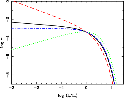
Figure 1: The lensing cross section for SIS lenses with sources at $z=2$ for different slopes of the luminosity function and power-law indices relating luminosity and velocity dispersion. The solid line shows the results for $\alpha=-1.21$ and $\beta=0.25$, corresponding to the 2dF results. The dashed, red line is for $\alpha=-2$ and $\beta=0.25$ and the dotted green and dot-dashed blue lines are for $\alpha=-1.21$ and $\beta=0.31$ and $\beta=0.5$ respectively. The functional form of the luminosity function is given in equation 3.

We show the $\tau-L$ relation for various choices of $\alpha$ and $\beta$ in Fig. 1. For a slope of the Faber-Jackson relation of $\beta<0.3$ the lensing cross section $\tau(L)$ is a monotonically decreasing function with L. In the case of an SIS lens, the largest contribution to the total lensing cross section is expected from the galaxy population around $L_{*}$. Using the Faber-Jackson relation determined from early-type galaxies in the SDSS (Bernardi et al., 2003a), with $\beta=1/4$ and $\sigma_{*}=\sigma(L_{*})=166.44\,\mathrm{km\,s^{-1}}$, we obtain a total lensing cross section of:

$$\tau_{\mathrm{tot}}=\int_{L=0}^{\infty}\tau(L)\,dL=8.36\times 10^{-3},$$ (5)

for sources at $z_{\rm sources}=2$. This is our first and simplest estimate of the expected lensing rate. At this juncture, we have neglected the fact that galaxies contain DM and baryons which are, in general, not expected to be distributed isothermally. The measured velocity dispersion may be biased with respect to the velocity dispersion inferred for the dark matter. In addition, we have also neglected magnification bias and the source luminosity and redshift distributions.

2.3 Towards realistic lens models: dark matter and baryons

More sophisticated models than the SIS have been used by e.g. Oguri et al. (2005) who predicted the lensing statistics in the SDSS using a spherical Hernquist model for the baryons and an NFW dark matter mass profile. Spherical models do predict the overall lensing cross section with adequate accuracy (Fukugita et al., 1992). They cannot, however, predict any detailed properties, like the average magnification and the statistics of image geometries. For instance, the number of four image systems predicted by spherical lens models is zero. We use the ray-tracing code gLens (Möller & Blain, 1998) to calculate the lensing properties of multi-component lens systems efficiently. In order to calculate expected lensing properties of galaxies in large surveys, we need to relate the observed properties, like luminosity and size to a mass model. Since lensing is sensitive to the total mass, we need to include the contributions both of the baryonic and of the dark matter. Our galaxy model therefore consists of a baryonic component, modeled as a bulge of mass $M_{\mathrm{b}}$ plus a disc of mass $M_{\mathrm{d}}$ that reside in a DM halo of virial mass $M_{\mathrm{vir}}$.

In this paper, we consider only the lensing statistics of isolated lenses. In reality, most lens galaxies are expected to reside in dense environments, in groups or clusters (Kundic et al., 1997a; Möller et al., 2002; Keeton & Zabludoff, 2004; Oguri et al., 2005). However, the lens galaxies we consider here are all at relatively low redshifts, where the effect of environment is expected to be less strong. At redshifts $z\leq 0.2$ the expected Einstein radius is small compared with the distance to nearest neighbours (this is true even for lens galaxies in groups and clusters). We note that by construction our catalogue also includes the total lensing cross section by groups and clusters: the haloes of these objects, together with their central galaxy, are included in our catalogue as single, isolated galaxies. In this sense, our calculations are complete, except that they do not take into account the effects of satellite galaxies and external shear deriving from neigbouring mass concentrations and halo substructure within these DM haloes.

2.3.1 Modeling the dark matter halo

N-body simulations of structure formation in a cold dark matter dominated Universe find that the best-fit density profile for dark matter haloes follows a universal functional form over a broad range of scales (Navarro et al., 1997). The mass distribution for a spherical NFW halo is given by,

$$\rho(r)=\frac{\delta_{c}\rho_{c}(z)}{\frac{r}{r_{s}}\left(1+\frac{r}{r_{s}}\right)^{2}},$$ (6)

where $r_{s}=R_{\mathrm{vir}}/c$ is the scale length, $\rho_{c}(z)$ is the critical density for closure at the galaxy redshift and

$$\delta_{c}=\frac{200/3\,c^{3}}{\log{(1+c)}-c/(1+c)}.$$ (7)

The concentration parameter $c$ is ultimately a unique property for each halo in simulations, however correlations (with some scatter) between the concentration parameter and the mass or virial velocity of the halo have been found (Navarro et al., 1997; Bullock et al., 2001; Eke et al., 2001). A closer investigation of the strong lensing by NFW haloes reveals that the lensing cross section depends crucially on the concentration parameter. For the same halo mass, a halo with $c=20$ has a lensing cross section that is $\sim$10 times higher than a halo with $c=10$, and $\sim 100$ times higher than a halo with $c=5$. This implies that the scatter in these correlations between halo mass and central concentration parameter is very important for lensing – most of the lensing cross section contribution derives from massive, high concentration ‘outliers’. Due to this effect, the lensing statistics of a galaxy population can only be correctly predicted if the full scatter in the distribution function of the concentration parameter is taken into account. In this work, we calculate the concentration parameter explicitly for each halo. For this, we use the equation (Navarro et al., 1997),

$$\frac{V_{\mathrm{max}}}{V_{\mathrm{vir}}}=\sqrt{0.216\frac{c}{A_{\mathrm{c}}}},$$ (8)

where

$$A_{\mathrm{c}}=\ln{(1+c)}-\frac{c}{1+c}.$$ (9)

For each halo in the simulation, the parameters $V_{\mathrm{max}}$ and $V_{\mathrm{vir}}$ are known and we use the eqns. (8) and (9) to calculate the concentration parameter for each halo. This procedure ensures that the distribution of concentration parameters automatically has the correct scatter.

2.3.2 Modeling the baryonic components

The baryonic mass is distributed into a bulge and a disc component. The relation between the mass of a DM halo and the luminosity of the baryonic component can be studied using semi-analytic models of galaxy formation. The semi-analytic prescription of Croton et al. (2006) gives a bulge luminosity, a disc luminosity and a disc size.

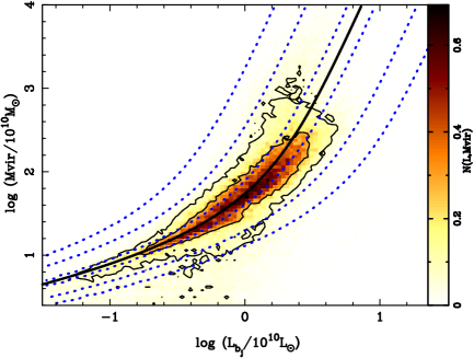
Figure 2: The relation between the halo virial mass $M_{\mathrm{vir}}$ and galaxy luminosity in the $B_{j}$-band. The shading shows the number of galaxies in the mock 2dF catalogue created from the Millennium Run (Springel et al., 2005) combined with the semi-analytic model of Croton et al. (2006). The black line shows the relation in the $B_{j}$-band obtained by Vale & Ostriker (2004). The dotted blue lines show the 68, 90 and 99 percent levels of the scatter around the mass-luminosity relation as obtained by Cooray & Cen (2005).

We show the mass-luminosity relation for our mock catalogue in Fig. 2. For comparison, we overplot the relation

$$L_{Bj}/10^{10}L_{\odot}=0.3\frac{(M_{\mathrm{vir}}/10^{11}M_{\odot})^{4}}{\left(0.57+(M_{\mathrm{vir}}/10^{11}M_{\odot})^{0.79}\right)^{1/0.23}}.$$ (10)

derived by Vale & Ostriker (2004) as the solid line, including the scatter (dotted, blue line). Note that there are galaxies in the catalogue that consistently fall above and to the left of the analytic relation (given in eqn. 10) for high virial masses, which correspond to central galaxies in the more massive haloes of clusters or groups.

2.3.3 The Bulge component

The size and velocity dispersion of the bulge component is not determined in the semi-analytic modelling. However, the distribution of bulge sizes is known observationally (de Jong et al., 2004). There are no models that relate the bulge size to properties of the DM halo. The fundamental plane relation suggests that DM haloes and the bulge properties are related: virialised haloes with constant M/L will naturally lie on the fundamental plane, but so far no theoretical model has been developed that naturally explains both the existence and the slope of the fundamental plane. In the absence of such a model, we rely on the observed relations between luminosities and sizes of elliptical galaxies and apply these to the population of bulges as a whole, irrespective of the morphological type of the galaxy. In the SDSS, Bernardi et al. (2003a) find a correlation between half-light radius, $R_{\mathrm{b}}$ and galaxy luminosity of the form:

$$\log{R_{\mathrm{b}}}-0.52=\frac{1}{\alpha}\log{(L/L_{*})},$$ (11)

where $\alpha=1.5\pm 0.06$ and $L_{*}=1.58\times 10^{10}L_{\odot}$. They also find the Faber-Jackson relation for the velocity dispersion

$$\log{\sigma}-2.197=\beta\log{L/L_{*}},$$ (12)

where $\beta=0.25\pm 0.06$. Since the semi-analytic model fixes the total bulge luminosity and DM properties, we do not use the latter relation. Instead, we only use the $R_{\mathrm{b}}-L$ relation (eqn. 11 above) to determine the bulge-size and then solve the Jeans-equation to obtain the line of sight velocity dispersion $\sigma$, assuming a constant mass-to-light ratio of $\Gamma=7$ in the B-band, which is the mean M/L ratio expected for bulges and early-type galaxies (Gerhard et al., 2001; Cappellari et al., 2006). This choice does not affect the tightness of the fundamental plane relation strongly; the uncertainty in $\alpha$ is the strongest contributor to the scatter in the relation. We can then check whether the bulges still satisfy the observed $\sigma-L$ relation and fall on the fundamental plane consistent with observed bulge properties.

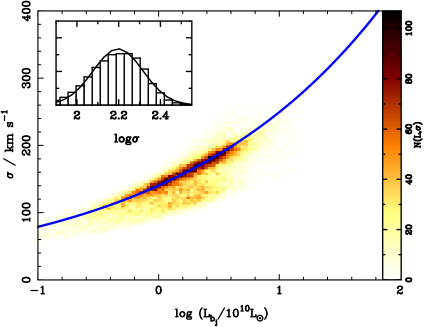
Figure 3: The Faber-Jackson relation: the number of galaxies in the mock catalogue as a function of $L$ and $\sigma$ are shown, with the blue line showing the best-fit observed relation $\sigma=\sigma_{*}(L/L_{*})^{0.25}$. The inset shows the distribution of velocity dispersions, $\log\sigma_{\mathrm{b}}$ in our mock 2df catalogue. The smooth line in the inset shows the observed velocity dispersion distribution in the SDSS found by Bernardi et al. (2003b).

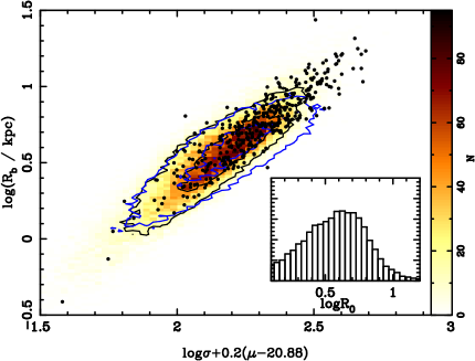
Figure 4: The fundamental plane for galaxies in the mock catalogue: the number of galaxies in the mock as a function of $R_{\mathrm{b}}$ and a combination of velocity dispersion and surface brightness. The blue contours show the same for the sample of elliptical galaxies in the SDSS (Bernardi et al., 2003b). The histogram in the inset shows the distribution of $\log{R_{\mathrm{b}}}$ in the mock catalogue. The dots show the mock lens sample created in § 4.

We show the Faber-Jackson relation and the histograms of the distributions of the velocity dispersion and bulge size in Figs. 3 & 4 for the mock catalogue. These plots show that, using only the observed $R_{\mathrm{b}}-L$ relation as input, we recover the observed Faber-Jackson relation and the fundamental plane. Of particular importance is the fact that we recover the observed velocity dispersion distribution measured for early-type galaxies by the SDSS. We conclude therefore that our mock galaxies are realistic.

These structural parameters are then used to model the bulge component in the lens as a de Vaucouleur profile (de Vaucouleurs, 1948),

$$\Sigma_{\mathrm{b}}=\Sigma_{0,\mathrm{b}}\times\exp{-(r/r_{\mathrm{s}})^{1/4}},$$ (13)

where $r_{s}=3681\times R_{\mathrm{b}}\times 0.551$ and $\Sigma_{0,\mathrm{b}}=\Gamma L/8\pi\times 5040r_{\mathrm{s}}^{2}\sqrt{1-e^{2}}$, measured in $\mathrm{kpc}$ and $\mathrm{M_{\odot}kpc^{-2}}$ respectively, and where $\Gamma$ is the fixed mass-to-light ratio of bulges taken to be $7M_{\odot}/L_{\odot}$ in the B-band. We also allow for ellipticity, $e$, in the bulge. To assign ellipticities to the bulge component in our mock galaxy catalogue, we draw an ellipticity randomly from a Gaussian distribution of mean $\bar{e}=0.3$ and standard deviation, $\sigma_{e}=0.3$, consistent with the observed ellipticities of early-type galaxies (Jorgensen & Franx, 1994).

2.3.4 Disc component

In the semi-analytic models of galaxy formation every galaxy, irrespective of morphology, also contains a disc component. The infall and merger history of haloes determines the disc properties: total disc mass, $M_{\mathrm{d}}=\Gamma L_{\mathrm{d}}$ and disc size, $R_{\mathrm{d}}$. The mass distribution of discs is taken to be well-fit by an exponential:

$$\Sigma_{\mathrm{d}}=\Sigma_{0}\exp{(-r/R_{\mathrm{d}})},$$ (14)

where $\Sigma_{0}=M_{\mathrm{d}}/\pi R_{\mathrm{d}}^{2}$ is the central surface mass density of the disc.

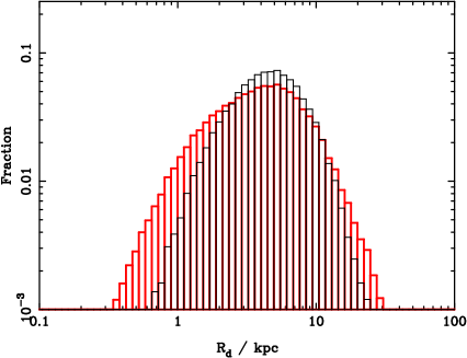
Figure 5: The distribution of disc sizes in the mock 2dF catalogue. The histograms show the distribution of $\log R_{\mathrm{d}}$ in the mock, the thick, red is for all galaxies and thin, black is for spiral galaxies only. Note that both histograms have been normalised independently.

We plot the distributions of the structural disc parameters for the mock catalogue in Fig. 5. Identifying the maximum velocity dispersion $V_{\mathrm{max}}$ of the DM halo with the disc rotational velocity, $v_{\mathrm{c}}$ also gives the Tully-Fisher relation for galaxies in our mock catalogue (see Fig. 6).

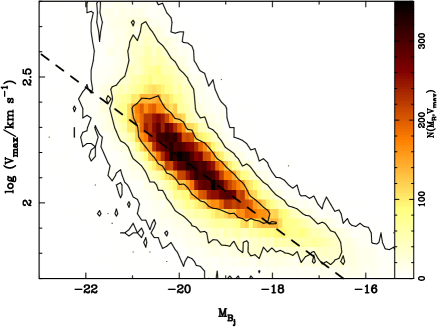
Figure 6: The distribution of number of galaxies as a function of $V_{\mathrm{max}}$ and disc luminosity in the mock catalogue. The dashed line shows the observed Tully-Fisher relation, $M_{\mathrm{B_{\mathrm{j}}}}=-4.125-7.27\times\log{V_{\mathrm{max}}}$(Tully & Fisher, 1977; Pierce & Tully, 1992; Tully & Pierce, 2000).

The blue line in Fig. 6 shows the Tully-Fisher relation observed by Tully & Pierce (2000) and Pierce & Tully (1992). There is a very good match between observed and predicted relation for $M_{\mathrm{B_{j}}}\mathrel{\hbox{\hbox to0.0pt{\hbox{\lower 4.0pt\hbox{$\sim$}}\hss}\hbox{$>$}}}-21$, corresponding to $L\mathrel{\hbox{\hbox to0.0pt{\hbox{\lower 4.0pt\hbox{$\sim$}}\hss}\hbox{$<$}}}2.15\times 10^{10}L_{\odot}$. At higher luminosities, there is an upturn in the predicted relation. Given the small observed number of objects with measured rotational velocities at these luminosities this is consistent with observational data at the present time.

2.4 Lensing properties of the composite model

To illustrate the general lensing properties of the composite mass model used, we show the image and source magnification maps of the dark matter+bulge+disc models in

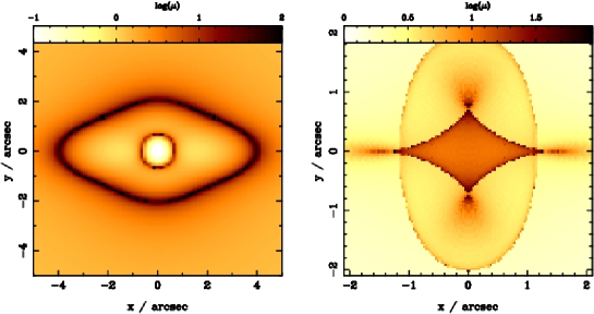
Figure 7: The image (left) and source (right) magnification maps for dark matter+bulge+disc model of a luminous $L=1.8\times 10^{11}L_{\odot}$ galaxy. The colour scale shows the magnification of a point source as a function of image and source position respectively. The source plane is at $z_{\mathrm{s}}=1$ and the image plane is at $z=0.15$. The lens has a bulge to total mass ratio B/T of $0.2$, a bulge ellipticity of $e=0.4$ and a disc inclination angle of $\theta=70\,\deg$. The dark halo mass is $M_{\mathrm{vir}}=1.3\times 10^{13}M_{\odot}$ inside $R_{\mathrm{vir}}=455\,\mathrm{kpc}$, with a concentration parameter of $c=9$.

Fig. 7 for a spiral galaxy with $L=10^{11}L_{\odot}$. Note the strong asymmetry introduced by the disc component. This is expected since for inclination angles of $\theta>65\,\deg$, the projected surface mass density along the major axis is strongly increased for thin discs (Möller & Blain, 1998).

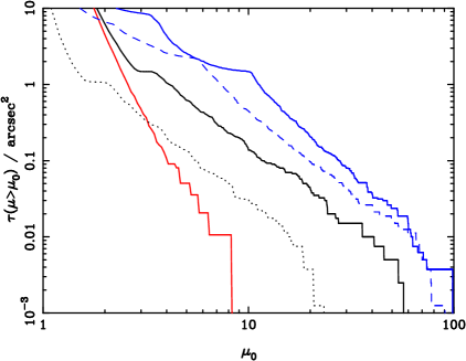
Figure 8: The lensing cross section as a function of magnification $\mu$ for DM, DM+bulge and DM+bulge+disc models of a typical $L=10^{11}L_{\odot}$ galaxy in the mock catalogue. Cumulative histograms of the cross sectional area for lensing of point sources by magnifications of more than $\mu_{0}$, $\tau(\mu>\mu_{0})$ are shown. The solid, red line is for the pure DM model. The solid, black line shows the result of adding a bulge and the solid blue line is for the complete DM+bulge+disc model. The dashed black and blue lines show the magnification cross sections for model of bulge and bulge+disc without dark matter, respectively. Model parameters are as for the previous figure.

The magnification curves in the source and image planes are shown in Fig. 8. The NFW dark matter profile on its own does not have a significant lensing cross section in this example, as the concentration parameter $c$ of the dark matter halo is too low. It is interesting to note, however, that despite this the magnification cross sections for the composite model are influenced significantly by the DM component. This can be seen by comparing the lensing cross-sections as a function of magnification shown as solid (DM) and dashed (no DM) lines in Fig. 8. The cross section for the case with no DM is a factor of $\sim 2$ below that with DM, for almost all magnifications above about 3. Therefore, even in cases when the DM halo is not concentrated enough to produce lensing, it still affects the lensing cross section significantly.

3 The expected lens properties of the galaxy population in the 2dF

3.1 Calculation of lensing properties

Once each galaxy has been assigned a NFW halo+bulge+disc mass model, the calculation of the lensing probability for a given source population depends only on the geometric parameters, i.e. the redshifts of the source, lens and the cosmological parameters. We are not interested in constraining cosmological parameters with lensing in this work and we fix the underlying cosmology as described in § 1.

We calculate the lensing properties of each of the $\sim 70,000$ galaxies in the mock catalogue using ray-tracing. Since we consider only one lens plane, this reduces to numerically solving the lens equation,

$$\bf{\theta}=\bf{\beta}-\bf{\alpha},$$ (15)

where $\bf{\theta}$ is the imaged position of a source at angular position $\bf{\beta}$ and $\bf{\alpha}$ is the deflection angle.

For the calculations in this section, we fix the sources at $z_{\mathrm{source}}=1$. In order to allow ray-tracing calculations of sufficient accuracy in a reasonable amount of time we use the adaptive grid technique, as described in Möller & Blain (2001). For each galaxy, an approximate lensing region size is determined using the extent of the Einstein radius. This is done by finding the points in the image plane at which the magnification diverges. The physical size of the putative lensing region is then set to $20$ times the distance of the most distant such points to the galaxy, giving a conservative upper estimate of the region within which multiple imaging can occur. This region in the image plane is then covered with an initial grid of $40\times 40$ rectangles. Each grid point is then mapped to the source plane. After mapping, magnifications on the image plane are given by the ratio of the areas of the original to that of the mapped rectangles. Depending on the magnification $\mu$ the initial grid is then adaptively refined by subdividing each rectangle into $n_{\mathrm{sub}}$ smaller rectangles, with $n_{\mathrm{sub}}(\mu)=1+(\mu-5)/195\times 20$, for $\mu>5$, and with no refinement otherwise. This resulting adaptive grid is then also mapped onto the source plane. Finally, the image magnifications and image multiplicities are calculated on the resulting fine grid on the source plane.

3.2 Total lensing cross sections and image separation distributions

Two statistics have been used in the past to constrain cosmological parameters (Chae, 2003; Kochanek, 1993) and lens galaxy population properties (Chae, 2005; Kochanek, 1996): total lensing cross sections and image separation distributions. The total lensing cross section we obtain from our mock catalogue is $100752\,\mathrm{arcsec}^{2}$ in a total survey area of $657\deg^{2}$, with 79042 galaxies below redshift of 0.2 constituting our lens galaxy population. This gives a total probability of a source being lensed as $1.13\times 10^{-5}$. This estimate neglects magnification bias and we show in § 4 that magnification bias increases the lensing probability dramatically.

We plot the lensing cross section for our mock catalogue as a function of lens galaxy luminosity and halo virial mass in

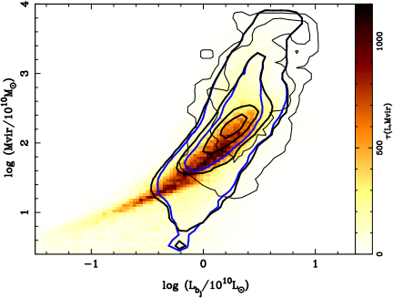
Figure 9: The lensing cross section as function of luminosity and mass. The colour scale shows the distribution of all galaxies as a function of $L$ and $M_{\mathrm{vir}}$. The blue contour shows the lensing cross section distribution for the complete DM+bulge+disc models. The thick, black contour shows the cross section for DM+bulge models and the thin black contours are for DM only models. The contour levels are $100$, $300$, $700$ and $1000\,\mathrm{arcsec}^{2}$ for the first two cases and $0.1$, $1$ and $10\,\mathrm{arcsec}^{2}$ in the latter case.

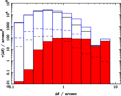
Figure 10: The expected image separations in the 2dF. As in the previous figure, we show the results for the DM only (red), the DM+bulge but no disc (black) and the DM+bulge+disc (blue) models. The solid lines correspond to the image separation histogram of 2 image systems, the dotted line shows the maximum image separation for 4 image systems. In all cases, shown above the effect of magnification bias is not included.

Fig. 9. The contours show the lensing cross section for background sources at $z_{\mathrm{source}}=1$ as a function of mass, $M_{\mathrm{vir}}$ and luminosity $L_{\mathrm{B_{j}}}$. Comparison with the underlying distribution for all galaxies in the sample shows that the contribution to strong lensing cross section comes preferentially from massive, luminous galaxies. The shift in the luminosity from a peak luminosity of $L^{\mathrm{peak}}_{\mathrm{tot}}\sim 10^{10}L_{\odot}$ for the total distribution to a peak of $L^{\mathrm{peak}}_{\mathrm{lens}}=2\times 10^{10}L_{\odot}$ for the lensing sample is clearly strong. An additional shift to higher virial masses by a factor of $\sim 2$ is also evident. The baryonic component dominates the lensing cross section of galaxies, but, for a fixed luminosity, the contribution of high mass objects to the lensing cross section is larger. The dark matter component therefore also plays a key role. In Fig. 10 we show the expected distribution of image separations. Here, we clearly see the relative effects of the various lens components. For small image separations (corresponding to low masses) the cross section is completely dominated by the baryonic component. Large image separation systems, mainly corresponding to groups and clusters, have lensing cross sections that depend much more on the dark matter content.

It is clear from these plots that the baryonic component is absolutely crucial in determining statistical lensing properties on galaxy scales. The importance of the baryonic contribution to the lensing cross sections of DM haloes is clearly seen: it increases by a factor of $10-1000$ for systems with image separations between $\sim 0.1$ and $\sim 1\,\arcsec$. The increase is smaller for systems with large image separations. These systems correspond to lensing by massive central cluster and group galaxies. As the Einstein radius increases for more massive systems, the fraction of DM within the Einstein radius also increases, due to the shallower slope of the DM component. Despite this importance of the baryonic component, the lensing cross section at a fixed $L$ does depend on the DM halo mass, $M_{\mathrm{vir}}$, even for highly luminous galaxies (cf. Fig. 8).

3.3 Image geometries: two and four image systems

Previous work by e.g. Möller & Blain (1998) and Blain (1998) has shown that baryonic components can significantly change the total lensing cross section. The disc component plays a major role in this; inclined discs can increase the lensing cross section significantly. However, as suggested by Möller et al. (2003) this effect is important only for late-type systems, whereas early-type galaxies have too small a disc component to change the lensing cross section significantly. The ratio of 4 to 2 image systems , however, may be affected strongly, as even relatively low mass discs can increase the asymmetry of the lensing potential noticeably.

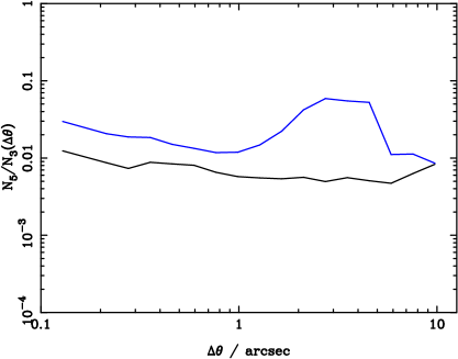
Figure 11: The average ratio of the lensing cross section for 4: 2 image-systems as a function of image separation. The black line is for a DM+bulge only model for all galaxies in the mock catalogue, and the blue line for a DM+bulge+disc model. Magnification bias is not included in this calculation.

We show the ratio of 4 to 2 image systems in the catalogue for the DM+bulge and the DM+bulge+disc models in Fig. 11. For systems with $10^{11}L_{\odot}\mathrel{\hbox{\hbox to0.0pt{\hbox{\lower 4.0pt\hbox{$\sim$}}\hss}\hbox{$<$}}}L\mathrel{\hbox{\hbox to0.0pt{\hbox{\lower 4.0pt\hbox{$\sim$}}\hss}\hbox{$<$}}}10^{12}L_{\odot}$ the fraction of late-type galaxies is high enough to increase the cross section for 4-image systems by more than a factor of $\sim 10$. Again, this result neglects the effect of magnification bias. Magnification bias is expected to favour late-type galaxies as 4-image lens systems, given that the expected cross section for magnification of $\mu\sim 10-20$ is a factor of up to $\sim 10$ larger for inclined spiral lenses (Möller & Blain, 1998). However, as we show in § 4, this is not the case: elliptical galaxies have a smaller cross-sectional area for magnifications in that range, but they generally have a larger cross section for magnifications above $20$. This implies that magnification bias in fact favours the moderately elliptical gravitational potential of early-type galaxies.

3.4 Selection biases

The results presented above do not include the effects of selection biases. All surveys are by construction limited in flux, resolution or some other observational criteria. These varied selections can strongly affect the inferred properties of lens samples. A flux limited survey for example, will be strongly affected by magnification bias for sources with a steep luminosity function. Since galaxies and radio sources follow quite steep luminosity functions magnification bias is important for lensing in the radio as well as in the optical. One can estimate the effect of magnification bias for simple selection criteria. The cumulative probability distribution function for magnification above a value $A$ is generally $P(\mu>A)\propto A^{-\alpha}$, where $\alpha=2$ for SIS lenses. Assuming that the probability that a source enters the survey is 1 for $\mu\times F>F_{0}$ and 0 otherwise, it follows that the fraction of sources of luminosity $F$ that are observed at flux $F^{\prime}$ is $N(F^{\prime})=\int_{0}^{\infty}dP/dA(A)N(F^{\prime}/A)dA$ [cf. Maoz et al. (1993) and King & Browne (1996)]. For a lens population with a more complicated lens model, an analytic calculation of the effect of magnification bias becomes infeasible. Including the selection effects due to finite resolution limits requires a numerical calculation – which we describe in the next section.

4 A mock sample of lens systems

We use the lensing code gLens together with our mock galaxy catalogue to create a sample of lens systems, including observational selection effects. We include two key selection effects: a flux limit and a resolution limit. Concentrating on lensed radio sources, we create a sample that has selection criteria in concordance with the CLASS survey (Chae, 2003):

1. The total flux F of each system of images is above $F_{0}$,

2. the image separation is $>0.03\arcsec$,

3. and for double image systems the magnification ratio of bright to faint image is $>0.1$.

We create the sample using rough estimates of the lensing cross section for each galaxy assuming spherical symmetry, by solving the lens equation for the approximate Einstein radius, $\theta_{\mathrm{er}}$. We then populate the total estimated cross section area, $A_{\mathrm{attempt}}$ with $N_{\mathrm{attempt}}$ sources. For each source, we pick a random flux from a distribution $N\propto F^{-2.1}$ and assign a source redshift from a redshift distribution that is a Gaussian with mean $\bar{z_{\mathrm{s}}}=1.27$ and width $0.95$ as found by Willott et al. (2001) in the 6CE and 7CRS radio samples. For each source, we find the positions of the images using an adaptive lensing technique similar to the one described in Wucknitz (2004). We then apply the selection criteria (i)-(iii) to the lens system. If the system satisfies all these criteria, it is included in the lens sample, otherwise another foreground galaxy and source pair are selected randomly until the desired number of lens systems is obtained. For a number of $N_{\mathrm{attempt}}$ ‘trial’ sources, placed in an area $A_{\mathrm{attempt}}<<A_{\mathrm{survey}}$ where $A_{\mathrm{survey}}$ is the total area of the survey, there is a number of $N_{\mathrm{unlensed}}$ sources that are unlensed but above the flux limit for detection. The number of expected lenses in the survey is then given by $N_{\mathrm{lens}}=f_{\mathrm{lens}}N_{\mathrm{unlensed}}\times A_{\mathrm{survey}}/A_{\mathrm{attemps}}$, with $f_{\mathrm{lens}}$ being the lensing fraction.

4.1 Properties of the lens sample

We use the procedure described above, to create a sample of $N_{\mathrm{lens}}=400$ lens systems from our mock galaxy catalogue. This number of lens systems was chosen to obtain a reasonable statistical sample while keeping the time needed for computations tractable. The total number of ‘trial’ sources was $N_{\mathrm{attempt}}=110000$ in a total area of $A_{\mathrm{attempt}}=0.1384\deg^{2}$. Of these ‘trial’ sources, a number $N_{\mathrm{unlensed}}=60\pm 7$ were unlensed but above the detection flux limit $F_{0}$. The total number of sources in the total area of $A_{\mathrm{survey}}=651\deg^{2}$ that would create 400 lenses is $282021$, yielding a fraction of $f_{\mathrm{lens}}=1.4\pm 0.18\times 10^{-3}$ of all ‘observed’ sources as lensed. This fraction is in good agreement with the lens fraction observed in CLASS.

4.1.1 Lens velocity dispersions and morphologies

We determine the average velocity dispersion of the $400$ mock lens systems to be $\bar{\sigma}=164.2\pm 2.6\,\mathrm{km\,s^{-1}}$. This value is consistent with but slightly lower (by about $5\,\mathrm{km\,s^{-1}}$) than what is observed in the CLASS survey.

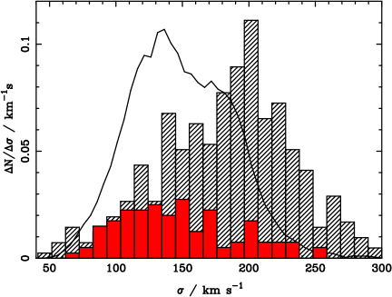
Figure 12: The distribution of lens velocity dispersion in a mock lens sample selected in the radio. The black, hatched histogram shows the velocity dispersion distribution of all lens systems with an average velocity dispersion of $\bar{\sigma}=164.2\pm 2.6\,\mathrm{km\,s^{-1}}$, with the majority of lens galaxies ($\sim 80\%$) being ellipticals. The red, filled histogram shows the statistics for 4 image lenses only. The solid, thin black line shows the distribution of velocity dispersions of all ellipticals in our mock 2dF catalogue.

The distribution of lens velocity dispersions for 2dF lenses expected in a radio selected survey is shown in Fig. 12. The distribution for all systems (black) and for 4-image systems only (red) is shown. We also show the location of lens galaxies in the sample in Fig. 4 in § 2.3.3 (black dots). Even though the lenses lie on the fundamental plane, the complete sample of lens systems has a significantly higher velocity dispersion than the elliptical galaxy population as a whole. However, the velocity dispersion function for 4-image lenses follows the distribution of the galaxy velocity dispersion for all galaxies much more closely. In the complete sample, a total fraction of about $80\pm 5\%$ of lenses are ellipticals with a bulge-to-total light ratio of $>0.6$. This fraction decreases to $70\pm 10\%$ for the 4-image system subsample. The fact that these two fractions are very similar suggests that magnification bias is stronger for early-type massive galaxies with a moderately asymmetric potential, rather than less massive late-type systems with strong ellipticity in the potential due to a massive disc.

4.1.2 Image separations and image geometries

Using the above selection criteria, we find that the average image separation is $\bar{\Delta\theta_{\mathrm{max}}}=3.3\pm 0.2\arcsec$. Taking into account the expected difference in redshift distributions of the lenses, $\bar{z}\sim 0.1$ and $\bar{z_{\mathrm{CLASS}}}\sim 0.4$, and noting that the image separations scale as $\Delta\theta_{\mathrm{max}}\propto D_{\mathrm{LS}}/D_{\mathrm{OS}}$ this compares well with the observed image separations in the CLASS sample $\Delta\theta_{\mathrm{CLASS}}=1.13\arcsec$.

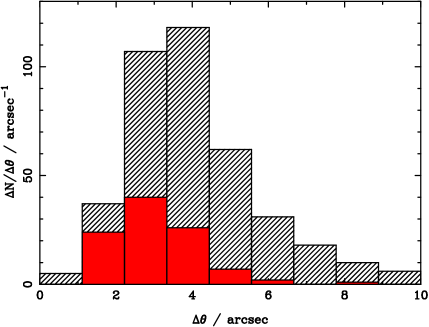
Figure 13: The expected distribution of image separations in a radio selected survey for 2dF lenses. As in the previous figure, the black hatched area shows the histogram for all lens systems. The red, solid region shows the statistics of 4 image systems only. In contrast to Fig. 10 in § 3, this calculation includes magnification bias.

The distribution of image separations produced by 2dF lenses expected in a radio selected survey is shown in Fig. 13. We also show the image separation statistic for a subsample consisting of 4-image systems. The average maximum image separation decreases to $\bar{\Delta\theta}=2.57\pm 0.6\arcsec$ when only 4-image systems are considered. Our model for lenses in the 2dF predicts a fraction of $70\pm 5\%$ of double image systems, with a fraction of $\sim 30\pm 5\%$ being lens systems with four images. Depending on the particular choice of known lens systems to compare with, these numbers are consistent/inconsistent with observations. The sample used by Rusin & Tegmark (2001) contains seven quadruples and five doubles, whereas the sample used by Chae (2003) and Chae (2005) contain ten lenses with four quadruple image systems. These samples differ in their selection criteria, and since the number of known lens systems is low it is difficult to draw any firm conclusions. From our analysis, it does appear that the number of observed quadruple systems is slightly higher than what would be expected, even if we compare with the sample of Chae (2005). Since our model includes ellipticities and disc components it is difficult to explain any further asymmetry in the lensing potential needed to increase the fraction of quadruples with anything other than the presence of other mass concentrations in the vicinity of the primary lens. These environmental effects are discussed in more detail in Möller (2006).

5 Discussion and conclusions

Surveys, like the 2dF and the SDSS are likely to contain a large number of gravitational lens systems. We predict the number of lenses and lensing statistics expected in the 2dF survey. The number of observed lensing systems is a function of the statistical properties of the foreground galaxy population, the source population, selection biases and cosmological parameters. Taking the cosmological parameters as known we calculate the expected lensing statistics for point sources at a fixed redshift using realistic multi-component galaxy models. Our fiducial galaxy consists of an NFW halo, an elliptical bulge and an inclined disc. Detailed galaxy properties are predicted using semi-analytic modeling of galaxies in the Millennium Run, currently the largest available N-body simulation. Using ray-tracing techniques in combination with the galaxy model we predict the statistical lensing properties of large surveys with realistic galaxy lens models.

We calculate the lensing cross section for a complete sample of 70,000 galaxies at redshifts of $z_{\mathrm{lens}}<0.2$ that fulfill the selection criteria of the 2dF survey. With background sources at a fixed redshift of $z_{\mathrm{source}}=1$ we demonstrate that the main contribution to the lensing cross section comes from the baryonic component of luminous, early-type galaxies. It is important to note here that this does not mean that the lensing cross section is insensitive to the DM component in these galaxies. In fact the distribution of galaxy masses at a fixed luminosity, $n(M_{\mathrm{vir}}|L)$ for a lens sample is different from that for the complete population of early-type galaxies. As shown in Fig. 9 – the mass function of lenses peaks at a value that is a factor of about 2 higher than the overall galaxy sample. If magnification bias is not included, we find that, for systems with maximal image separations between $1-3\arcsec$, the disc component of spirals increases the lensing cross section by a factor of $\sim 10$. This shows that disc components of spirals are an important contribution to statistical lensing calculations. However, when we do include magnification bias we found that this effect is weaker due to a trade-off between increase in cross section for late-type galaxies on the one hand, and a much stronger magnification bias for four image geometries in moderately elliptical massive galaxies on the other (cf. discussion in § 3.3 and § 4.1.1).

To make firm predictions with clear selection criteria we simulate a sample of 400 radio selected lens systems that fulfill the CLASS selection criteria in terms of flux and magnification ratios. We find that, in surveys like the 2dF or SDSS, including magnification bias, about $1.4\times 10^{-3}$ of all background radio sources are lensed by galaxies within the survey. This number is fairly independent of the inclusion of a disc component, but does depend crucially on the presence of the baryonic bulge, and even more strongly, on the magnification bias. The number of lenses per observed source increases from $1.1\times 10^{-5}$ without magnification bias to $1.4\times 10^{-3}$ including the effect of magnification bias. Using our model we also calculate the relative incidence of 4 and 2 image systems. The inferred fraction of $30\pm 5\%$ of quadruple systems is consistent with observed values.

The key result of our work is that samples of lens galaxies expected in surveys like the 2dF and the SDSS distinguish themselves from the overall galaxy population in several important ways:

• A fraction of $\sim 80\%$ of lenses are expected to be of early-type morphologies, compared to only $\sim 35\%$ in the overall galaxy sample. This number is reduced slightly if only four image systems are considered.

• The average velocity dispersion of lensing galaxies is $\bar{\sigma}=165\,\mathrm{km\,s^{-1}}$ as opposed to $150\,\mathrm{km\,s^{-1}}$ for all early-type galaxies. Furthermore, the distribution is dramatically different – the distribution for lens galaxies has a maximum at $\sigma\sim 200\,\mathrm{km\,s^{-1}}$, with a long tail towards lower velocity dispersions.

• The peak of the luminosity distribution of lens galaxies is a factor of $\sim 2$ higher than that of the total galaxy population.

• For a given luminosity, lens galaxies reside in haloes that are more massive by a factor of $\sim 2$ on average than the overall sample of ellipticals.

Interestingly, we also find that the properties of the lens sample differ depending on whether 4 or 2 image systems are considered. Initially surprising is the result that 4-image systems tend to have lower velocity dispersions; they trace the velocity dispersion distribution of the overall early-type galaxy population much better. This can be explained by noting that the asymmetries in the potential have a larger effect for lower mass galaxies – the ratio of 4: 2 image systems is therefore expected to be much higher for galaxies with lower velocity dispersions. In addition, the predominant cause for 4-image lens geometries is a modest ellipticity in the potential, which is more likely to be created by moderately inclined discs, and hence by later-type galaxies which tend to have lower velocity dispersions. Our assumption that asymmetries in the potential are due to the baryonic components and that the dark matter haloes are spherical may also affect this result. However, since lens galaxies in the catalogue are dominated strongly by the baryonic component, this should not change the statistics significantly.

All these differences between lens samples and the underlying galaxy population are very important to understand if lensing studies are to be used to obtain a better understanding of the galaxy evolution. This holds both for statistical studies but also for studies of individual systems. For example, single cases of lenses for which the mass distribution is steeper than the average profile predicted by simulations at the same mass do not point to any inconsistency; it is absolutely crucial that the full predicted distribution functions are considered. Our statistical analysis demonstrates clearly that lensing galaxies are a biased population. They preferentially sample the high mass end of all galaxies. This systematic, in fact, limits the unbiased study of galaxy evolution using a sample of lensing galaxies (Mitchell et al., 2005; Ofek et al., 2003).

In our analysis we do not examine the effect of the environment. In a recent study by Oguri (2006) it has been shown that the presence of other mass concentrations in the vicinity can increase the lensing cross sections for high image separations by several tens of percent. Interestingly, this result was also previously found by Turner et al. (1984) who used a very simple mass-sheet model to calculate the effect of environment. We address the effect of environment, and in particular the incidence and statistical properties of lens galaxies in groups in a subsequent publication. It is worthwhile to note here, that for low redshifts, the environment is expected to have a much smaller effect, as the ratio between expected image separations of galaxy lenses and the typical distance to nearby galaxies is much smaller at lower redshifts (at $z\sim 0.05$ a distance of $1\arcsec$ corresponds to about 1 kpc, at $z\sim 0.5$ to about 6 kpc).

Our calculations show that selection effects, and in particular magnification biases, have a strong effect on lens statistics. Given that magnification bias is important, it does appear that the distribution of the sources may also strongly influence lensing statistics. For radio selected samples the selection criteria can be defined clearly and the source luminosity function is known to an adequate degree to predict lensing statistics reasonably well. In the optical or infrared, however, both selection criteria and source properties are not as well understood. To use lenses selected at these wavelengths in a statistical way requires careful analysis to disentangle the various effects, like source luminosity functions, magnification bias and source redshift distributions. Simulating real imaging data in various wave-bands will be needed to test the particular predictions of a given model of the lens and source population.

The basis for this study has been to use one of the best models of galaxy formation currently available and test the predicted lensing properties of such a sample. Our choice of a semi-analytic model was motivated strongly by the advantage that the relation between luminous and the DM is predicted in a way that is self-consistent, easy to interpret and use. It is important to point out, though, that these models do have limitations. Even though the predictions at low redshift appear to be consistent with observations, it is not clear if current semi-analytic models predict all the observed properties of galaxies at higher redshifts correctly. It is encouraging for semi-analytic models that our results are consistent with the current known statistical lens sample, but we add the caveat that the known lens sample is small. Testing models of galaxy formation and evolution using strong lensing statistics seems a promising approach; future lens surveys will increase the number of lens systems known by a large number and if the selection criteria in these surveys can be understood, much can be learnt about the relation between mass and light on galaxy scales.

6 Summary

We predict the lensing properties of galaxies in low-redshift surveys with $z\mathrel{\hbox{\hbox to0.0pt{\hbox{\lower 4.0pt\hbox{$\sim$}}\hss}\hbox{$<$}}}0.2$ using realistic galaxy mass models based on a recent semi-analytic simulation of galaxies formation within the Millennium Run N-body simulation. Using ray-tracing techniques we calculate the lensing cross section for 2 and 4 image systems for a multi-component lens model consisting of a DM halo, a bulge and a disc component. Our key results can be summarised as follows:

• The predicted lensing rate for radio sources in low redshift surveys like the 2dF is $1.4\times 10^{-3}$.

• A fraction of $80\pm 5\%$ of all lens galaxies are predicted to be ellipticals.

• The predicted average maximum image separation is $3.3\pm 0.2\,\mathrm{arcsec}$.

• The average velocity dispersion of lenses is $\bar{\sigma}=164\pm 2.6\,\mathrm{km\,s^{-1}}$.

• The baryonic component is the most important contributor to the lensing cross sections for galaxy scale masses, but the dark matter distribution also affects the lensing statistics of composite lens models significantly.

• Lens galaxies are more luminous and, for a fixed luminosity, reside in dark matter haloes that have masses a factor of 2 higher than the overall galaxy population.

• The velocity dispersion distribution of lens galaxies is shifted to significantly higher values of the velocity dispersion with respect to that of a complete sample of galaxies.

• Four image systems have, on average, a lower velocity dispersion, a later type morphology and a lower average maximum image separation than double image systems.

Our quantitative predictions are entirely consistent with the statistics in the CLASS survey. We pioneer the use of detailed semi-analytic models of galaxies to predict statistical lensing properties. This approach provides testable predictions for the lensing statistics and conversely, statistical lensing can provide useful constraints on galaxy formation models in the near future. In ongoing work we address in detail the effect of environment for lensing statistics.

References

- Adelman-McCarthy et al. (2006) Adelman-McCarthy J. K., et al., 2006, ApJS, 162, 38
- Bartelmann et al. (1998) Bartelmann M., Huss A., Colberg J. M., Jenkins A., Pearce F. R., 1998, A&A, 330, 1
- Bernardi et al. (2003a) Bernardi M., et al., 2003a, AJ, 125, 1866
- Bernardi et al. (2003b) Bernardi M., et al., 2003b, AJ, 125, 1817
- Blain (1998) Blain A. W., 1998, MNRAS, 295, 92
- Bower et al. (2006) Bower R. G., Benson A. J., Malbon R., Helly J. C., Frenk C. S., Baugh C. M., Cole S., Lacey C. G., 2006, MNRAS, 659
- Broadhurst et al. (2005) Broadhurst T., Benítez N., Coe D., Sharon K., Zekser K., White R., Ford H., Bouwens R., Blakeslee J., Clampin, 2005, ApJ, 621, 53
- Bullock et al. (2001) Bullock J. S., Kolatt T. S., Sigad Y., Somerville R. S., Kravtsov A. V., Klypin A. A., Primack J. R., Dekel A., 2001, MNRAS, 321, 559
- Cappellari et al. (2006) Cappellari et al., 2006, MNRAS, 366, 1126
- Chae (2003) Chae K.-H., 2003, MNRAS, 346, 746
- Chae (2005) Cahe K.-H., 2005, ApJ, 630, 764
- Cohn et al. (2001) Cohn J. D., Kochanek C. S., McLeod B. A., Keeton C. R., 2001, ApJ, 554, 1216
- Colless et al. (2001) Colless M., et al., 2001, MNRAS, 328, 1039
- Cooray & Cen (2005) Cooray A., Cen R., 2005, ApJL, 633, L69
- Croton et al. (2006) Croton et al., 2006, MNRAS, 365, 11
- Dalal et al. (2005) Dalal N., Hennawi J., Bode P., 2005, ApJ, 622, 99
- de Jong et al. (2004) de Jong R. S., Simard L., Davies R. L., Saglia R. P., Burstein D., Colless M., McMahan R., Wegner G., 2004, MNRAS, 355, 1155
- de Vaucouleurs (1948) de Vaucouleurs G., 1948, Annales d’Astrophysique, 11, 247
- Eke et al. (2001) Eke V. R., Navarro J. F., Steinmetz M., 2001, ApJ, 554, 114
- Ferreras et al. (2005) Ferreras I., Saha P., Williams L. L. R., 2005, ApJL, 623, L5
- Fukugita et al. (1992) Fukugita M., Futamase T., Kasai M., Turner E. L., 1992, ApJ, 393, 3
- Gerhard et al. (2001) Gerhard O., Kronawitter A., Saglia R. P., Bender R., 2001, AJ, 121, 1936
- Helbig et al. (1999) Helbig P., Marlow D., Quast R., Wilkinson P. N., Browne I. W. A., Koopmans L. V. E., 1999, A&A Supp, 136, 297
- Huterer et al. (2005) Huterer D., Keeton C. R., Ma C.-P., 2005, ApJ, 624, 34
- Jorgensen & Franx (1994) Jorgensen I., Franx M., 1994, ApJ, 433, 553
- Kauffmann et al. (1993) Kauffmann G., White S. D. M., Guiderdoni B., 1993, MNRAS, 264, 201
- Kauffmann et al. (2004) Kauffmann G., White S. D. M., Heckman T. M., Ménard B., Brinchmann J., Charlot S., Tremonti C., Brinkmann J., 2004, MNRAS, 353, 713
- Keeton & Zabludoff (2004) Keeton C. R., Zabludoff A. I., 2004, ApJ, 612, 660
- King & Browne (1996) King L. J., Browne I. W. A., 1996, MNRAS, 282, 67
- Kneib et al. (2003) Kneib J.-P., Hudelot P., Ellis R. S., Treu T., Smith G. P., Marshall P., Czoske O., Smail I., Natarajan P., 2003, ApJ, 598, 804
- Kochanek (1993) Kochanek C. S., 1993, MNRAS, 261, 453
- Kochanek (1996) Kochanek C. S., 1996, ApJ, 473, 595
- Koopmans & Treu (2002) Koopmans L. . V. E., Treu T., 2002, ApJL, 568, L5
- Koopmans & Treu (2003) Koopmans L. V. E., Treu T., 2003, ApJ, 583, 606
- Kundic et al. (1997a) Kundic T., Hogg D. W., Blandford R. D., Cohen J. G., Lubin L. M., Larkin J. E., 1997a, AJ, 114, 2276
- Kundic et al. (1997b) Kundic T., et al., 1997b, ApJ, 482, 75
- Maoz et al. (1993) Maoz D., et al. , 1993, ApJ, 409, 28
- Meneghetti et al. (2005) Meneghetti M., Jain B., Bartelmann M., Dolag K., 2005, MNRAS, 362, 1301
- Mitchell et al. (2005) Mitchell J. L., Keeton C. R., Frieman J. A., Sheth R. K., 2005, ApJ, 622, 81
- Möller & Blain (1998) Möller O., Blain A. W., 1998, MNRAS, 299, 845
- Möller & Blain (2001) Möller, O., Blain A. W., 2001, MNRAS, 327, 339
- Möller et al. (2003) Möller O., Hewett P., Blain A. W., 2003, MNRAS, 345, 1
- Möller et al. (2002) Möller O., Natarajan P., Kneib J.-P., Blain A. W., 2002, ApJ, 573, 562
- Möller (2006) Möller O. e. a., 2006, Lensing by groups in 2df and sdss, MNRAS, in preparation
- Navarro et al. (1997) Navarro J. F., Frenk C. S., White S. D. M., 1997, ApJ, 490, 493
- Norberg et al. (2002) Norberg P., et al., 2002, MNRAS, 336, 907
- Ofek et al. (2003) Ofek E. O., Rix H.-W., Maoz D., 2003, MNRAS, 343, 639
- Oguri (2006) Oguri M., 2006, MNRAS, 227
- Oguri et al. (2005) Oguri M., Keeton C. R., Dalal N., 2005, MNRAS, 364, 1451
- Pierce & Tully (1992) Pierce M. J., Tully R. B., 1992, ApJ, 387, 47
- Rhee (1991) Rhee G., 1991, Nature, 350, 211
- Rusin & Ma (2001) Rusin D., Ma C.-P., 2001, ApJL, 549, L33
- Rusin & Tegmark (2001) Rusin D., Tegmark M., 2001, ApJ, 553, 709
- Schechter et al. (1997) Schechter P. L., et al., 1997, ApJL, 475, L85+
- Somerville & Primack (1999) Somerville R. S., Primack J. R., 1999, MNRAS, 310, 1087
- Spergel et al. (2006) Spergel D. N., et al., 2006, preprint (astro-ph/0603449)
- Springel et al. (2005) Springel V., et al., 2005, Nature, 435, 629
- Treu & Koopmans (2003) Treu T., Koopmans L. V. E., 2003, MNRAS, 343, L29
- Tully & Fisher (1977) Tully R. B., Fisher J. R., 1977, A&A, 54, 661
- Tully & Pierce (2000) Tully R. B., Pierce M. J., 2000, ApJ, 533, 744
- Turner et al. (1984) Turner E. L., Ostriker J. P., Gott J. R., 1984, ApJ, 284, 1
- Vale & Ostriker (2004) Vale A., Ostriker J. P., 2004, MNRAS, 353, 189
- Willott et al. (2001) Willott C. J., Rawlings S., Blundell K. M., Lacy M., Eales S. A., 2001, MNRAS, 322, 536
- Wucknitz (2002) Wucknitz O., 2002, MNRAS, 332, 951
- Wucknitz (2004) —, 2004, MNRAS, 349, 1
- Wyithe et al. (2002) Wyithe J. S. B., Agol E., Turner E. L., Schmidt R. W., 2002, MNRAS, 330, 575
- Zhao & Qin (2003) Zhao H., Qin B., 2003, ApJ, 582, 2