Canals in Milky Way radio polarization maps

Abstract

Narrow depolarized canals are common in maps of the polarized synchrotron emission of the Milky Way. Two physical effects that can produce these canals have been identified: the presence of Faraday rotation measure ($\mathrm{RM}$) gradients in a foreground screen and the cumulative cancellation of polarization known as differential Faraday rotation. We show that the behaviour of the Stokes parameters $Q$ and $U$ in the vicinity of a canal can be used to identify its origin. In the case of canals produced by a Faraday screen we demonstrate that, if the polarization angle changes by $90\degr$ across the canal, as is observed in all fields to-date, the gradients in $\mathrm{RM}$ must be discontinuous. Shocks are an obvious source of such discontinuities and we derive a relation of the expected mean separation of canals to the abundance and Mach number of supernova driven shocks, and compare this with recent observations by Haverkorn et al. (2003). We also predict the existence of less common canals with polarization angle changes other than $90\degr$. Differential Faraday rotation can produce canals in a uniform magneto-ionic medium, but as the emitting layer becomes less uniform the canals will disappear. We show that for moderate differences in emissivity in a two-layer medium, of up to $1/2$, and for Faraday depth fluctuations of standard deviation $\lesssim 1\,\mathrm{rad}$, canals produced by differential rotation will still be visible.

1 Introduction

Polarized (synchrotron) radio emission is a rich source of information about the relativistic and thermal plasmas and magnetic fields in the interstellar medium (ISM). Recent observations have revealed an abundance of unexpected features that arise from the propagation of the emission through the turbulent ISM (Wieringa et al., 1993; Uyaniker et al., 1998; Duncan et al., 1999; Gray et al., 1999; Haverkorn et al., 2000; Gaensler et al., 2001; Wolleben et al., 2006). Arguably the most eye-catching is the pattern of depolarized canals: a random network of dark narrow regions, clearly visible against a bright polarized background. These canals evidently carry information about the ISM, but it is still not quite clear how this information can be extracted. Two theories for the origin of the canals have been proposed; both attribute the canals to the effects of Faraday rotation, but one invokes steep gradients of the Faraday rotation measure ($\mathrm{RM}$) across the telescope beam, in a Faraday screen (Haverkorn, Katgert & de Bruyn, 2000, 2004), whereas the other relies on the line-of-sight effects producing differential Faraday rotation (Beck, 1999; Shukurov & Berkhuijsen, 2003). In order to use the canal properties to derive parameters of the ISM, one must correctly identify their origin.

In this letter we briefly discuss a few important aspects of the two theories describing the origin of canals. Detailed discussion of relevant depolarization mechanisms is presented in Fletcher & Shukurov (2006a, and in preparation). Canals produced by Faraday rotation measure gradients are discussed in Section 2 where we show that these canals require a discontinuous distribution of free electrons and/or magnetic field; we further suggest an interpretation of the discontinuities in terms of interstellar shocks. The case of differential Faraday rotation is discussed in Section 3; in Section 4 we suggest an observational test that can be used to identify the specific mechanism that produces a given canal.

The defining features of the canals are as follows:

1. the observed polarized emission $P$ approaches the polarization noise level $\sigma_{P}$, $P\la\sigma_{P}$;

2. the canal is about one beam wide;

3. the canal passes through a region of significant polarized intensity, say $P\ga 3\sigma_{P}$;

4. the canal is not related to any structure in total intensity, and so cannot be readily explained by, e.g., an intervening gas or magnetic filament.

Polarized intensity vanishes when emission within the telescope beam consists of two equal parts with mutually orthogonal polarization planes. Thus, feature 1 most often arises because the polarization angle $\Psi$ changes by $90\degr$ across the canal. However, in Section 2 we predict a new type of canal across which the observed polarization angle does not change.

We only consider canals occurring in properly calibrated maps: Haverkorn et al. (2004) argue that the observations we discuss in Section 2.1 do not suffer from missing large-scale structure; Reich (2006) discusses the calibration of radio polarization maps in depth.

Polarized radiation is commonly described in terms of the complex polarization,

$$\mathcal{P}=p\exp{(2\,\mathrm{i}\Psi)}\;,$$ (1)

where $p$, the degree of polarization, is the fraction of the radiation flux that is polarized. When polarized emission passes through magnetized and ionised regions, the local polarization angle $\psi$ (at position $\mn@boldsymbol{r}$) changes by an amount depending on the wavelength $\lambda$ due to the Faraday effect

$$\psi(\mn@boldsymbol{r})=\psi_{0}(\mn@boldsymbol{r})+\phi(\mn@boldsymbol{r});\hskip 14.22636pt\phi(\mn@boldsymbol{r})=\lambda^{2}K\int^{\infty}_{z}n_{\mathrm{e}}B_{z}\mathrm{d}z^{\prime},$$

where $K=0.81\mathrm{rad}\,\mathrm{m}^{-2}\,\mathrm{cm}^{3}\,\mu\mathrm{G}^{-1}\,\mathrm{pc}^{-1}$ is a constant, $n_{\mathrm{e}}$ is the number density of free thermal electrons, $B_{z}$ is the component of the magnetic field along the line of sight (here aligned with the $z$-axis), and the observer is located at $z\to\infty$. $\phi(z)$ is known as the Faraday depth to a position $z$ and gives the change in polarization angle of a photon of wavelength $\lambda$ as it propagates from $z$ to the observer. The maximum amount of Faraday rotation in a given direction is called the Faraday depth

$$F=\phi(-\infty)=\lambda^{2}K\int^{\infty}_{-\infty}n_{\mathrm{e}}B_{z}\,\mathrm{d}z^{\prime}\;.$$

The observed amount of Faraday rotation, determined by the rotation measure $\mathrm{RM}=\mathrm{d}\Psi/\mathrm{d}\lambda^{2}$, cannot exceed $F$, i.e., $|\mathrm{RM}|\leq|F|\lambda^{-2}$.

The value of $\mathrm{RM}$ is related to $F$, but often in a complicated manner (see, e.g., Burn, 1966; Sokoloff et al., 1998). Simplest is the case of a Faraday screen, where the source of synchrotron emission is located behind a magneto-ionic region (e.g., because relativistic and thermal electrons occupy disjoint regions): then $\mathrm{RM}=F\lambda^{-2}$. In a homogeneous region, where relativistic and thermal electrons are uniformly mixed, $\mathrm{RM}=0.5F\lambda^{-2}$.

Observations of linearly polarized emission provide the Stokes parameters $I$, $Q$, $U$ which are related to $p$ and $\Psi$ via $\mathcal{P}=(Q+\,\mathrm{i}U)/I$:

$$p = \frac{(Q^{2}+U^{2})^{1/2}}{I}\;,$$ (2)

$$\Psi = {\textstyle{\frac{1}{2}}}\left[\arctan{\frac{U}{Q}}-{\textstyle{\frac{1}{2}}}\pi(\mathop{\mathrm{sign}}Q-1)\mathop{\mathrm{sign}}U\right]\;,$$ (3)

and the polarized intensity is $P=(Q^{2}+U^{2})^{1/2}=pI$. The complex polarization can be written in terms of $\phi$,

$$\mathcal{P}=\frac{p_{0}}{I}\int_{V}W(\mn@boldsymbol{r}_{\perp})\epsilon(\mn@boldsymbol{r})\exp\left\{2\,\mathrm{i}\left[\psi_{0}(\mn@boldsymbol{r})+\phi(\mn@boldsymbol{r})\right]\right\}\mathrm{d}V\;,$$ (4)

where integration extends over the volume of the telescope beam $V$, $W(\mn@boldsymbol{r}_{\perp})$ defines the shape of the beam, a function of position in the sky plane $\mn@boldsymbol{r}_{\perp}=(x,y)$, and $\epsilon(\mn@boldsymbol{r})$ is the synchrotron emissivity. The total intensity is similarly given by $I=\int_{V}W(\mn@boldsymbol{r}_{\perp})\epsilon(\mn@boldsymbol{r})\,\mathrm{d}V$; the Faraday depth is a function of $\mn@boldsymbol{r}_{\perp}$, $F=F(\mn@boldsymbol{r}_{\perp})$.

2 Canals produced by a Faraday screen

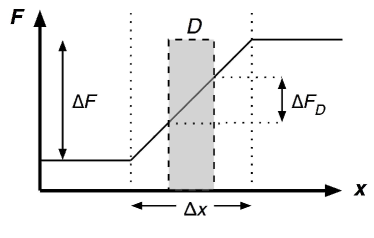
Figure 1: Sketch showing the variation in Faraday depth $F$ with respect to transverse distance in the sky plane $x$. The Faraday depth changes by $\Delta F$ across the distance $\Delta x$ and by $\Delta F_{D}$ within the beamwidth $D$.

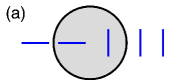
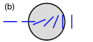
Figure 2: An illustration of depolarization in a Faraday screen: the shaded circle indicates the telescope beam, and dashes show the orientation of the polarization plane at various positions. (a) Abrupt change of the polarization angle $\Psi$ by $90\degr$ in the middle of the telescope beam leads to complete cancellation of polarization. This can be caused by a discontinuous change in $F$ by $90\degr$ in a Faraday screen. (b) A similar but continuous change of $\Psi$ does not result in strong depolarization. (c) A continuous change in $\Psi$ by $180\degr$ can produce a canal.

Consider polarized emission from a uniform background source passing through a Faraday screen – a layer where no further emission occurs, but which rotates the polarized plane. If $F$ varies with $\mn@boldsymbol{r}_{\perp}$, adjacent lines of sight within the beam are subject to different amounts of Faraday rotation and the observed degree of polarization decreases. If the variation of $F$ within the beam, $\Delta F_{D}$ (Fig. 1), produces a $90\degr$ difference in $\Psi$, one might expect that the depolarization will be complete as illustrated in Fig. 2(a), and a canal will be observed along contours defined by $\Delta F_{D}=(n+1/2)\pi$ with $n=0,1,2,\dots$.

The situation is more subtle, though. Figure 2(b) shows $\Psi$ changing smoothly by $90\degr$ across a beam, as a result of a monotonic change in Faraday depth by the same amount, $\Delta F_{D}=\pi/2$, as in panel (a). It is obvious that polarized emission does not cancel within the beam; the polarized intensity will be lower than for a uniform arrangement of angles but there will still be a polarized signal detected with a polarization angle of about $-45\degr$.

Thus, gradients in $F$ across the beam can produce complete depolarization in a Faraday screen if $F$ changes by $\Delta F_{D}\simeq(n+1/2)\,\pi$ within a small fraction of the beam width. As shown in Fig. 3 (solid line), obtained using Eqs (2) and (4), the depth of a canal will only be less than $10\%$ of the surrounding polarized emission if the gradient in $F$ occurs over one fifth or less of the beam: $\Delta x/D\lesssim 0.2$, where $\Delta x$ is the extent of the region where the gradient occurs and $D$ is the beamwidth. Haverkorn et al. (2004) reached a similar conclusion in an analysis of the depth and profile of canals observed at $\lambda 84\,\mathrm{cm}$ (see their Sect. 4.4).

As illustrated in Figs. 2(c) and 3 (dotted line), a variation in $F$ of a magnitude $\Delta F_{D}=\pi$ across the FWHM of the Gaussian beam (i.e. $\Delta F=\pi$ and $\Delta x/D\simeq 1$) can also produce strong depolarization but now the change in polarization angle across the beam is $\Delta\Psi\simeq 0\degr$. Similarly other gradients in $F$ can significantly reduce the degree of polarization; for example $\Delta F=0.7\pi$ (dashed line in Fig. 3) across a region that is about $0.7\times$ the beamwidth will produce complete depolarization and a change in angle of $54\degr$ across the beam.

Larger gradients in $F$ also result in strong depolarization and when $\Delta F>\pi$ the degree of depolarization is less sensitive to the resolution. This is illustrated in Fig. 3 for the case where $\Delta F=1.5\pi$ (dash-dotted line); complete depolarization occurs when $\Delta x/D=0,\,1.5$ but in the range $0<\Delta x/D\lesssim 2$ the degree of polarization remains below the $10\%$ level. Thus an increment of $\Delta F=1.5\pi$, and more generally $\Delta F=(n+1/2)\pi$, will produce one beam wide canals when the gradient occurs in a region roughly equal to or less than the beamwidth, i.e. where $\Delta x/D\lesssim 1$. Other large gradients in $F$, such as $\Delta F=n\pi$, depolarize to around $10\%$ of the background $p$ and therefore can also produce canals; however in this case one beam wide canals will only be formed when $\Delta x/D\simeq 1$.

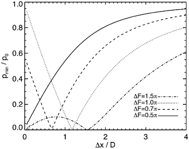
Figure 3: The minimum degree of polarization in a canal produced by a gradient of Faraday depth in a foreground screen, $p_{\mathrm{min}}$, as a function of the relative linear extent of the gradient $\Delta x/D$, where $D$ is the FWHM of a Gaussian beam and $x$ is the position in the sky-plane (see Fig. 1). Different curves represent different increments in Faraday depth, $\Delta F$ (identified in the legend). For $\Delta x/D<1$ (an unresolved gradient), $F$ changes over a distance smaller than the beamwidth and $\Delta F$ is effectively discontinuous for $\Delta x/D\ll 1$.

So, if $F$ is a continuous, random, function of position (with sufficiently strong fluctuations on the scale of the beam) we predict the existence of canals with every change in polarization angle $0\degr<\Delta\Psi<90\degr$ across the beam. On the other hand a discontinuous change in $F$ by $(n+1/2)\pi$, will produce canals across which the polarization angle changes by $\Delta\Psi=90\degr$. This insight is important as to-date all observed canals have $\Delta\Psi\simeq 90\degr$. The only other way in which Faraday screens can consistently produce canals with this change in angle is if all the gradients in Faraday depth on the approximate scale of the beamwidth are of the magnitude $\Delta F\simeq(n+1/2)\pi$, $n=1,2,\dots$ ($n=0$ in this case only produces weak depolarization, as noted above); this is extremely unlikely in a random medium.

If a system of observed canals has $\Delta\Psi=90\degr$ and is caused by a foreground Faraday screen — see Section 4 for a diagnostic test for the origin of canals — then the distribution of rotation measure in the screen must be discontinuous on the scale of the beam. Haverkorn & Heitsch (2004) used MHD simulations of Mach $10$ turbulence to show that $\mathrm{RM}$ gradients can be steep enough to produce depolarized canals on smoothing with a sufficiently large simulated beam. Note that a finite beam size is essential for the production of canals by this mechanism; with perfect resolution the width of the shock front will be resolved and no canal will appear. Furthermore, these canals will not fill up if the data are smoothed (solid and dash-dotted curves for $\Delta x/D\rightarrow 0$ in Fig. 3) whereas canals produced by gradients other than $\Delta F=(n+1/2)\pi$ will disappear under smoothing at a rate shown with dashed and dotted curves in Fig. 3.

2.1 The mean separation of canals produced by shocks

An obvious source of Faraday depth discontinuities are shocks in the ISM. Then the mean distance between the canals produced by a Faraday screen will be related to the distance between the shock fronts. The expected separation of suitable shock fronts can be derived using the model of interstellar shock-wave turbulence of Bykov & Toptygin (1987) and then compared with the separation of canals observed by Haverkorn, Katgert & de Bruyn (2003), claimed to arise in a Faraday screen.

If the frequency distribution of interstellar shocks of Mach number $\mathcal{M}$ is $\mathcal{G}(\mathcal{M})$, the mean number of shocks of a strength exceeding $\mathcal{M}$ that cross a given position in the ISM per unit time can be obtained as

$$N(\mathcal{M})=\int_{\mathcal{M}}^{\infty}\mathcal{G}(\mathcal{M})\,\mathrm{d}\mathcal{M}\;,$$ (5)

and the mean separation between the shocks in three dimensions follows as

$$L(\mathcal{M})\simeq\frac{c_{s}}{N(\mathcal{M})}\;,$$ (6)

where $c_{s}$ is the sound speed. The separation in the plane of the sky is reduced by $\pi^{-1}\int^{\pi}_{0}\sin^{2}\theta\mathrm{d}\theta=1/2$ due to projection effects and multiplied by a further factor $L/d$ if the shocks occur in a region of depth $d$. At an average distance to the shocks of $d/2$, the average angular separation in the sky plane is then

$$\mathcal{L}\simeq\frac{L^{2}}{d^{2}}.$$ (7)

For supernova-driven shocks, Bykov & Toptygin (1987) derived

$$\mathcal{G}(\mathcal{M})=G_{0}[\mathcal{M}^{-(\alpha+1)}+3C(\alpha)f_{\mathrm{cl}}(\mathcal{M}-1)^{-4}]$$ (8)

allowing for both primary and secondary shocks, where $\alpha$ is a numerical factor ($\alpha=2$ for a supernova remnant in the Sedov phase, and $\alpha=4.5$ for a three-phase ISM); $C(\alpha)\approx 2.3\times 10^{-2}$, $4.1\times 10^{-3}$ for $\alpha=2$, $4.5$ respectively; $f_{\mathrm{cl}}$ is the volume filling factor of diffuse clouds that reflect the primary shocks to produce the secondary ones; $G_{0}=\alpha S\frac{4}{3}\pi r_{0}^{3}$ with $S$ the supernova rate per unit volume and $r_{0}$ the maximum radius of a primary shock. We then obtain the following expression for the separation of shock fronts with $\mathcal{M}\geq\mathcal{M}_{*}$ in three dimensions:

$$L(\mathcal{M}) \simeq 9\,\mathrm{pc}\left(\frac{c_{s}}{10\,\mathrm{km\,s^{-1}}}\right)\left(\frac{\nu_{\mathrm{SN}}}{0.02\,\mathrm{yr}^{-1}}\right)^{-1}$$ (9)

$$\mbox{}\times\left(\frac{R}{15\,\mathrm{kpc}}\right)^{2}\left(\frac{h}{50\,\mathrm{pc}}\right)\left(\frac{r_{0}}{100\,\mathrm{pc}}\right)^{-3}$$

$$\mbox{}\times\left[\frac{1}{\mathcal{M}_{*}^{\alpha}}+\frac{\alpha C(\alpha)f_{\mathrm{cl}}}{(\mathcal{M}_{*}-1)^{3}}\right]^{-1},$$

where $\nu_{\mathrm{SN}}$ is the supernovae rate and $R$ and $h$ are the radius and scale height of the star-forming disc. The term in square brackets is approximately $1$ for $\alpha=4.5$ and $\mathcal{M}_{*}=1.2$.

If the magnetic field is frozen into the gas and the gas density increases by a factor $\epsilon_{\rho}$ at the shock then so will the field strength (we neglect a factor $\sim 1/\sqrt{2}$ due to the relative alignment of the shock and field). A canal forms where $F$ increases discontinuously by $\Delta F_{D}=(n+1/2)\pi$. So the required density compression ratio is

$$\epsilon_{\rho}\simeq\sqrt{\left|\frac{\Delta F_{D}}{\langle{F}\rangle}\right|+1},$$ (10)

where $\langle{F}\rangle$ is the mean value of $F$. The gas compression ratio depends on the shock Mach number $\mathcal{M}$ as (e.g., Landau & Lifshitz, 1960)

$$\epsilon_{\rho}=\frac{(\gamma+1)\mathcal{M}^{2}}{(\gamma-1)\mathcal{M}^{2}+2}\simeq 4\frac{\mathcal{M}^{2}}{\mathcal{M}^{2}+3}\;,$$ (11)

where we have used $\gamma\simeq 5/3$ for the ratio of specific heats, which yields the value of the shock Mach number required to produce a canal:

$$\mathcal{M}_{*} \simeq \left(\frac{3\epsilon_{\rho}}{4-\epsilon_{\rho}}\right)^{1/2}$$ (12)

$$= \left(\frac{4}{3(|\Delta F_{D}/\langle{F}\rangle|+1)^{1/2}}-\frac{1}{3}\right)^{-1/2}.$$

In the field of canals observed by Haverkorn et al. (2003) at $\lambda 84\,\mathrm{cm}$, $\langle{\mathrm{RM}}\rangle\simeq-3.4\,\mathrm{rad}\,\mathrm{m}^{-2}$ and a by-eye estimate of their mean separation gives $\mathcal{L}\simeq 45^{\prime}$. The most abundant canals are produced by the shocks which can generate $\Delta F_{D}=\pi/2$ and from Eq. (12) this requires $\mathcal{M}_{*}\simeq 1.2$. Using $f_{\mathrm{cl}}=0.25$, taking $\alpha=4.5$ and the parameter values used to normalize Eq. (9), we obtain $L\simeq 10\,\mathrm{pc}$ for shocks with $\mathcal{M}\geq\mathcal{M}_{*}$. Our estimate of $L$ includes shocks with $\mathcal{M}>\mathcal{M}_{*}$ that will not produce canals, but the strong dependence of $\mathcal{G}$ in Eq. (8) on Mach number means that $L$ will underestimate the separation of canal generating shocks insignificantly. Using Eq. (7), with $L\simeq 10\,\mathrm{pc}$ and $\mathcal{L}\simeq 45^{\prime}$, we find that the canals observed by Haverkorn et al. (2003) are compatible with a system of shocks occurring in a Faraday screen with a depth of $d\simeq 100\,\mathrm{pc}$. The maximum distance in this field, beyond which emission is completely depolarized, is estimated to be $\sim 600\,\mathrm{pc}$ by Haverkorn et al. (2003). Thus this model for the canals’ origin requires that the nearest $100\,\mathrm{pc}$ in the direction $(l,b)=(161\degr,\,16\degr)$ is effectively devoid of cosmic ray electrons; if the cosmic rays normally spread over a distance $v_{\mathrm{A}}t\sim 1\,\mathrm{kpc}$, where $v_{\mathrm{A}}\simeq 20\,\mathrm{km\,s^{-1}}$ is the Alfvén speed and $t\simeq 3\times 10^{7}\,\mathrm{yr}$ their lifetime, such a condition is difficult to explain.

3 Canals produced by differential Faraday rotation

In Section 2 we discussed the depolarization effects of Faraday rotation measure gradients transverse to the line of sight acting on smooth polarized background emission. Now we will consider a uniform layer in which both emission and Faraday rotation occur. This gives rise to the well known effect of differential Faraday rotation (Burn, 1966; Sokoloff et al., 1998), where polarized emission from two positions along the line of sight separated by a rotation of $\Delta\phi=\pi/2$ exactly cancel, thus reducing the degree of polarization. When a line of sight has a total rotation of $F=n\pi$ there is total cancellation of all polarized emission in the layer and the degree of polarization is $p=0$. Canals produced by this mechanism are discussed by Shukurov & Berkhuijsen (2003).

3.1 Differential Faraday rotation in a non-uniform medium

We now investigate how canals produced by differential Faraday rotation are affected by deviations from uniformity in the magneto-ionic medium. First we will discuss the case of a two-layer medium in which the synchrotron emissivity is different in each layer. Then we allow for random fluctuations of $F$ (the latter case produces what is known as Faraday dispersion).

For a two-layer medium the fractional polarization can be written as

$$p^{2} = \frac{p_{0}^{2}}{I^{2}}\left(I_{\mathrm{1}}^{2}\frac{\sin^{2}F_{\mathrm{1}}}{F_{\mathrm{1}}^{2}}+I_{\mathrm{2}}^{2}\frac{\sin^{2}F_{\mathrm{2}}}{F_{\mathrm{2}}^{2}}\right.$$ (13)

$$\left.+2I_{\mathrm{1}}I_{\mathrm{2}}\frac{\sin F_{\mathrm{1}}\sin F_{\mathrm{2}}}{F_{\mathrm{1}}F_{\mathrm{2}}}\cos F\right)$$

where we have assumed $\psi_{0}=0$, $I_{\mathrm{1}}$ and $I_{\mathrm{2}}$ are the synchrotron fluxes from the furthest and nearest layers to the observer respectively, $I=I_{\mathrm{1}}+I_{\mathrm{2}}$, and $F_{\mathrm{1}}$ and $F_{\mathrm{2}}$ are the Faraday depths through the two layers. [This is similar to Eq. (10) in Sokoloff et al. (1998), but with typos corrected.] We assume that $F=F_{\mathrm{1}}+F_{\mathrm{2}}=\pi$, the condition for canals to form due to differential Faraday rotation, and investigate what will happen to the canals if $I_{\mathrm{1}}\neq I_{\mathrm{2}}$. We parametrize the difference in the synchrotron emissivity in the two layers as $\epsilon=(I_{\mathrm{2}}-I_{\mathrm{1}})/I_{\mathrm{1}}$, choose equal Faraday rotation through each layer for simplicity so $F_{\mathrm{1}}=F_{\mathrm{2}}=\pi/2$, and substitute these into Eq. (13). We then obtain the dependence of the minimum degree of polarization on $\epsilon$:

$$\frac{p}{p_{0}}=\frac{|\epsilon|}{\pi}\frac{1}{(1+\epsilon/2)^{2}}\simeq\frac{|\epsilon|}{\pi}-\mathcal{O}(\epsilon^{2}).$$ (14)

Thus, for a moderate difference in emissivity of $\epsilon=1/2$ between two layers the canals will have a depth of $p/p_{0}\simeq 1/6$ compared to $p/p_{0}=0$ for a strictly uniform medium; these canals will still be clearly visible and can be interpreted as e.g. contours of $F$ or $\mathrm{RM}$ (Shukurov & Berkhuijsen, 2003). Where the difference in emissivity is greater, say $\epsilon\sim 2$ or more as one might expect viewing distant bright spiral arm emission near the Galactic plane, the canals will more readily fill up, become much less distinct and more difficult to interpret confidently.

Now let us consider the effect of random fluctuations in Faraday rotation, sometimes called internal Faraday dispersion. We start with Eq. (34) of Sokoloff et al. (1998):

$$\mathcal{P}=p_{0}\frac{1-\exp(-S)}{S},$$ (15)

where $S=2\sigma_{F}^{2}-2iF$ and $\sigma_{F}$ is the standard deviation of the Faraday depth $F$. In order to produce canals we need $F=\pi$ and then

$$\frac{p}{p_{0}}\simeq\frac{\sigma_{F}^{2}}{\pi}\left(1-\frac{1}{2}\frac{\sigma_{F}^{4}}{\pi^{2}}\right),\hskip 14.22636pt\sigma_{F}\ll 1.$$ (16)

The term in brackets shows the powerful depolarization resulting from internal Faraday dispersion (see Sokoloff et al. (1998)): for large enough $\sigma_{F}$ depolarization is complete. However, as long as $\sigma_{F}<1$, canals produced by differential Faraday rotation will only fill up by $1/3$ or less. For example, at $\lambda 20\,\mathrm{cm}$ the canals will not be destroyed as long as the dispersion in Faraday rotation measure is less than $30\,\mathrm{rad}\,\mathrm{m}^{-2}$. This is why canals are still visible in the $\lambda 20\,\mathrm{cm}$ map studied by Shukurov & Berkhuijsen (2003) which has a dispersion in rotation measure of about $\sigma_{\mathrm{RM}}\simeq 10\,\mathrm{rad}\,\mathrm{m}^{-2}$, i.e. $\sigma_{F}=\sigma_{\mathrm{RM}}\lambda^{2}\simeq 0.4$.

4 Observational diagnostics for the origin of a canal

The complex polarization emitted by a layer producing differential Faraday rotation can be written as (Burn, 1966)

$$\mathcal{P}=p_{0}\frac{\sin F}{F}\,\mathrm{e}^{2\,\mathrm{i}(\psi_{0}+F/2)}.$$ (17)

We can see immediately that if $\psi_{0}=0$ we have $Q/I=\mathrm{Re}\,\mathcal{P}\propto\sin F\cos F$ and $U/I=\mathrm{Im}\,\mathcal{P}\propto\sin^{2}F$. Since the orientation of the coordinate system in which $Q$ and $U$ are defined is arbitrary (i.e. the reference line from which we measure polarization angles can have any orientation), we can always choose a system in which $\psi_{0}=0$ near a canal. At the axis of a canal $Q=U=0$, but in the case of a canal produced by differential Faraday rotation there exists a reference frame in the ($Q$, $U$) plane where one of the two Stokes parameters changes sign across a canal but the other does not.

If, otherwise, a canal is produced by discontinuities in Faraday rotation across the beam (Sect. 2) we have (Fletcher & Shukurov, 2006a)

$$\mathcal{P}=\frac{Q+\,\mathrm{i}U}{I}=p_{0}\frac{\sin\Delta F_{D}}{\Delta F_{D}}\,\mathrm{e}^{2\,\mathrm{i}(\psi_{0}+F)},$$ (18)

in the vicinity of a canal and both $Q$ and $U$ will change sign across a canal (given $\psi_{0}=0$) except in the special case $\Delta F_{D}=F+2n\pi$. The change in sign occurs since $Q/I=p_{0}\cos[2(\psi_{0}+F)]$ on one side of the canal and $Q/I=p_{0}\cos[2(\psi_{0}+F)+\pi]$ on the other: a similar variation occurs in $U/I$. Therefore the behaviour of the observed Stokes parameters $Q$ and $U$ across a canal provides a way to distinguish between canals produced by foreground Faraday screens and those resulting from differential Faraday rotation.

5 Summary

The main points of this paper can be summarized as follows:

1. The behaviour of the Stokes parameters $Q$ and $U$ in the vicinity of a canal allows one to identify whether a foreground Faraday screen or differential Faraday rotation is the cause of the canal (Section 4).

2. A foreground Faraday screen can produce canals with any polarization angle change across the canal, $0<\Delta\Psi<90\degr$. However, discontinuous jumps in the Faraday depth will only produce canals with $\Delta\Psi\simeq 90\degr$ (Section 2).

3. If shocks produce the discontinuities in a foreground Faraday screen that generate canals, the mean separation of the canals can provide information about the Mach number and separation of shocks in the screen (Section 2.1).

4. Canals produced by differential Faraday rotation are sensitive to non-uniformity in the medium along the line of sight, systematic or random. However, they will remain recognisable if the synchrotron emissivity varies by less than a factor of about $2$ or if the standard deviation of the Faraday depth is $\sigma_{F}<1$ (Section 3.1).

References

- Beck (1999) Beck R., 1999, in Berkhuijsen E. M. ed., Galactic Foreground Polarization. MPIfR, Bonn, p.3.
- Burn (1966) Burn B. J., 1966, MNRAS, 133, 67
- Bykov & Toptygin (1987) Bykov A. M., Toptygin, N., 1987, Ap&SS, 138, 341
- Duncan et al. (1999) Duncan A. R., Reich P., Reich W., Fürst E., 1999, A&A, 350, 447
- Eilek (1989) Eilek J. A., 1989, AJ, 98, 244
- Fletcher & Shukurov (2006a) Fletcher A., Shukurov A., 2006, in Boulanger F., Miville-Deschenes M. A. eds., Sky Polarization at Far-Infrared to Radio Wavelengths: the Galactic Screen before the Cosmic Microwave Background, EAS Publications Series, Paris, in press. (astro-ph/0602536)
- Gaensler et al. (2001) Gaensler B. M., Dickey J. M., McClure-Griffiths N. M., Green A. J., Wieringa M. H., Haynes R. F., 2001, ApJ, 549, 959
- Gray et al. (1999) Gray A. D., Landecker T. L., Dewdney P. E., Taylor A. R., Willis A. G., Normandeau M., 1999, ApJ, 514, 221
- Haverkorn et al. (2000) Haverkorn M., Katgert P., de Bruyn A. G., 2000, A&A, 356, L13
- Haverkorn & Heitsch (2004) Haverkorn M., Heitsch F., 2004, A&A, 421, 1011
- Haverkorn et al. (2003) Haverkorn M., Katgert P., de Bruyn A. G., 2003, A&A, 403, 1031
- Haverkorn et al. (2004) Haverkorn M., Katgert P., de Bruyn A. G., 2004, A&A, 427, 549
- Landau & Lifshitz (1960) Landau L. D., Lifshitz E. M., 1960, Fluid Mechanics, Pergamon Press, Oxford
- Reich (2006) Reich W., 2006, in Fabbri R., ed., Cosmic Polarization. Research Signpost, in press. (astro-ph/0603465)
- Shukurov & Berkhuijsen (2003) Shukurov A., Berkhuijsen E. M., 2003, MNRAS, 342, 496 (Erratum: 2003, MNRAS, 345, 1392)
- Sokoloff et al. (1998) Sokoloff D. D., Bykov A. A., Shukurov A., Berkhuijsen E. M., Beck R., Poezd A. D., 1998, MNRAS, 299, 189 (Erratum: 1999, MNRAS, 303, 207)
- Spangler (1982) Spangler S. R., 1982, ApJ, 261, 310
- Uyaniker et al. (1998) Uyaniker B., Fürst E., Reich W., Reich P., Wielebinski R., 1998, A&AS, 138, 31
- Wieringa et al. (1993) Wieringa M. H., de Bruyn A. G., Jansen D., Brouw W. N., Katgert P., 1993, A&A, 268, 215
- Wolleben et al. (2006) Wolleben M., Landecker T. L., Reich W., Wielebinski R., 2006, A&A, 448, 411