Disentangling the synchrotron and Inverse Compton variability in the X-ray emission of the intermediate
BL Lac object S5 0716+71

Abstract

Context. The possibility to detect simultaneously in the X-ray band the synchrotron and Inverse Compton (IC) emission of intermediate BL Lac objects offers the unique opportunity to study contemporaneously the low- and high-energy tails of the electron distribution in the jets of these sources.

Aims. We attempted to disentangle the X-ray spectral variability properties of both the low- and high-energy ends of the synchrotron and Inverse Compton emission of the intermediate BL Lac object S5 0716+71.

Methods. We carried out spectral, temporal and cross-correlation analyses of the data from a long XMM-Newton pointing of S5 0716+71 and we compared our findings with previous results from past X-ray observations.

Results. Strong variability was detected during the XMM exposure. Both the synchrotron and Inverse Compton components were found to vary on time scales of hours, implying a size of the emitting region of $R\la 0.7\delta/(1+z)$ light-hours. The synchrotron emission was discovered to become dominant during episodes of flaring activity, following a harder-when-brighter trend. Tight correlations were observed between variations in different energy bands. Upper limits on time lags between the soft and hard X-ray light curves are of the order of a few hundred seconds.

1 Introduction

BL Lac objects, as well as Flat Spectrum Radio Quasars (FSRQ), are the most extreme radio-loud Active Galactic Nuclei (AGN). One of their most striking properties is the strong and rapid variability at all wavelengths. The observed radiation from BL Lac objects is commonly believed to be dominated by non-thermal emission from a jet pointing roughly towards the observer and moving at relativistic velocity (Blandford & Rees 1978). The Spectral Energy Distributions (SED) of BL Lacs are typically characterized, in $\nu$-$\nu F_{\nu}$ representation, by two broad bumps. The low-energy one, peaking at frequencies from the IR up to the soft X-ray band, is usually interpreted as synchrotron emission by a population of relativistic electrons in the jet. The high-energy one, peaking at gamma-ray energies, is supposed to be Inverse Compton (IC) radiation by the same population of electrons, scattering either the synchrotron photons themselves (Synchrotron Self-Compton, SSC; e.g. Jones, O’Dell & Stein 1974; Maraschi et al. 1992; Kirk & Mastichiadis 1997) or external photons from the surrounding environment (External Compton, EC; e.g. Dermer et al. 1992; Sikora et al. 1994).
BL Lac objects were originally divided into radio-selected (RBL) and X-ray-selected (XBL), according to the waveband of their discovery (Ledden & O’Dell 1985). A more physical classification (Padovani & Giommi 1995) separates BL Lacs depending on whether the synchrotron peak is situated at IR-optical frequencies (Low-energy-peaked BL Lacs, LBL) or in the UV/soft X-ray band (High-energy-peaked BL Lacs, HBL).
HBL are the brightest BL Lacs in the X-ray band and thus they are the best studied ones at these energies. The soft ($\Gamma\ga 2$) and continuously steepening towards higher energies X-ray spectra of HBL (Perlman et al. 2005) are commonly interpreted in terms of synchrotron radiation from the high-energy tail of the electron distribution. This tail is expected to be very sensitive to particle acceleration and cooling time scales and thus to be mostly affected by rapid and strong variability (Kirk & Mastichiadis 1997). X-ray observations of the closest and X-ray brightest HBL (PKS 2155-305: e.g. Chiappetti et al. 1999; Edelson et al. 2001; Zhang et al. 2005; MRK 421: e.g. Takahashi et al. 1996; Fossati et al. 2000; Brinkmann et al. 2005; MRK 501: e.g. Pian et al. 1998; Tavecchio et al. 2001), have indeed revealed strong variability, characterized by large amplitude variations, both on long and short time scales (fastest flux changes of $\sim 2$ on time scales of the order of a few hours; Sembay et al. 1993; Zhang et al. 2002). The variability amplitude has been found to be correlated with energy (Sembay et al. 2002; Zhang et al. 2005; Gliozzi et al. 2006), in agreement with the hypothesis that the hardest synchrotron radiation is produced by the most energetic electrons with the smallest cooling time scales. Flux increases are typically accompanied by spectral hardening, with the remarkable exception of the July 1997 flare of MRK 501, which exhibited an opposite behaviour (Lamer & Wagner 1998). However, from a recent reanalysis of the 1997 RXTE data, Gliozzi et al. (2006) concluded that this was a spurious result. Shifts of the synchrotron peaks, up to two orders of magnitude in the case of MRK 501, towards higher energies have been observed during extreme flaring activity (Pian et al. 1998; Giommi et al. 2000; Tavecchio et al. 2001). Light curves in different X-ray bands have been found to be well correlated, often with delays of the order of a few hours. However, independent variability in different X-ray bands has also been observed during the RXTE observations of MRK 501 in July 1997 (Lamer & Wagner 1998). The length of the lags, when detected, appears to change from flare to flare. Variations at softer energies usually lag behind those at harder energies (soft lags), although the opposite behavior (hard lags) has also been claimed (PKS 2155-305: Zhang et al. 2006; MRK 421: Fossati et al. 2000). Time lags lead to spectral changes with flux characterized, in spectral index vs. intensity ($\alpha-I$) plots, by clockwise (soft lags) or counter-clockwise (hard lags) loop patterns, effectively observed in some cases (e.g. Takahashi et al. 1996; Zhang et al. 2002; Ravasio et al. 2004; Brinkmann et al. 2005). The sign of the time lags and the paths traced in the $\alpha-I$ plane have been directly related to differences in the acceleration and cooling time scales of the system for the energy bands considered (Kirk, Rieger & Mastichiadis 1998). This in turn has been used to impose constraints on some of the physical parameters of the emitting regions, such as the magnetic field and the Lorentz factors of the particles.
On the other hand, the X-ray emission of LBL is believed to originate mainly from IC scattering of seed photons by the low-energy tail of the electron population, although the synchrotron emission of the high-energy particles might still contribute significantly. For a few objects with synchrotron peaks located around $10^{14}-10^{15}$ Hz, known as intermediate BL Lac objects (IBL), the X-ray observations have clearly detected the turning point of their SED, where the synchrotron and IC components intersect (ON 231: Tagliaferri et al. 2000; BL Lacertae: Tanihata et al. 2000; Ravasio et al. 2002; S5 0716+71: Cappi et al. 1994; Wagner et al. 1996; Giommi et al. 1999; Tagliaferri et al. 2003; AO 0235+16: Raiteri et al. 2006; OQ 530: Tagliaferri et al. 2003). X-ray studies of both flux and spectral variability of LBL/IBL are thus able, in principle, to convey information on the physical conditions of both the low- and high-energy electrons simultaneously; in the case of HBL this goal can be achieved only through contemporaneous multi-frequency observations. However, due to their lower X-ray luminosities as compared with HBL, only a few X-ray studies of LBL/IBL have been carried out so far. In general, the X-ray variability of known LBL/IBL shows similar characteristics as HBL, both in terms of amplitude and time scales. However, contrary to HBL, the variability amplitude seems to decrease at harder energies (Giommi et al. 1999; Ravasio et al. 2002), where the IC component becomes dominant. This finds a natural explanation in the longest cooling time scales of the lowest energy electrons responsible for the IC emission. Short time scale ( $\la$ hours) variability seems to be present only in the synchrotron component, whereas the IC emission appears to vary on longer time scales ($\sim$ days). To our knowledge, no time lags between different X-ray bands or loops in the $\alpha-I$ plane have been reported so far for LBL/IBL, although they might be expected (Böttcher & Chiang 2002).
In this paper we present the analysis of an archival XMM-Newton observation of S5 0716+71, lasting $\sim 59$ ks. It is the longest uninterrupted, highest signal-to-noise ratio X-ray observation performed so far for this source, thus providing the possibility to disentangle with great accuracy the relative contributions, within the XMM band, of the synchrotron and IC components, and to determine the variability properties of both of them.
Recently, a separate study of the same XMM data set was presented by Foschini et al. (2006) during the submission process of our manuscript. Their results are briefly compared with ours in Sect. 8.
The outline of the paper is the following: in Sect. 2 we give more details on the source and we summarize briefly the results from past X-ray observations; in Sect. 3 we describe the data processing; in Sects. 4 and 5 we give, respectively, the results of the spectral and timing analysis; in Sect. 6 we analyze the spectral variability of the source; in Sect. 7 we examine the Optical Monitor data; in Sect. 8 we summarize and discuss the results, and in Sect. 9 we give our conclusions.

2 Past X-ray observations

S5 0716+71 is one of the brightest and most active BL Lac objects in the sky. It was initially discovered in the 5 GHz Bonn-NRAO radio survey and was included in the S5 catalog of strong ($S>1$ Jy), flat ($\alpha\leq 0.5$, $S\propto\nu^{-\alpha}$) radio sources with declination $\delta\geq 70^{\circ}$ (Kühr et al. 1981). In spite of its optical brightness ($m_{\rm V}\sim 13.0$), its spectrum does not show any emission or absorption feature which, together with its high linear polarization, led to its classification as a BL Lac object (Biermann et al. 1981). An upper limit on the redshift of $z>0.3$ was estimated from the lack of any detection of the host galaxy in optical images (Wagner et al. 1996). Recently, Sbarufatti et al. (2005) proposed a new lower limit of $z>0.52$ using HST images. S5 0716+71 is a well known intra-day variable (IDV) source with a very high variability duty cycle and it has been intensively studied at all frequencies since its discovery. In particular, S5 0716+71 has been the target of a number of multi-frequency campaigns (e.g. Wagner et al. 1990; Quirrenbach et al. 1991; Wagner et al. 1996; Ostorero et al. 2006). The synchrotron peak of its SED falls around $10^{14}$ Hz (Wagner & Witzel 1995; Ostorero et al. 2006).
S5 0716+71 has also been observed several times by various X-ray telescopes and some of the results are summarized in Table 1. Biermann et al. (1992) were the first to report an X-ray flux from a HEAO-A observation in 1977. The source was then observed by the Einstein satellite in 1979 and 1980; however, the counts were too low to determine a spectrum and only a flux estimate could be given (Biermann et al. 1981). A spectral and temporal analysis was possible for the first time with ROSAT, which observed S5 0716+71 with the PSPC in March 1991 (Wagner 1992; Cappi et al. 1994; Urry et al. 1996; Wagner et al. 1996). These observations suggested that two distinct spectral components are necessary to account for the X-ray spectrum in the 0.1–2.4 keV band and these components were interpreted as synchrotron and IC emission, respectively. The same data clearly revealed for the first time in this source flux variability with associated spectral variations. In 1994, S5 0716+71 was observed by ASCA as part of a series of multi-wavelength campaigns on a sample of blazars (Kubo et al. 1998). ASCA confirmed the existence of a spectral flattening with increasing energies, in agreement with the ROSAT results. During a multi-frequency campaign in 1996, S5 0716+71 was the target of simultaneous ROSAT-HRI (0.1–2.4 keV) and RXTE (2–10 keV) pointings. No correlation could be established between the corresponding light curves, a result which, given the different energy range of the two instruments, pointed at the presence of a soft and hard components with different variability properties (Otterbein et al. 1998). Finally, S5 0716+71 was observed by BeppoSAX in 1996, 1998 (Giommi et al. 1999) and 2000 (Tagliaferri et al. 2000). In 1996 and 1998 the source was found in a faint state and the spectral modeling required two components, similarly to previous X-ray observations. Short-term variability of the soft component below $\sim 3$ keV was detected; the hard component above $\sim 5$ keV appeared to be more stable, although some long-term variability seemed to be present from the comparison between the 1996 and 1998 data. In 2000 the source was caught in its highest state and the soft slope was the largest of the three BeppoSAX observations, suggesting a softer-when-brighter trend, opposite to that usually observed for BL Lacs. The 2000 data confirmed the essential absence of variability above $\sim 3$ keV.

Table 1: Results from past X-ray observations (see Sect. 2 for further details).

Date	Instrument	$\Gamma_{\rm soft}$	$E_{\rm break}$ (keV)	$\Gamma_{\rm hard}$	Band (keV)	$F$ (erg cm-2 s-1)	$F_{\rm 1\leavevmode\nobreak\ keV}$ (erg cm-2 s-1Hz-1)	Ref.
2 Oct 1977	HEAO-A	(1.5)∗			0.25–25		$1.28\times 10^{-29}$	(2)
29 Aug 1979	Einstein	(1.5)∗			0.2–3.5	$2.89\times 10^{-12}$	$0.41\times 10^{-29}$	(1)
19 Oct 1979, 9 Mar 1980	Einstein	(1.5)∗			0.2–3.5		$0.31\times 10^{-29}$	(2)
8/11 Mar 1991 (low state)	ROSAT-PSPC	$3.99^{\rm+4.21}_{\rm-3.81}$		$2.25^{\rm+2.65}_{\rm-1.25}$	0.1–2.4	$3.73\times 10^{-11}$	$1.03\times 10^{-29}$	(3)
8/11 Mar 1991 (high state)	ROSAT-PSPC	(3.99)∗		(2.25)∗	0.1–2.4	$8.45\times 10^{-11}$	$2.98\times 10^{-29}$	(3)
16/19/21 Mar 1994	ASCA				2–10	$1.30\times 10^{-12}$		(4)
24 Mar–22 Apr 1996	ROSAT-HRI							(5)
6–22 Apr 1996	RXTE			3.1$\pm$0.1	2–10			(5)
14 Nov 1996	BeppoSAX	2.7$\pm$0.3	2.3$\pm$0.4	1.96$\pm$0.15	2–10	$1.4\times 10^{\rm-12}$		(6)
7 Nov 1998	BeppoSAX	2.3$\pm$0.4	2.8$\pm$0.8	1.73$\pm$0.18	2–10	$2.6\times 10^{\rm-12}$		(6)
30/31 Oct 2000	BeppoSAX	$3.40^{\rm+0.4}_{\rm-0.3}$		$1.60^{\rm+0.25}_{\rm-0.35}$	2–10	$3.3\times 10^{\rm-12}$	$1.80\times 10^{-29}$	(7)

* Fixed photon index. (1) Biermann et al. (1981), (2) Biermann et al. (1992), (3) Cappi et al. (1994), (4) Kubo et al. (1998), (5) Otterbein et al. (1998), (6) Giommi et al. (1999), (7) Tagliaferri et al. (2003).

3 The XMM-Newton observation

S5 0716+71 was observed by XMM-Newton (Jansen et al. 2001) for $\sim$ 59 ks on April 4–5, 2004 (Obs. ID 0150495601, Rev. 791, PI G. Tagliaferri). The technical information about the observation is summarized in Table 2.
Calibrated and concatenated event lists were produced from the Observation Data Files (ODF) with

mmsas } v. 6.5.0, following
standard procedures  and with the most recent
calibration files available at the time of the analysis.  Due to a
bug of the {\verb omfchain } pipeline (SSC-SPR-3499)
the data from the Optical
Monitor (OM; Mason et al. 2001) were processed with {\verb 

mmsas v. 6.1.0.
Pile-up effects in the EPIC PN (Strüder et al. 2001) and EPIC MOS (Turner et al. 2001) data were checked with the task patplot } and found to b acceptable (observed-to-predicted single and double event ratios $\sim 1$). We restricted the analysis of PN data in Timing Mode to the energy range over which the observed and predicted single and double event fractions were found to agree well, i.e. between 0.5–10.0 keV. For consistency, we used the same energy range for the analysis of the MOS data, excluding as well any remaining (cross-)calibration uncertainties below $\sim 0.3$ keV (Kirsch 2006).
As the observation was affected by soft-proton flares, only Good Time Intervals (GTI) were selected for the analysis after the inspection of the background light curves of the different instruments. The resulting effective exposures are given in Table 2. One should notice that, due to the use of the thick filter, the MOS 2 camera is less sensitive to background flares and therefore the GTI selection yields a much longer effective exposure than for the PN and MOS1. The way this time selection affects the spectral analysis is discussed in Sect. 4.
We extracted source counts for the PN from a central strip with $28\leq{\rm RAWX}\leq 47$ and background counts from two strips at the sides of the CCD with $2\leq{\rm RAWX}\leq 11$ and $54\leq{\rm RAWX}\leq 63$. Source counts for MOS1 and MOS2 were extracted from circular regions centered on the source with radii of 27 and 60 arcsec, respectively, where the smaller radius for MOS1 is due to the use of the Small Window Mode. Background counts have been extracted from circles of the same size and located on the same CCD as the source regions. In the case of MOS1 in Small Window Mode care was taken to choose a background region least affected by the source counts. Only single and double events (PN) and single-to-quadruple events (MOS) with quality FLAG=0 were used in the analysis.
PN and MOS spectra were created with vslect and grouped with rppha } in order to have at least 30 counts in each enery bin for the use of the $\chi^{2}$ statistics. Redistribution matrices and ancillary response files were produced with mfgen } and {\veb arfgen , respectively.
RGS (den Herder et al. 2001) spectra and response matrices have been created with gspoc . We have considered only the 0.8-2.0 keV band, excluding lower energies where the RGS show a 30-40% flux loss with respect to the PN and MOS cameras (Stuhlinger et al. 2006).
The spectral analysis was performed with XSPEC v. 11.3.1., whereas the timing analysis was carried out with FTOOLS v. 5.3.1. and our own routines.

Three other short observations (Obs. IDs 0012850101, 0012850601, 0012850701, PI J. Mulchaey), in which S5 0716+71 was in the field of view, were found in the XMM archive. They were performed on April 13, 2001, September 19, 2001 and March 26, 2002, respectively. The target of these observations was the cluster 1WGA J0720.8+7108 at z=0.23, whereas S5 0716+71 was lying at $\sim 12$ arcmin from the boresight. The PN and MOS cameras were operated in Full Frame Mode with a thin filter, except for obs. ID 0012850601 for which no PN data were taken. However, the source counts from these three observations are much lower than that from the 2004 data, both due to the shorter exposures and to the stronger vignetting. Furthermore, sources observed at off-axis angles larger than $\sim 10$ arcmin suffer from large calibration and vignetting correction uncertainties (Kirsch 2006). For the above reasons we do not report on the detailed analysis of these data; however, for completeness, in Sect. 4 we quote the fluxes of the source at the three different epochs, using the results of the spectral analysis from the 2004 observation.
In the following, a cosmology with $H_{\rm 0}=70$ km s^-1 Mpc^-1, $\Omega_{\rm M}=0.27$ and $\Omega_{\rm\Lambda}=0.73$ is assumed.

Table 2: Summary of the XMM-Newton observation of S5 0716+71 during April 4–5, 2004.

EPIC+RGS
Instrument	Mode	Filter	Energy band (keV)	Effective exposure∗ (s)	Net count rate (cts/s)
PN	Timing	Thin	0.5-10.0	48491	4.42
MOS1	Small Window	Thin	0.5–10.0	46808	1.59
MOS2	Full Frame	Thick	0.5–10.0	54144	1.38
RGS1	Spectroscopy	-	0.8–2.0	37025	0.22 (order 1)
					0.04 (order 2)
RGS2	Spectroscopy	-	0.8–2.0	35672	0.23 (order 1)
					0.03 (order 2)
Optical Monitor
Mode	Filter	Wavelength (nm)	N. exposures	Total effective exposure (s)
Imaging+Fast	V	543	8	9600
Imaging+Fast	U	344	10	12000
Imaging+Fast	UVW1	291	5	6000
Imaging+Fast	UVM2	231	5	6000
Imaging	UVW1	291	5	4000
Imaging	UVM2	231	5	4000

* After selection of Good Time Intervals.

4 Spectral analysis

We started by carrying out the spectral analysis for the entire observation, without combining the data from different instruments. We restricted the analysis of PN and MOS data to the 0.5–10.0 keV band as explained in Sect. 3. In the spectral fits we used the Galactic neutral hydrogen column density measured towards the source by Murphy et al. (1996), corresponding to $N_{\rm H}=3.05\times 10^{20}$ cm^-2. All quoted errors are 90% confidence ($\Delta\chi^{2}=2.706$ for one interesting parameter) unless otherwise stated. The results of the spectral fits are summarized in Table 3. We remark that the detailed numerical values for the three detectors may differ, because of the use of different GTIs combined with the strong spectral variability of the source (see later on), but the physical models which describe the data should be the same.
We first attempted to fit the data with the simplest model, a power law plus Galactic absorption. The fit is clearly not acceptable, with large positive residuals above $\sim 3$ keV, indicating a flattening of the spectrum at high energies (see Fig. 1). Letting $N_{\rm H}$ free to vary does not improve the fit significantly and yields an absorption much lower than the Galactic value.
A good fit is obtained using a broken power law plus Galactic absorption (see Fig. 2). No need for extra absorption is found when $N_{\rm H}$ is left as a free parameter. From the broken power law model we obtain PN unabsorbed fluxes in the total and hard bands of $F_{\rm 0.5-10\leavevmode\nobreak\ keV}=1.01^{\rm+0.01}_{\rm-0.02}\times 10^{-11}$ erg cm^-2 s^-1and $F_{\rm 2-10\leavevmode\nobreak\ keV}=3.83^{\rm+0.12}_{\rm-0.14}\times 10^{-12}$ erg cm^-2 s^-1, respectively. These fluxes correspond to lower limits on the rest frame luminosities of $L_{\rm 0.5-10\leavevmode\nobreak\ keV}\geq 3.42{\rm\pm 0.03}\times 10^{45}$ erg s^-1and $L_{\rm 2-10\leavevmode\nobreak\ keV}\geq 1.15^{\rm+0.03}_{\rm-0.02}\times 10^{45}$ erg s^-1for $z\geq 0.3$.
A broken power law represents a good and simple parameterization of the X-ray spectrum of S5 0716+71 in the XMM band; however, other spectral models can in principle fit the data equally well (see Table 3). A double power law with Galactic absorption provides an equally good fit. Similarly, a power law plus the addition of a black body component is also an acceptable fit, whereas a power law plus a thermal bremsstrahlung component is an adequate fit for PN and MOS2 data, but can be accepted only at 1% significance level for MOS1.
We further attempted to fit the data with a logarithmic parabola of the form $E^{-\Gamma+\beta\log E}$. Although this is also a viable model, when compared with the broken power law or the double power law, it yields a worse fit.
Despite the fact that all the above-mentioned models, except for the single power law, constitute valid representations of the data, in agreement with previous X-ray studies and with the interpretation of the SED of S5 0716+71, we adopt the broken and double power laws as our favorite models. Both models can be interpreted easily (see Sect. 2), in terms of a mixed contribution of the hard energy tail of the synchrotron emission (steeper, soft component) and the rising side of the IC bump (flatter, hard component). The logarithmic parabola can also be interpreted in this way, with the difference that it represents a continuously curved spectrum instead of the combination of two straight power laws. However, we discard it, as it provides a worse fit to the data.
Conversely, a model comprising a power law and a black body component cannot be easily reconciled with any physical scenario for the source. The black body emission might be attributed to the accretion disk; however, we do not expect this component to contribute significantly in a BL Lac such as S5 0716+71, where the jet emission is dominant in all bands and basically no sign of thermal emission has ever been observed at any other wavelength. Furthermore, the temperature resulting from the fit is rather high and therefore the black body component appears to merely provide a parameterization of the high-energy part of the X-ray spectrum, without any real physical meaning.
A thermal bremsstrahlung component might originate from the host galaxy of the source or from a cluster around it, or close to it.  The PN unabsorbed 0.2–3.5 keV flux of the bremsstrahlung component is $4.92^{+0.27}_{-0.14}\times 10^{-12}$ erg cm^-2 s^-1, corresponding to a lower limit on the luminosity for $z>0.3$ of $1.87^{+0.11}_{-0.06}\times 10^{45}$ erg s^-1. This luminosity largely exceeds typical values for massive elliptical galaxies (Fabbiano 1989) and therefore, similarly to Cappi et al. (1994), we conclude that thermal emission from the host galaxy is unlikely. The cluster 1WGA J0720.8+7108 (see Sect. 3) could be able in principle to produce such a high luminosity; however, at the location of S5 0716+71, about 12 arcmin from the center of the cluster, it is implausible that thermal emission can contaminate significantly the flux from the BL Lac. From a time-resolved spectral analysis (the intervals used are those defined in Fig. 3, see Sect. 6), the 0.2–3.5 keV flux of the bremsstrahlung component resulted to vary significantly ($\Delta F\approx 44$%), arguing further against a host galaxy or cluster origin.
In conclusion, in the following discussions we will consider only the broken and double power law models and we will make the implicit association between the steeper (flatter) power law with the synchrotron (IC) component. We can thus see that, e.g. considering the PN, the synchrotron emission contributes to $\sim 65$% of the flux in the 0.5–10.0 keV band, whereas the IC constitutes a smaller, but not negligible, $\sim 35$%.

Table 3: Results of the spectral analysis for the entire XMM observation of S5 0716+71, on April 4–5, 2004. The neutral hydrogen column density ($N_{\rm H}$) has been fixed to the Galactic value in all fits.

Model	Instrument	$\Gamma_{1}$	$E_{\rm br}$ (keV)/$\beta^{*}$	$\Gamma_{2}/kT$ (keV)	$\chi^{2}_{\rm red}/{\rm dof}$	Prob.	$F_{\rm 2-10\leavevmode\nobreak\ keV}^{\dagger}$
Power law	PN	2.73$\pm$0.01	-	-	1.38/1451	9.30$\times 10^{-21}$	2.47${}^{+0.04}_{-0.05}$
	MOS1	2.53$\pm$0.01	-	-	1.90/281	4.90$\times 10^{-18}$	3.62${}^{+0.08}_{-0.07}$
	MOS2	2.50$\pm$0.01	-	-	1.66/306	2.47$\times 10^{-12}$	3.84${}^{+0.07}_{-0.06}$
Broken power law	PN	2.83$\pm$0.01	1.91${}^{+0.10}_{-0.08}$	2.06${}^{+0.05}_{-0.06}$	0.982/1449	0.680	3.83${}^{+0.11}_{-0.10}$
	MOS1	2.64$\pm$0.02	2.34${}^{+0.25}_{-0.16}$	2.02${}^{+0.10}_{-0.07}$	1.070/279	0.200	4.43$\pm$0.13
	MOS2	2.62$\pm$0.02	2.27${}^{+0.36}_{-0.20}$	2.11${}^{+0.06}_{-0.11}$	0.957/304	0.695	4.46$\pm$0.09
Double power law	PN	3.01$\pm$0.05	-	1.22${}^{+0.15}_{-0.22}$	0.982/1449	0.686	3.95${}^{+0.45}_{-1.16}$
	MOS1	2.72${}^{+0.08}_{-0.04}$	-	0.70${}^{+0.45}_{-0.30}$	1.038/279	0.318	4.69${}^{+0.91}_{-1.39}$
	MOS2	2.74${}^{+0.10}_{-0.06}$	-	1.13${}^{+0.35}_{-0.36}$	0.919/304	0.841	4.62${}^{+0.79}_{-1.44}$
Power law + black body	PN	2.87$\pm$0.02	-	1.71${}^{+0.14}_{-0.12}$	0.978/1449	0.721	3.45${}^{+0.27}_{-0.29}$
	MOS1	2.67$\pm$0.02	-	2.41${}^{+0.56}_{-0.33}$	1.051/279	0.268	4.59${}^{+0.45}_{-0.70}$
	MOS2	2.65$\pm$0.03	-	2.05${}^{+0.29}_{-0.19}$	0.922/304	0.830	4.45${}^{+0.31}_{-0.44}$
Power law + bremss.	PN	2.12${}^{+0.04}_{-0.06}$	-	0.31${}^{+0.02}_{-0.01}$	1.018/1449	0.307	3.75${}^{+0.09}_{-0.10}$
	MOS1	2.11$\pm$0.07	-	0.38$\pm$0.03	1.201/279	0.012	4.37${}^{+0.15}_{-0.22}$
	MOS2	2.17${}^{+0.05}_{-0.07}$	-	0.37${}^{+0.04}_{-0.03}$	1.014/304	0.422	4.44${}^{+0.14}_{-0.16}$
Logarithmic parabola	PN	2.79$\pm$0.01	0.57$\pm$0.03	-	1.008/1450	0.413	3.76${}^{+0.11}_{-0.09}$
	MOS1	2.66$\pm$0.02	0.44$\pm$0.04	-	1.108/280	0.104	4.44${}^{+0.11}_{-0.12}$
	MOS2	2.64$\pm$0.02	0.38$\pm$0.04	-	0.955/305	0.703	4.50${}^{+0.11}_{-0.10}$

* $\beta$ is the “curvature parameter” in the logarithmic parabola model (see text for the analytical formula).
$\dagger$ in units of $10^{-12}$ erg cm^-2 s^-1

Figure 1: Power law fit to the PN data (upper panel) with data-to-model ratios (bottom panel), clearly showing the upturn of the spectrum with increasing energies. Similar residuals are obtained for the MOS data.

Figure 2: Broken power law fit to the PN data (upper panel) with data-to-model ratios (second panel). Also shown are the ratios from the broken power law fits for MOS1 (third panel) and MOS2 (fourth panel).

A matter of concern are the significant discrepancies observed between the PN and MOS best fit parameters (see Table 3). In fact, it is impossible to fit the PN and MOS data jointly (e.g. a broken power law yields $\chi^{2}_{\rm red}/{\rm dof}=1.110/2038$, prob.=$3.37\times 10^{-4}$). Only when the parameters for the three cameras are left free to vary independently, except for the break energy, the fit becomes acceptable ($\chi^{2}/{\rm dof}=0.998/2034$, prob.=0.516). However, the photon indices still differ by $\Delta\Gamma\sim 0.2$ and the fluxes by $\sim$15–16%. Although PN/MOS differences are widely known, the flux discrepancies that we observe appear to be larger than what is reported in the XMM documentation (Stuhlinger et al. 2006). On the other hand, to our knowledge, investigations on PN/MOS cross-calibration uncertainties have so far not taken into account the Timing Mode, and thus we cannot compare directly our results with previous studies.
We checked whether the spectral variability of S5 0716+71, combined with the different pattern of GTI selection for the three instruments (see Sect. 3), could explain (at least part of) the observed disagreement (an extensive discussion of the spectral variability of S5 0716+71 will be given in Sect. 6). To this purpose, we extracted data from a time interval, common to PN and MOS, characterized by similar GTIs created by the standard processing pipeline, which include periods of normal functioning of the instruments. The initial $\sim 19$ ks of the observation fulfilled this criterion and were selected for the following analysis. We then applied the user-defined GTIs, based on the background light curve of the PN camera, also to MOS1 and MOS2 (we notice that no case exists in which a background flare is registered by MOS1 or MOS2 but not by the PN; therefore we do not risk to include periods of high background in the MOS data). In this way we are sure to sample similar time intervals for the three cameras, with effective exposures differing by no more than $\sim 500$ s. A joint broken power law fit to the PN and MOS spectra extracted from the above time interval was found to be acceptable ($\Gamma_{\rm 1}=2.85\pm 0.02$, $E_{\rm break}=1.81^{\rm+0.11}_{\rm-0.10}$ keV, $\Gamma_{\rm 2}=2.17\pm 0.05$, $\chi^{2}_{\rm red}/{\rm dof}=0.908/631$, prob.=0.953), contrary to the case of the whole observation. The flux differences are significantly diminished to $\sim 7-10$%, a value closer to, although still higher than those normally reported for the Imaging modes (Stuhlinger et al. 2006). We conclude that the spectral variability of the source gives a considerable contribution to the discrepancies between PN and MOS, although it cannot account entirely for it. Further investigations of the remaining discrepancies are beyond the scope of this paper; however, we remark that the errors on all the quoted fluxes do not include the $\sim 7-10$% uncertainty.

Using the PN and MOS data (separately) for the whole observation, we further estimated an upper limit on any possible intrinsic absorption in the source. To this purpose, we used the best fit broken power law model with the addition of a second redshifted component (model

wabs } in
{\verb xspec }) to the Galactic neutral
hydrogen column density. We tried
a range of values for the redshift and found that, up to 

=2, values of $N_{\rm H,int}\ga 2\times 10^{20}$ cm^-2 are not compatible with the data.

Given the importance that any detection of a line would have for the determination of the redshift of S5 0716+71, we looked in more detail for emission and absorption features in the EPIC spectra. By using the broken power law as the base model, we added to it a Gaussian emission or absorption line. We stepped the initial value of the line energy over the entire spectrum through a grid of 0.5 keV bin size and we attempted a fit for each grid point, either with both the energy and the width of the line $\sigma$ left free to vary, or with $\sigma$ fixed to 0.01 keV (i.e. a narrow line, below the energy resolution of the instruments). If the fit did not converge to any line energy, the latter was fixed to the grid point and an upper limit to either the equivalent width (EW) or to the optical depth was determined. With this procedure no line was found to be statistically significant: the fits did not improve after the addition of a line at any energy within the 0.5–10.0 keV band and no line is detected at the same energy in the spectra of the three cameras. In all cases the minimum EWs and optical depths compatible with the data are equal to zero. Upper limits on EWs for energies up to $\sim 5.8$ keV (corresponding to a neutral Fe K$\alpha$ line at $z\geq 0.1$) are of the order of $\sim 100$ eV. We also examined the RGS data, but no line could be found. As the RGS did not provide better or additional information with respect to the PN and MOS data, we do not consider them further.

Finally, we estimated the flux for the three observations in 2001–2002 by fitting a broken power law with all the parameters fixed to the 2004 best fit values for each instrument (see Table 3). Only the normalizations were left free to vary. The fits were acceptable for the 2001 observations and thus we have no reason to believe that the spectrum of the source was significantly different at that time. The comparison of the 0.5–10.0 keV MOS1 (the PN was off during the September exposure) unabsorbed fluxes of the 2001 observations ($6.68^{+0.85}_{-0.45}\times 10^{-12}$ erg cm^-2 s^-1and $9.13^{+0.80}_{-0.62}\times 10^{-12}$ erg cm^-2 s^-1) with that in 2004 ($F_{\rm 0.5-10.0\leavevmode\nobreak\ keV}=1.13\pm 0.01\times 10^{-11}$ erg cm^-2 s^-1) shows that the source was about a factor of two fainter in the earlier epoch, but with a similar flux level in the second epoch. On the other hand, a broken power law fit to the PN spectrum of the 2002 observation is acceptable only at 1% significance level and it fails when applied to the MOS data. This might be an indication that significant spectral variability took place between 2002 and 2004. However, the MOS flux in 2002, which appears to be rather insensitive to the parameter values, is about three times larger than the PN flux, casting doubts on the reliability of these data. The PN flux ($F_{\rm 0.5-10.0\leavevmode\nobreak\ keV}=8.55^{+0.35}_{-0.38}\times 10^{-12}$ erg cm^-2 s^-1) is more in line with the values that have been observed so far for S5 0716+71.

5 Temporal analysis

As a first step, we produced the 0.5–10.0 keV band background-subtracted source light curves for the three EPIC cameras separately, with a time bin size of 500 s. Photons were extracted from a time interval common to all the instruments, as the three cameras start to register events at slightly different times. The resulting effective exposures for the timing analysis are $\sim$55 ks. According to a Kolmogorov-Smirnov test, the ratios of the light curves from any pairs of instruments resulted to be consistent with being constant at 5% significance level. The light curves obtained from the three cameras, with different operating modes, filters and backgrounds, are thus consistent with each other and are not affected by periods of high background, especially important towards the end of the observation. Therefore, we summed the PN and MOS light curves up to increase the number statistics in each bin. The combined 0.5–10.0 keV light curve is shown in Fig. 3. Strong variability is clearly detected, with the shortest observed doubling time of $\sim 2.5$ ks, corresponding to the steep rise of the flux around $t\sim 5\times 10^{4}$ s. The maximum-to-minimum count rate ratio is $\ga 3$. The mean count rate is $6.59\pm 0.01$ cts/s, with an observed variance (i.e. including measurement noise) of 6.14 (cts/s)².
The beginning of the observation caught the source in a phase of decreasing flux. During the first $\sim 7-8$ ks the count rate reduced by a factor of $\sim 1/2$. The decreasing trend continued for another $\sim 10$ ks, with a slightly shallower slope and with a few small amplitude bursts. Afterwards, the count rate started to increase again, at first more slowly for $\la 8$ ks, and then resulting in a burst characterized by two or, possibly, three peaks, lasting in total $\sim 10$ ks. This high state is followed by a relatively quiescent period of $\sim 8$ ks, characterized by variations of smaller amplitude, preceding a big burst towards the end of the observation. At the beginning of this flare the count rate increased by a factor of $\sim 3$ in $\sim 4$ ks, settled itself on a flat level for $\sim 3$ ks, reached the maximum value of the entire observation in $\sim 2$ ks and decayed again. The decreasing phase of this big flare was unfortunately not fully sampled.
A measure of the intrinsic source variability is given by the fractional variability amplitude (FVA; Edelson et al. 2002; Vaughan et al. 2003). In the 0.5–10.0 keV band we found ${\rm FVA}=37\pm 2$%. The uncertainty was calculated according to the formula given in Vaughan et al. (2003) and is due to measurement errors only.

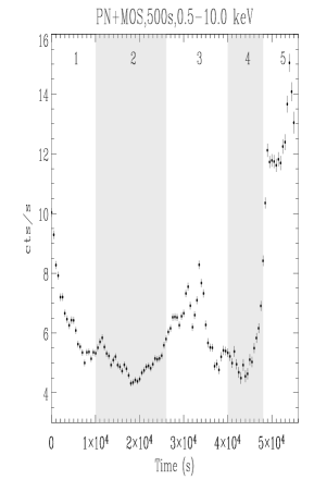
Figure 3: Combined PN+MOS light curve in the 0.5-10.0 keV band. The bin size is 500 s and the time is counted from the beginning of the observation (JD=2453099.983). The figure also shows the time intervals used for the time-resolved spectral analysis (see Sect. 6).

We checked whether and to what extent the fractional variability amplitude depended on the energy band considered. We extracted source light curves in two different energy bands: a soft one (0.5–0.75 keV) and a hard one (3.0–10.0 keV). According to the double power law spectral model (see Sect. 4), the contribution of the synchrotron (IC) component to the total flux is $\sim 89$% ($\sim 11$%) for the soft band and $\sim 29$% ($\sim 71$%) for the hard band. The soft and hard light curves, normalized to their mean count rates, are shown in Fig. 4. The variability amplitude appears more pronounced in the soft band. The FVA in the soft band ($40\pm 3$%) is indeed higher than in the hard band ($27\pm 1$%).

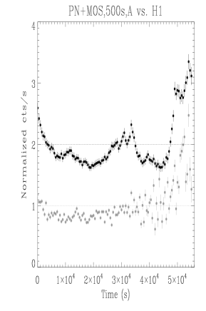
Figure 4: Combined PN+MOS light curves in the 0.5–0.75 keV (black) and 3–10 keV (gray) bands. The light curves have been normalized to their mean count rates and shifted with respect to each other for clarity. The mean level for each normalized light curve is shown with a dotted line of corresponding color. The bin size is 500 s.

In order to study the statistical characteristics of the variability of the source, we calculated the power density spectrum (PDS; Priestley 1981) of the 0.5–10.0 keV light curve between $\sim 4\times 10^{-5}$ Hz and $10^{-3}$ Hz. The result is shown in Fig. 5. The PDS does not show any precise characteristic periodicity or time scale in this time range. The PDS was re-binned according to the method of Papadakis & Lawrence (1993) and fitted with a broken power law. The break, above which the noise level is reached, was found at $\nu\sim 5\times 10^{-4}$ Hz. The fit gave a slope below the break of $2.64\pm 0.36$, typical of a red noise process. The fastest variability time scale, before falling into noise, appears to be $\sim 2.5$ ks, corresponding to the smallest doubling time observed in the light curve. The slope of the PDS was not found to depend significantly on the energy band considered.

Figure 5: Power density spectrum of the combined PN+MOS light curve in the 0.5–10.0 keV band. The bin size is 500 s. The dots show the re-binned PDS (see text). The dashed line indicates the power law fit with slope of $2.64\pm 0.36$.

To investigate the possible presence of time lags between light curves in different bands, we calculated the corresponding discrete cross-correlation functions (DCCF; Edelson & Krolik 1988). The bands used for this analysis were: 0.5–1.0 keV (soft), 1.0–10.0 keV (hard), 0.5–0.75 keV (A), 0.75–1.2 keV (B), 1.2–10.0 keV (C). In order to be able to detect lags as small as a few hundred seconds, we used a finer binning of 50 s. We have determined the position of the peak ($\tau_{\rm peak}$) of each DCCF. The uncertainties on $\tau_{\rm peak}$ were estimated through simulations (1000 runs), according to the “bootstrap” method described in Peterson et al. (1998). These uncertainties account for errors due to measurement noise and sampling. The results of the cross-correlation analysis are given in Table 4, and the DCCF for the soft and hard bands is shown in Fig. 6 (similar functions are obtained for the other bands). Negative lags mean that the soft band is lagging behind the hard band (soft lags).
The distributions of $\tau_{\rm peak}$ indicate that lags $\ga 100$ s were not present between any of the bands, although smaller values cannot be excluded.

Figure 6: Discrete cross-correlation function for the soft (0.5–1.0 keV) and hard (1.0–10.0 keV) bands. The binning is 50 s.

Table 4: Results of the cross-correlation analysis with a bin size of 50 s. The values of $\tau_{\rm peak}$ are the medians of the respective distributions and the uncertainties represent the $\sim 68$% limits (corresponding to $1\sigma$ for a Gaussian distribution). The bands are the following: 0.5–1.0 keV (soft), 1.0–10.0 keV (hard), 0.5–0.75 keV (A), 0.75–1.2 keV (B), 1.2–10.0 keV (C).

Bands	$\tau_{\rm peak}$ (s)	CCFmax	$\tau_{\rm peak,sim}$ (s)
Soft vs. hard	-50	1.00$\pm$0.06	$-50^{+125}_{-75}$
A vs. B	0	1.00$\pm$0.06	$0^{+125}_{-175}$
B vs. C	+50	1.01$\pm$0.07	$-50^{+125}_{-125}$
A vs. C	-50	0.99$\pm$0.06	$-50^{+125}_{-125}$

6 Spectral variability

In this Section we investigate the spectral variability of S5 0716+71 and the relation with flux variations. Hardness-ratio light curves using the various sub-bands defined for the cross-correlation analysis in Sect. 5 (see Table 4) are shown in Fig. 7. The hardness-ratios appear to be anticorrelated with respect to the total count rate, i.e. the spectrum softens when the source brightens. This is different (but see discussion below) from the usual harder-when-brighter trend observed for HBL (see Sect. 1).

Figure 7: Hardness-ratio light curves for different bands: hard and soft (upper panel), A and B (second panel), B and C (third panel) and A and C (fourth panel). The lower panel shows the 0.5–10.0 keV light curve for comparison.

In order to investigate the spectral variability in greater detail we divided the observation into five intervals (see Fig. 3). The subdivision shown in Fig. 3 was the result of a compromise between the need to have a reasonable number of time intervals, necessary to investigate the evolution of the spectral parameters, and a sufficiently large number of counts for the spectral analysis in each interval. With shorter time intervals it was impossible to constrain the spectral parameters significantly and estimate the fluxes of the synchrotron and IC components separately.
We repeated the spectral analysis for each interval shown in Fig. 3, fitting the spectra with a double power law with Galactic absorption. All fits were acceptable at 5% significance level and the results of the spectral analysis are given in Table 5. Figure 8 shows the variations of the spectral parameters from one interval to the other in the $\nu$-$\nu F_{\nu}$ representation. The concave shape of the spectrum of S5 0716+71 is apparent.
As it can be seen from Table 5, the emission in the 0.5–10.0 keV band becomes most strongly dominated by the soft synchrotron component during intervals of flaring activity (i.e. intervals 3 and 5). The crossing point of the two power laws moves to higher energies when the flux increases. We can also see that the slope of the soft power law seems to be anti-correlated with flux, tending to get flatter during flares. Interestingly, the hard IC component appears also to vary significantly, but following a more complex behavior. Up to interval 4, it exhibits a trend similar to the one observed for the soft component, but it keeps steepening during the big flare in interval 5. However, due to the dominance of the synchrotron emission, the slope of the IC component in interval 5 is poorly constrained.
We also tested the hypothesis that only one of the two components is varying with time, whereas the other one is constant. To this purpose, we fitted the spectra in the various intervals, fixing both the slope and the normalization of one component to the values observed in interval 4, during which both the synchrotron and IC emissions gave comparable contributions (but also other values were tested). The parameters of the second component were left free to vary. This model failed to satisfactorily represent the data in all the time intervals (reduced $\chi^{2}\mathrm{s}>1$, prob.$\la 10^{-4}$), independently of which component was kept constant. We thus find difficult to reconcile the data with the scenario in which only one component is variable. In particular the data do not appear to support the scenario in which the IC component is stable on short time scales of hours.
All the above results suggest that the flares are essentially caused by the high-energy tail of the synchrotron component, which undergoes episodes of enhanced emission, with simultaneous extension to harder energies. The synchrotron component appears to actually follow a harder-when-brighter trend, in agreement with that observed for the synchrotron-dominated HBL. The apparent softer-when-brighter trend observed in Fig. 7 is thus explained by the relative contribution of the soft synchrotron component, getting higher during flares with respect to that of the IC component. This implies an overall steepening of the spectrum, although the actual soft slope becomes flatter.

Table 5: Results of the time-resolved spectral analysis of the PN+MOS data (see Fig. 3 for the definition of the time intervals). A double power law fit plus Galactic absorption was used. Cols. 1 and 2: photon indices of the two power laws; Col. 3: crossing point; Cols. 4 and 5: PN 0.5–10.0 keV fluxes of the steep and flat components; Col. 6: relative contribution of the steep-synchrotron component to the 0.5–10.0 keV flux.

Int.	$\Gamma_{1}$	$\Gamma_{2}$	$E_{\rm cross}$	$F_{1}$	$F_{2}$	Synchr.
			(keV)	$10^{-12}$ erg cm-2 s-1	$10^{-12}$ erg cm-2 s-1	(%)
1	3.20${}^{+0.19}_{-0.16}$	1.87${}^{+0.18}_{-0.25}$	2.01	$5.99\pm 1.31$	$4.26\pm 1.60$	58
2	3.10${}^{+0.09}_{-0.11}$	1.50${}^{+0.13}_{-0.22}$	2.46	$5.08\pm 1.10$	$3.15\pm 1.33$	62
3	2.95${}^{+0.09}_{-0.07}$	1.30${}^{+0.26}_{-0.27}$	3.74	$7.93\pm 1.49$	$3.01\pm 1.88$	72
4	3.16${}^{+0.42}_{-0.26}$	1.68${}^{+0.25}_{-0.34}$	1.52	$4.28\pm 1.83$	$4.96\pm 2.04$	46
5	2.95${}^{+0.28}_{-0.14}$	1.87${}^{+0.37}_{-0.62}$	5.34	$13.01\pm 4.24$	$3.76\pm 1.91$	78

Figure 8: Spectral variations during the observation, derived in the case of the double power law model. The dotted and dashed lines represent the steep (synchrotron) and flat (IC) power law components, whereas the solid line is the sum of the two. The time intervals are defined in Fig. 3. The bottom right panel shows the SED for the total exposure.

Previous X-ray observations of some HBL have revealed loop patterns in the $\alpha-I$, or hardness-ratio vs. count rate (HR-CR) plots (Takahashi et al. 1996; Cui 2004; Ravasio et al. 2004; Brinkmann et al. 2005). These loops imply time lags between different energy bands (Kirk, Rieger & Mastichiadis 1998): soft lags for clockwise loops and hard lags for counter-clockwise loops. No loops of either kind have been reported so far for any LBL/IBL. This might be attributed partly to the insufficient quality of the X-ray data, and partly to the effect of the IC component, which complicates the situation. However, Böttcher & Chiang (2002), incorporating the IC component into their models, have shown that loops are to be expected also in the case of LBL/IBL, although with complex patterns, which change according to the set of physical parameters adopted.
The high quality of the XMM data offer the opportunity to check for the presence of phenomena of spectral hysteresis in the case of S5 0716+71. The cross-correlation analysis for the entire light curve (see Sect. 5) did not reveal any significant time lag between different energy bands, and thus no loops should be expected in this case. Since the peak energies of the single flares might be different, loops of distinct events may follow different trends and the lags associated with them would be averaged in a total cross-correlation function. We have thus restricted the search of time lags (and loops) to interesting parts of the light curve, such as the two most prominent peaks of the central burst ($\sim 3.5$ ks each) and the last $\sim 3.5$ ks of the observation, comprising the small flare superimposed on the bigger one. In no case significant hysteresis patterns, at more than 3 sigma level, could be identified. However, this analysis does not completely rule out lags, as only minor flares could be analyzed, whereas the largest amplitude events were not fully sampled. A further complication is due to the difficulty of isolating single flares, as significant blending seems to occur.

7 Optical data

The X-ray data were compared with the optical ones from the simultaneous observations by the Optical Monitor (OM). The OM observation consists of a series of 28 exposures in Imaging+Fast mode lasting $\sim 1200$ s, followed by other 10 exposures of $\sim 1000$ s in Imaging mode only (see Table 2). After the first three exposures in the V band, the filter is changed every five exposures following the sequence V, U, UVW1, UVM2. For each exposure we obtained an integrated flux from the Imaging mode data and a light curve from the Fast mode. However, the Fast mode light curves from consecutive exposures turned out to be inconsistent with each other, with steps of the order of $\sim 1$ mag between two exposures ($\Delta t\sim 5$ min). Therefore, in the following we will consider only the data from the Imaging mode.
The OM count rates were converted into fluxes according to the prescriptions of the XMM watch-out pages. We used the conversion factors for a white dwarf, as recommended by the OM calibration scientists (Nora Loiseau, priv. comm.). We calculated the extinction for the various OM filter wavelengths from the values in the $B_{\rm J}$ band given by NED (Schlegel et al. 1998) using the algorithms of Cardelli et al. (1989). The results were used to de-redden the OM fluxes. The light curve obtained from this procedure is shown in the top panel of Fig. 9.
In order to enable a more straightforward comparison with the X-ray light curve, we scaled all the optical fluxes to $\lambda=291$ nm, the central wavelength of the UVW1 filter, assuming a power law spectrum. For any given filter, the spectral index was determined from the flux measurements closest in time to those in the UVW1 filter. In the case of the V exposures the fluxes were first scaled to the U band and then to the UVW1 band. The rescaled light curve is shown in Fig. 9 (middle panel) together with the X-ray light curve (lower panel), for comparison.
The scaled light curve should be taken with some care, as the optical spectral index used for the scaling might be affected by significant uncertainty due to the high degree of spectral variability of the source. Furthermore, the variations of the scaled flux might actually not trace the true variations in the UVW1 band. We notice, however, that preliminary ground-based optical light curves from a multi-frequency campaign, carried out in the period October 2003–May 2004, are in overall agreement with our OM scaled light curve.
In this paper we restricted our analysis to a general comparison between the OM and the X-ray light curves. Only the use of higher time resolution, simultaneous optical/UV data could serve to firmly constrain the correlation properties between the two bands.
The most striking feature of the scaled UV light curve is the big flare at the end of the observation, which traces quite well that seen in X-rays. The data suggest that the start of the X-ray flare might occur $\sim 1$ ks before that at UV frequencies. The rise of the flux also appears faster in the X-ray band. In general, the amplitude of the variations seems larger at X-ray energies than at UV frequencies.
Apart from the flare at the end, it is hard to identify obvious correspondences between events in the two light curves. Before the final flare, the UV flux follows a decreasing trend for about 45 ks, with small amplitude variability on top of it. There is no clear sign of the middle flare observed in the X-ray band. The flux decay at the beginning of the X-ray light curve also does not appear clearly in the UV band.
The above results show that, at least for some macroscopic flaring events, a correlation exists between the emission in the optical/UV and X-ray bands.

Figure 9: The original (upper panel) and scaled to the UVW1 band (middle panel) optical/UV light curves. The different filters are indicated by dots (V), triangles (U), diamonds (UVW1) and stars (UVM2). The 0.5–10.0 keV light curve is shown in the bottom panel. The dashed lines separate the optical exposures and allow an easier comparison with the X-ray light curve.

8 Discussion

The analysis of the XMM observation of S5 0716+71 on April 4-5 has revealed two spectral components in the 0.5–10.0 keV band: a soft and steep power law ($\Gamma\sim 3$), always dominant below $\sim 1-2$ keV (depending on the time interval considered), which is attributed to synchrotron emission from the high-energy tail of the electron distribution; a hard and flat power law ($\Gamma\sim 1.3-1.9$), dominant above $\sim 2-3$ keV, associated with the IC emission of the low-energy tail of the electron distribution. These results are consistent with previous studies in the X-rays (Cappi et al. 1994; Giommi et al. 1999; Tagliaferri et al. 2003). The higher sensitivity of XMM allowed to better constrain the spectral parameters, also in sub-intervals of the exposure. The X-ray SED of S5 0716+71 clearly exhibits a concave shape. The transition region between the tail of the synchrotron bump and the low-energy side of the IC peak varies during the observation depending on the spectral indices of the two components.
The source displayed strong variability associated with spectral changes on time scales of hours. The largest variation during the exposure was an increase in count rate of a factor of $\sim 3$ in $\sim 4$ ks towards the end of the observation. Such flux variations are not uncommon for this source and have been reported before (Wagner 1992; Cappi et al. 1994; Tagliaferri et al. 2003). The shortest time scale of the flux variations inferred from the PDS of the 0.5–10.0 keV light curve is $\sim 2.5$ ks, implying that the emitting region has a size $R\la 2.5\times 10^{-5}\delta/(1+z)$ pc $\approx 0.7\delta/(1+z)$ light-hours. Using $\delta\sim 8$ for $z=0.3$ (Ostorero et al. 2006) would result in a size of the emitting region of $R\la 4.3$ light-hours; using $\delta\sim 24$ (Agudo et al. 2006) would result in a size of $R\la 13$ light-hours.
The model-independent hardness-ratio analysis indicated that during bursts the overall spectrum softens. This behavior was already observed with BeppoSAX by Giommi et al. (1999), whereas with ROSAT Cappi et al. (1994) reported a harder-when-brighter trend. However, in both cases the observed tendencies were interpreted in terms of the synchrotron tail extending to higher energies during high states, while the IC component remained constant. The apparent inconsistencies of the reported behaviors of the hardness-ratios should be ascribed to the different energy ranges of the instruments used.
Cappi et al. (1994) were not able to distinguish whether the synchrotron or the IC component was mostly responsible for the observed variability in the 0.1–2.4 keV band. Giommi et al. (1999) and Tagliaferri et al. (2003) argued in favour of a variable synchrotron emission and a stable IC component, on time scales of hours. This was based on the lack of any significant variability above $\sim 3-5$ keV, where the IC component is dominant. With the XMM data, we did find from the calculation of FVA for the light curves in different energy bands (see Sect. 5) that the variability amplitude decreases with energy. However, above $\sim 3$ keV, where the IC component starts to dominate, it is still significantly high (FVA$\sim$27%). This change in FVA could be due to the effect of the smallest contribution of the synchrotron emission with respect to the IC component. To test this hypothesis, we assumed, in a very simple scenario, that the intrinsic variability amplitude of the synchrotron component does not depend on energy within the XMM energy range, and that the observed FVA in a given band simply scales with the relative contribution of the synchrotron emission to that band (i.e. FVA${}_{\rm i}\propto F_{\rm i}^{\rm sync}/F_{\rm i}^{\rm tot}$, in any given band i) whereas the IC component does not vary. Assuming also that in the 0.5–0.75 keV band, where the synchrotron emission is largely dominant ($\sim 89$%), the observed FVA is approximately equal to the intrinsic variability amplitude of the synchrotron component, we expect that FVA$\sim 13$% in the 3–10 keV band. As one can see, the observed 3–10 keV FVA ($\sim 27$%) is much higher than the expected one. The reason for that could be either that the IC component also gives a contribution to the FVA in the hardest band, that the FVA of the synchrotron component increases with energy, or that both effects are at work. The time-resolved spectral analysis (Sect. 6) showed that the data are best modeled with a varying IC component on short time scales. We thus suggest that the IC emission contributes to increase the variability above $\sim 1$ keV with respect to that expected from simple arguments. As the higher-energy electrons cool faster, the actual variability amplitude of the synchrotron tail is indeed expected to increase with energy, and thus this effect might also give a contribution to the FVA in the hardest band.
The light curves in different energy bands are well correlated with each other and no significant time lags exceeding $\sim 100$ s could be found between them. However, there might also be several effects which might mask the existence of any true delay. As already mentioned in Sect. 6, if different flares display lags with different signs, the cross-correlation analysis of the whole light curve, or of parts of it, constituted by a superposition of several flaring events, might yield an overall zero lag. From the light curve in Fig. 3 the difficulty of isolating single flares is obvious. Another possibility for the lack of the detection of lags could be that the flux variability is set by the light-crossing time and not by the acceleration or cooling times. In that case, one would expect to observe flares with rather symmetrical profiles. The smaller bursts analyzed in Sect. 6 are superimposed on larger flares and might as well be blended with other flares, rendering the characterization of their time profile rather problematic. Unfortunately, none of the major bursts in the light curve, i.e. the ones at the beginning and at the end of the observation, was fully monitored and the overall profile of these flares could not be determined either.
Data from the OM (Sect. 7) suggest a soft lag ($\sim 1$ ks) between the UV and X-ray bands for the flare at the end of the exposure. This soft lag would be in agreement with the cooling-dominated scenario and with observations of HBL.
The results of the spectral and timing analyses of the same XMM data set by Foschini et al. (2006) (see Sect. 1) are generally consistent with ours. On the other hand, they concluded that the IC component is stable on short time scales of a few hours, whereas we argued that the IC component varies also on these time scales. However, for their time-resolved spectral analysis, Foschini et al. used a smaller data sample than ours. They excluded in particular the last part of the observation, covering the most prominent flare of the source, whereas our results are based on a detailed investigation of the variability properties of the source over the entire exposure.
Foschini et al. compared the EPIC-MOS2 X-ray light curve with that in the V band from the INTEGRAL Optical Monitor Camera, which observed S5 0716+71 quasi-simultaneously to XMM. No correlation could be established between the two light curves, because of different samplings and time gaps. By means of the scaled XMM-OM optical/UV light curve, we revealed a generally good correlation with the X-ray band.

9 Conclusions

In this paper we have reported the results from the data analysis of a $\sim$59 ks XMM observation of the BL Lac object S5 0716+71. The shape of the spectrum of the source within 0.5–10 keV was well constrained. A sum of two power laws, a steep one at soft energies plus a flat one at hard energies, represented the data satisfactorily. The soft power law was related to synchrotron emission of the high-energy electrons, whereas the hard power law was interpreted as IC emission from the low-energy electrons. No emission or absorption feature was detected.
Both the synchrotron and the IC components appeared to vary on time scales of hours. The synchrotron emission shows the largest variability amplitude. It was found to flatten and extend towards higher energies during high states. For the IC component no clear correlations of the spectral variations with the flux level could be established. The data are not compatible with the hypothesis that the IC component is constant on short time scales, as claimed previously.
The 0.5–10.0 keV light curve displayed strong and fast variability, with the largest variation occurring towards the end of the observation, distinguished by an increase in count rate of a factor $\sim 3$ in $\sim 4$ ks. The inferred size of the emitting region is $R\la 0.7\delta/(1+z)$ light-hours. The variability in different energy bands is well correlated, excluding delays $\ga 100$ s. The absence of any significant lag between synchrotron radiation emitted from the high-energy end of the electron distribution and the IC emission resulting from scattering off low-energy electrons suggests that there are no significant lags across the energy spectrum of the underlying particle distribution.

- (1) Agudo, I., Krichbaum, T. P., Ungerechts, H., Kraus, A., et al. 2006, [arXiv:astro-ph/0606049]
- (2) Biermann, P., Duerbeck, H., Eckart, A., Fricke, K., et al. 1981, ApJ, 247, L53
- (3) Biermann, P. L., Schaaf, R., Pietsch, W., Schmutzler, T., et al. 1992, A&AS, 96, 339
- (4) Blandford, R. D., & Rees, M. J. 1978, proc. of Pittsburgh Conference on BL Lac Objects, Pittsburgh, Pa., April 24-26, 1978
- (5) Böttcher, M., & Chiang, J. 2002, ApJ, 581, 127
- (6) Brinkmann, W., Papadakis, I. E., Raeth, C., Mimica, P., & Haberl, F. 2005, A&A, 443, 397
- (7) Cappi, M., Comastri, A., Molendi, S., Palumbo, G. G. C., et al. 1994, MNRAS, 271, 438
- (8) Cardelli, J. A., Clayton, G. C., & Mathis, J. S. 1989, ApJ, 345, 245
- (9) Chiappetti, L., Maraschi, L., Tavecchio, F., Celotti, A., et al. 1999, ApJ, 521, 552
- (10) Cui, W. 2004, ApJ, 605, 662
- (11) den Herder, J. W., Brinkman, A. C., Kahn, S. M., Branduardi-Raymont, G., et al. 2001, A&A, 365, 7
- (12) Dermer, C. D., Schlickeiser, R., & Mastichiadis, A. 1992, A&A, 256, L27
- (13) Edelson, R., & Krolik, J. H. 1988, ApJ, 333, 646
- (14) Edelson, R., Griffiths, G., Markowitz, A., Sembay, S., et al. 2001, ApJ, 554, 274
- (15) Edelson, R., Turner, T. J., Pounds, K., Vaughan, S., et al. 2002, ApJ, 568, 610
- (16) Fabbiano, G. 1989, ARA&A, 27, 87
- (17) Foschini, L., Tagliaferri, G., Pian, E., Ghisellini, G., et al. 2006, [arXiv:astro-ph/0604600]
- (18) Fossati, G., Maraschi, L., Celotti, A., Comastri, A., & Ghisellini, G. 1998, MNRAS, 299, 433
- (19) Fossati, G., Celotti, A., Chiaberge, M., Zhang, Y .H., et al. 2000, ApJ, 541, 153
- (20) Giommi, P., Massaro, E., Chiappetti, L., Ferrara, E. C., et al. 1999, A&A, 351, 59
- (21) Giommi, P., Padovani, P., & Perlman, E. 2000, MNRAS, 317, 743
- (22) Gliozzi, M., Sambruna, R. M., Jung, I., Krawczynski, H., et al. 2006, [arXiv:astro-ph/0603693]
- (23) Jansen, F., Lumb, D., Altieri, B., Clavel, J., et al. 2001, A&A, 365, L1
- (24) Jones, T. W., O’Dell, S.L., & Stein, W. A. 1974, ApJ, 188, 353
- (25) Kirk, J. G., & Mastichiadis, A. 1997, A&A, 320, 19
- (26) Kirk, J. G., Rieger, F. M., & Mastichiadis, A. 1998, A&A, 333, 452
- (27) Kirsch, M. 2006, XMM-SOC-CAL-TN-0018
- (28) Kubo, H., Takahashi, T., Madejski, G., Tashiro, M., et al. 1998, ApJ, 504, 693
- (29) Kühr, H., Pauliny-Toth, I. I. K., Witzel, A., & Schmidt, J. 1981, AJ, 86, 854
- (30) Lamer, G., & Wagner, S. J. 1998, A&A, 331, 13
- (31) Ledden, J. E., & O’Dell, S. L. 1985, ApJ, 298, 630
- (32) Maraschi, L., Ghisellini, G., & Celotti, A. 1992, ApJ, 397, L5
- (33) Mason, K. O., Breeveld, A., Much, R., Carter, M., et al. 2001, A&A, 365, 36
- (34) Murphy, E. M., Lockman, F. J., Laor, A., & Elvis, M. 1996, ApJS, 105, 369
- (35) Ostorero, L., Wagner, S. J., Gracia, J., Ferrero, E., et al. 2006, A&A, 451, 797
- (36) Otterbein, K., Hardcastle, M. J., Wagner, S. J., & Worrall, D. M. 1998, Proceedings of the Active X-ray Sky symposium, October 21-24, 1997, Rome, Ed. Elsevier
- (37) Padovani, P., & Giommi, P. 1995, ApJ, 444, 567
- (38) Papadakis, I. E., & Lawrence, A. 1993, MNRAS, 261, 612
- (39) Perlman, E.S., Madejski, G., Georganopoulos,M., Andersson, K., et al. 2005, ApJ, 625, 727
- (40) Peterson, B. M., Wanders, I., Horne, K., Collier, S., et al. 1998, PASP, 110, 660
- (41) Pian, E., Vacanti, G., Tagliaferri, G., Ghisellini, G., et al. 1998, ApJ, 492, L17
- (42) Priestley, M. B. 1981, Spectral Analysis and Time Series, Academic Press, London
- (43) Quirrenbach, A., Witzel, A., Wagner, S. J., Sanchez-Pons, F., et al. 1991, ApJ, 372, 71
- (44) Raiteri, C. M., Villata, M., Kadler, M., Krichbaum, T. P., et al. 2006, astro-ph/0603364
- (45) Ravasio, M., Tagliaferri, G., Ghisellini, G., Giommi, P., et al. 2002, A&A, 383, 763
- (46) Ravasio, M., Tagliaferri, G., Ghisellini, & Tavecchio, F. 2004, A&A, 424, 841
- (47) Sbarufatti, B., Treves, A., & Falomo, R. 2005, ApJ, 635, 173
- (48) Schlegel, D. J., Finkbeiner, D. P., & Davis, M. 1998, ApJ, 500, 525
- (49) Sembay, S., Warwick, R. S., Urry, C. M., Sokoloski, J., et al. 1993, ApJ, 404, 112
- (50) Sembay, S., Edelson, R., Markowitz, A., Griffiths, R. G., & Turner, M. J. L. 2002, ApJ, 574, 634
- (51) Sikora, M., Begelman, M. C., & Rees, M. J. 1994, ApJ, 421, 153
- (52) Strüder, L., Briel, U., Dennerl, K., Hartmann, R., et al. 2001, A&A, 365, 18
- (53) Stuhlinger, M., Altieri, B., Esquej, M. P., Kirsch, M. G. F., et al. 2006, XMM-SOC-CAL-TN-0052
- (54) Tagliaferri, G., Ghisellini, G., Giommi, P., Chiappetti, L., et al. 2000, A&A, 354, 431
- (55) Tagliaferri, G., Ravasio, M., Ghisellini, G., Giommi, P., et al. 2003, A&A, 400, 477
- (56) Takahashi, T., Tashiro, M., Madejski, G., Kubo, H., et al. 1996, ApJ, 470, L89
- (57) Tanihata, C., Takahashi, T., Kataoka, J., Madejski, G. M., et al. 2000, ApJ, 543, 124
- (58) Tavecchio, F., Maraschi, L., Pian, E., Chiappetti, L., et al. 2001, ApJ, 554, 725
- (59) Turner, M. J. L., Abbey, A., Arnaud, M., Balasini, M., et al. 2001, A&A, 365, 27
- (60) Urry, C. M., Sambruna, R. M., Worrall, D. M., Kollgaard, R. I., et al. 1996, ApJ, 463, 424
- (61) Vaughan, S., Edelson, R., Warwick, R.S., & Uttley, P. 2003, MNRAS, 345, 1271
- (62) Wagner, S. J., Sanchez-Pons, F., Quirrenbach, A., & Witzel, A. 1990, A&A, 235, 1
- (63) Wagner, S. J. 1992, in MPI für extraterrestrische Physik, X-ray emission from Active Galactic Nuclei and the Cosmic X-ray Background, pp. 97-192
- (64) Wagner, S. J., & Witzel, A. 1995, ARA&A, 33, 163
- (65) Wagner, S. J., Witzel, A., Heidt, J., Krichbaum, T. P., et al. 1996, AJ, 111, 6
- (66) Zhang, Y. H., Treves, A., Celotti, A., Chiappetti, L., et al. 2002, ApJ, 572, 762
- (67) Zhang, Y. H., Treves, A., Celotti, A., Qin, Y. P., & Bai, J. M. 2005, ApJ, 629, 686
- (68) Zhang, Y. H., Treves, A., Maraschi, L., Bai, J. M., & Liu, F. K. 2006, ApJ, 637, 699