GaBoDS: The Garching-Bonn Deep Survey

Abstract

Aims. The aim of the present work is the construction of a mass-selected galaxy cluster sample based on weak gravitational lensing methods. This sample will be subject to spectroscopic follow-up observations.

Methods. We apply the mass aperture statistics and a derivative of it to 19 square degrees of high quality, single colour wide field imaging data obtained with the WFI@MPG/ESO 2.2m telescope. For the statistics a family of filter functions is used that approximates the expected tangential radial shear profile and thus allows for the efficient detection of mass concentrations.

Results. We identify 158 possible mass concentrations. This is the first time that such a large and blindly selected sample is published. 72 of the detections are associated with concentrations of bright galaxies. For about 22 of those we found spectra in the literature, indicating or proving that the galaxies seen are indeed spatially concentrated. 15 of those were previously known to be clusters or have meanwhile been secured as such. We currently follow-up a larger number of them spectroscopically to obtain deeper insight into their physical properties. The remaining 55% of the possible mass concentrations found are not associated with any optical light, or could not be classified unambiguously. We show that those “dark” detections are to a significant degree due to noise, and appear preferentially in shallow data.

1 Introduction

After the recent determination of the fundamental cosmological parameters (Spergel et al. 2006) a profound understanding of the dark and luminous matter distribution in the Universe is one of the key problems in modern cosmology. Galaxy clusters are at the centre of attention in this context since they indicate the largest density peaks of the cosmic matter distribution. Their masses can be predicted by theory, and gravitation dominates their evolution. Thus clusters are prime targets for the comparison of observation against theory. For this purpose they should preferentially be selected by their mass instead of their luminosity in order to avoid a selection bias against underluminous members. Weak gravitational lensing methods select cluster candidates based solely on their mass properties, but this method has not yet been used systematically on a very large scale (some 100 or 1000 square degrees) due to a lack of suitable data. Only a few dozen shear-selected peaks were reported so far (see Erben et al. 2000; Umetsu & Futamase 2000; Miyazaki et al. 2002; Dahle et al. 2003; Wittman et al. 2001, 2003; Schirmer et al. 2003, 2004; Hetterscheidt et al. 2005; von der Linden et al. 2005; Wittman et al. 2005, for some examples), a very small number compared to the more than $10000$ clusters known to date (see Lopes et al. 2004, for 9900 cluster candidates on the northern sky within $z=0.1\dots 0.5$).

The selection of mass concentrations using the shear caused by their weak gravitational lensing effect suffers from a number of disadvantages. The most important one is the high amount of noise contributed by the intrinsic ellipticities of lensed galaxies. This largely blurs the view of the cosmic density distribution, letting peaks disappear, and fakes peaks where there actually is no overdensity. It can only be beaten down to some degree by deep observations in good seeing. The other disadvantage is that any mass along the line of sight will contribute to the signal, giving rise to false peaks. Such projection effects or cosmic shear can only be eliminated or at least recognised if redshift information of either the lensed galaxies, or the matter distribution in the field is available. Cosmic shear can act as a source of noise (see for example Maturi et al. 2005), but it has recently been shown by Maturi et al. (2006) that this can partly be filtered out.

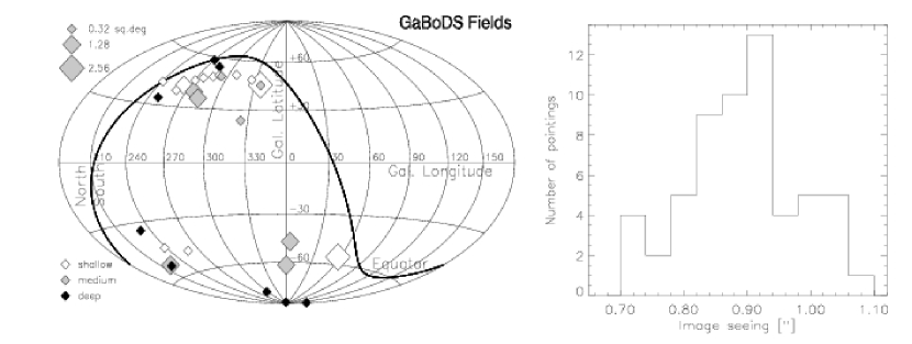
Figure 1: Left: Sky distribution of the GaBoDS fields. The size of the symbols indicates the covered sky area (not to scale), with one WFI shot covering 0.32 square degrees. All fields are at high galactic latitude. Right: Image seeing of the 58 coadded WFI@2.2 mosaics used for the lensing analysis. The average seeing is 0$.\!\!^{\prime\prime}$86.

In the present work we use the aperture mass statistics ($M_{\mathrm{ap}}$) (Schneider 1996, hereafter S96) and a derivative of it for the shear-selection of density peaks, based on 19 square degrees of sky coverage. The purpose of the work is to establish a suitable filter function for $M_{\mathrm{ap}}$, and then apply it to an (inhomogeneous) set of data. The sample returned is currently the largest sample of shear-selected cluster candidates, yet is dwarfed by the total number of galaxy clusters known.

The outline of this paper is as follows. In Sect. 2 we give an overview of the data used, concentrating on its quality and showing the usefulness for this analysis. Section 3 contains a discussion of our implemented version of $M_{\mathrm{ap}}$, particularily with regard to the chosen spatial filter functions. We also introduce a new statistics, deduced from $M_{\mathrm{ap}}$. In Sect. 4 we present and discuss our detections, and we conclude in Sect. 5.

Throughout the rest of this paper we use common weak lensing notations, and refer the reader to Bartelmann & Schneider (2001) and Schneider et al. (2006) for more details and technical coverage.

2 Observations, data reduction, data quality

2.1 The survey data

The GaBoDS was conducted with the wide field imager (hereafter WFI@2.2) of the 2.2m MPG/ESO telescope in the $R$-band. It is to about 80% a virtual survey, which means most of the data was not taken by us but collected from the ESO archive. There are five main data sources:

• The ESO Distant Cluster Survey, consisting of 12 pointings that have been selected because $z=0.5\dots 0.8$ cluster candidates have been identified in them using colour techniques. These exposures are rather shallow and we are thus insensitive to such distant objects (Fig. 8). Therefore, these fields do not impose a selection effect and qualify for our survey.

• Our ASTROVIRTEL project for data mining the ESO archive, which yielded 30 random pointings. As compared to the rest of the fields, many of them have unsuitable PSF properties, e.g. due to less careful focusing, so that we selected the 19 best fields. Details of this approach and its implementation are given in Schirmer et al. (2003) and Micol et al. (2004).

• The COMBO-17 data makes for the deepest survey part. Four of the five fields (S11, A901, SGP and FDF) contain known clusters.

• The EIS Deep Public Survey, contributing 9 empty fields.

• Our own observations of 13 empty fields.

The final sky coverage is 18.6 square degrees, spread over 58 fields which are suitable for our weak gravitational lensing analysis. The overall sky distribution of the fields is shown in Fig. 1, and further characteristics are summarised in Table 2.

2.2 Data reduction

For the reduction of this specific data set we developed a stand-alone, fully automatised pipeline (THELI), which we made freely available to the community. It is capable of reducing almost any kind of optical, near-IR and mid-IR imaging data. A detailed description of this software package is found in Erben et al. (2005), in which we investigate its performance on optical data. One of the main assets of this package is a very accurate astrometric solution that does not introduce any artificial PSF distortions into the coadded images.

The only difference between the current version of THELI and the one we used for the reduction of the survey data over the last years, is that for the image coaddition EISdrizzle was used, which is meanwhile replaced by Swarp. The latter method leads to a 4% smaller PSF in the final image in case of superb intrinsic image seeing as in our survey. The PSF anisotropy patterns themselves are indistinguishable between the two coaddition methods. Since the natural seeing variations (Fig. 1) in our images are much larger than those 4%, our analysis remains unaffected.

2.3 Image seeing and PSF properties

The image seeing and the PSF anisotropy are critical for weak lensing measurements. They dilute and distort the signal and determine how well the shape of the lensed galaxies can be recovered. As can be seen from Fig. 1, 80% of our coadded images have sub-arcsecond image seeing, and 20% are around 1$.\!\!^{\prime\prime}$0, with an average of 0$.\!\!^{\prime\prime}$86. Thus, we reach the sub-arcsecond seeing regime very well which is commonly regarded as mandatory for weak lensing purposes.

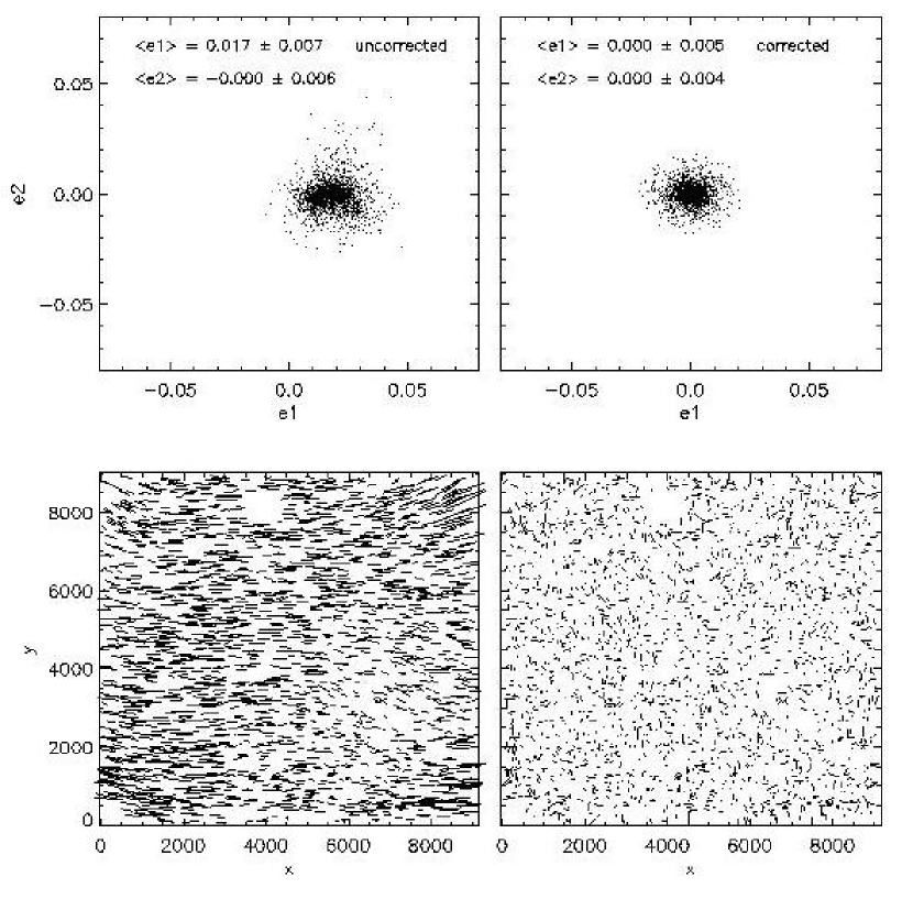
Figure 15: Typical PSF anisotropy. Upper row: $\varepsilon_{1,2}$ scatter plot for stars before and after PSF correction. Lower left: PSF anisotropy pattern before correction. This plot is a more intuitive representation of the left panel above. Lower right: PSF residuals after a polynomial fit was used to correct for the anisotropy. No coherent shear signal is left.

PSF anisotropies are rather small and usually well-behaved with WFI@2.2, which we have demonstrated several times (Schirmer et al. 2003, 2004; Erben et al. 2005, for example). With a well-focussed telescope, 1% of anisotropy in sub-arcsecond seeing conditions can be achieved, with a long-term statistical mode of around 2% (see Fig. 3). Discontinuities in the PSF are largely absent across chip borders. Slightly defocused exposures exhibit anisotropies of $3-5\%$. We rejected individual exposures from the coaddition if one or more CCDs had an anisotropy of larger than 6% in either of the ellipticity components $\varepsilon_{1}$ or $\varepsilon_{2}$. These anisotropies arise from astigmatism, and they flip by 90 degrees if one passes from an intrafocal to an extrafocal exposure (see Schirmer et al. 2003, for an example of this, and Fig. 15 for a typical PSF anisotropy pattern in our data).

Since such intra- and extrafocal exposures are roughly equally numbered for a larger set of exposures, anisotropies due to defocusing average out in the coadded images. Those have on average an anisotropy of $1-2\%$ with a similar amount in the rms (variation of the PSF across the field). This is illustrated in Fig. 2, where we show the combined PSF anisotropy properties for all coadded mosaic images. The left panel shows the uncorrected mean ellipticity components, having $\langle\varepsilon_{1}\rangle\,=0.0138$ and $\langle\varepsilon_{2}\rangle\,=-0.0002$. These anisotropies are small and become $|\langle\varepsilon_{1,2}\rangle|\,<0.001$ after PSF correction for all mosaics.

Figure 2: Left: The average $\varepsilon_{1,2}$ ellipticity components for the PSF of each mosaic, before PSF correction. The $\varepsilon_{2}$ component is symmetric around zero, whereas the $\varepsilon_{1}$ component scatters broader around a value of 1.4%. We do not show the corresponding plot after PSF correction, since all $|\varepsilon_{1,2}|<0.001$. Middle: The scatter of the two components around their average values. This indicates the deviation from a constant PSF anisotropy across the field and the noise level. Right: Same as in the middle, but after applying our PSF correction scheme. As a result, not only does $\langle\varepsilon_{1,2}\rangle$ get largely removed, also their rms is significantly lowered.

Figure 3: Characteristic PSF anisotropies $\left<|\varepsilon^{*}|\right>$ (modulus of the ellipticity of stars, averaged over the entire CCD) of 700 randomly chosen exposures for CCDs 1 and 8 of the WFI@2.2 detector mosaic. The remaining six CCDs have somewhat better properties. The exposure times were in the range of 300-500 seconds, and the zenith distances were smaller than 40 degrees. The differences between the distributions arise from slightly different spatial orientations with respect to the focal plane (the CCDs are confined within $\pm 20$ microns), thus responding differently to the focus. Anisotropies larger than $1-2\%$ are mostly due to an increasingly defocused instrument. The exposures used for this statistics were taken by a dozen different observers spread over more than a year, and give an idea of the quality of the archival data.

The middle plot of Fig. 2 shows the uncorrected rms values for $\langle\varepsilon_{1,2}\rangle$, i.e. the deviations of the PSF from a constant anisotropy across the field. The rms of both components peaks around 1% and is reduced by a factor of 2 after PSF correction (right panel). The tail of the distribution seen in the middle plot essentially vanishes.

To evaluate the remaining residuals from PSF correction more quantitatively, we calculated the correlation function between stellar ellipticity and shear before and after PSF correction (Fig. 4), separately for the various survey data sources and over all galaxy positions,

$$\langle\varepsilon_{1,2}^{*,{\rm pol}}\,\gamma_{1,2}\rangle=1/N\;\sum_{i=1}^{N}\varepsilon_{i\,1,2}^{*,{\rm pol}}(\mbox{\boldmath$\theta$})\,\gamma_{i\,1,2}(\mbox{\boldmath$\theta$})\;.$$ (1)

Here $\gamma_{1,2}$ are the PSF-corrected ellipticities of the galaxies which serve as an unbiased estimator of the shear, and $\varepsilon_{1,2}^{*,{\rm pol}}$ are the components of the PSF correction polynomial at the position $\theta$ of a galaxy. We find that the correlation between stellar PSF and shear is greatly reduced by the PSF correction, yet some non-zero residuals remain as we expected. Another test for residual systematics from PSF correction in the final lensing catalogues is the $M_{\mathrm{ap}}$ (defined in equation (3)) two-point cross-correlation function of uncorrected ellipticities of stars and corrected ellipticities of galaxies (see Fig. 5),

$$\langle M_{\mathrm{ap}}^{*}M_{\mathrm{ap}}^{\rm gal}\rangle=\sum_{i=1}^{N_{\rm fields}}\langle M_{\mathrm{ap}}^{*}M_{\mathrm{ap}}^{\rm gal}\rangle_{i}\;.$$ (2)

We find small non-zero residuals with different behaviour for the various survey parts. In particular, these residuals become increasingly non-zero with growing aperture size for our own observations and part of the ASTROVIRTEL fields. We will come back to these two points later during our analysis in Sect. 4, concluding that they do not affect our cluster detection method in a noticeable way.

To summarise, our PSF correction effectively takes out mimicked coherent shear patterns from the data, yet small residuals remain, which are much smaller than the coherent shear signal (a few percent) we expect from a typical cluster at intermediate redshift range ($z=0.1\dots 0.4$).

2.4 Catalogue creation: object detection and calculation of lensing parameters

Our catalogue production can be split into three parts, the object detection, the calculation of the basic lensing quantities, and a final filtering of the catalogue obtained. An absolute calibration of the magnitudes with high accuracy is not needed for this work since we are mostly interested in the shapes of the lensed galaxies but not in their fluxes. We adopted photometric standard zeropoints which bring us, conservatively estimated, to within $0.05-0.1$ mag of the real photometric zeropoint.

For the detection process we use SExtractor (Bertin & Arnouts 1996) to create a primary source catalogue. The weight map created during the coaddition (see Erben et al. 2005) is used in this first step, guaranteeing that the highly varying noise properties in the mosaic images are correctly taken into account. This leads to a very clean source catalogue that is free from spurious detections. The number of connected pixels (DETECT_MINAREA) used in this work for the object detection was 5, and we set the detection threshold (DETECT_THRESH) to 2.5. These thresholds are rather generous. $10-25\%$ of the objects detected are rejected again in the later filtering process since they were too small or too faint for a realiable shear measurement, or other problems appeared during the measurement of their shapes or positions.

In the second step we calculate the basic lensing quantities using KSB (Kaiser et al. 1995). This includes PSF anisotropy correction, and the recalculation of the objects’ first brightness moments since SExtractor yielded positions with insufficient accuracy for the purpose of our analysis. Details of our implementation of KSB are given in Erben et al. (2001), and a mathematical description of the PSF anisotropy correction process itself can be found in Bartelmann & Schneider (2001).

2.5 Catalogue creation: filtering

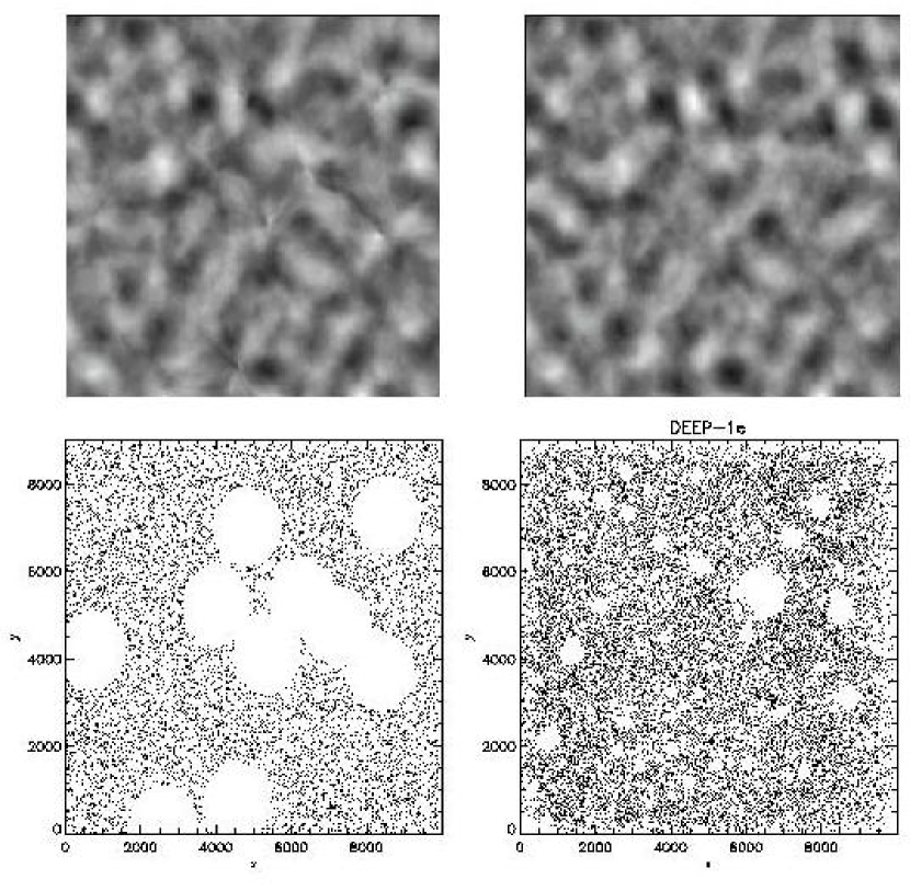
Figure 17: Upper right: $S$-map for randomised galaxy orientations and positions. Upper left: The same $S$-map, evaluated after 10 randomly positioned holes with a radius of 90% of the filter scale were cut into the data field (lower left). Artificial features show up in the $S$-map at the positions of the holes, the latter being exaggerated in number and size for better visualisation. Lower right: True galaxy distribution of the field from which the galaxies were drawn for this test. The largest hole is caused by an 8th magnitude star. We conclude that holes in the data fields are in general not a cause of concern for our analysis.

The third step consists of filtering the catalogue for various unwanted effects. To avoid objects in the catalogue that are in the immediate vicinity of bright stars, we explicitly set BACK_TYPE = MANUAL and BACK_VALUE = 0.0 (our coadded images are sky-subtracted) in the SExtractor configuration file. Thus SExtractor is forced to assume a zero sky background and does not model the haloes around bright stars as sky background. This proved to be a very efficient way of automatically masking brighter stars and the regions immediately surrounding them (see e.g. the lower right panel of Fig. 17). Further filtering on the SExtractor level is done by excluding all objects that are flagged with FLAG $>4$ and those with negative half-light radii.

Figure 4: Shown is the correlation between stellar ellipticity and measured shear before (left panel) and after (right panel) PSF correction for the 58 survey fields. The median improvement is a factor of 3, but residuals are still present.

Figure 5: $M_{\mathrm{ap}}$ two-point cross-correlation function of uncorrected ellipticities of stars and corrected ellipticities of galaxies, binned for the various survey data sources. The analysis of the ASTROVIRTEL fields has been split up into the B8- and C0-fields, since these exhibit different properties.

On the KSB level we filter such that only galaxies for which no problems in the determination of centroids occurred remain in the catalogue. Galaxies with half-light radii ($r_{\rm h}$) smaller than $0.1-0.2$ pixels than the left ridge of the stellar branch in an $r_{\rm h}$-mag-diagramme are rejected from the lensing catalogue, as are those with exceedingly bright magnitudes or a low detection significance ($\nu_{\rm max}<10$). See the left panel of Fig. 6 for an illustration of these cuts. From the same panel it can be seen that a significant number of galaxies have half-light radii comparable to or a bit smaller than the PSF, which makes their shape measurement noisier. Yet their number is large enough so that the shear selection of galaxy clusters profit significantly when these objects are included in the calculation. By including these objects, we gain $10-25\%$ in terms of the number density of galaxies, and $3-10\%$ in terms of signal-to-noise of the detections.

Furthermore, all galaxies with a PSF corrected modulus of the ellipticity larger than 1.5 are removed from the catalogue (the ellipticity can become larger than 1 due to the PSF correction factors, but is then downweighted), as are those for which the correction factor $({\rm Tr}\,P^{\rm g})^{-1}>5$ (see Erben et al. 2001). The fraction of rejected galaxies due to the cut-off in $P^{\rm g}$ is relatively small, as can be seen from the right panel in Fig. 6.

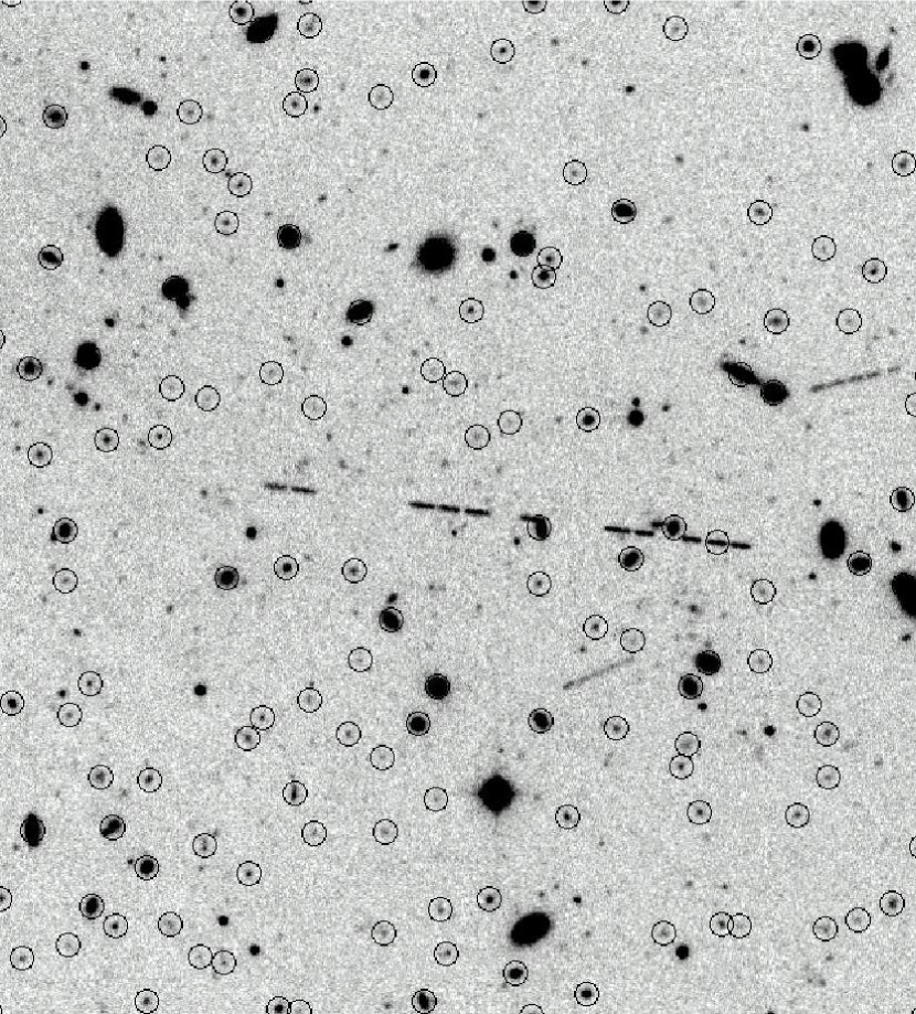
Figure 14: Indicated are the objects that are left over in the lensing catalogue after all typical filtering steps. Only fainter background galaxies are kept. Brighter sources, spurious detections, stars and highly elliptical objects such as asteroid tracks are largely absent from the catalogue. The field of view is about 3$\;\!\!{}^{\prime}\;$.

An overall impression of the remaining objects in the final catalogues is given in Fig. 14. In total, typically $10-25$% of the objects are rejected from the initial catalogue due to the KSB filtering steps. The remaining average number density of galaxies per field is $n\sim 11\;{\mathrm{arcmin}}^{-2}$ (min: 6, max: 28), not corrected for the SExtractor-masked areas (as described at the beginning of this section; on the order of 5% per field). For the width of the ellipticity distribution we measure $\sigma_{\varepsilon}=0.34$ for each of the two ellipticity components, averaged over all survey fields. Both $n$ and $\sigma_{\varepsilon}$ determine the signal-to-noise of the various mass concentrations detected.

3 Detection methods

3.1 S-statistics and an optimal filter Q

We base our detection method on the aperture mass statistics ($M_{\mathrm{ap}}$) as introduced by S96. $M_{\mathrm{ap}}$ can be written as a filtered integral of the tangential shear $\gamma_{\rm t}$,

$$M_{\mathrm{ap}}(\mbox{\boldmath$\theta$}_{0})=\int\mathrm{d}^{2}\varphi\;\gamma_{\rm t}(\mbox{\boldmath$\varphi$};\mbox{\boldmath$\theta$}_{0})\;Q(\varphi)\,.$$ (3)

Originally, the idea of $M_{\mathrm{ap}}$ is to obtain a measure of the mass inside an aperture independent of the mass sheet degeneracy in the weak lensing case. Written in the form (3) we can also simply interpret it as the filtered amount of the tangential shear around a fiducial point $\mbox{\boldmath$\theta$}_{0}$ on the sky, where $\gamma_{\rm t}(\mbox{\boldmath$\varphi$};\mbox{\boldmath$\theta$}_{0})$ is the tangential shear at position $\varphi$ relative to $\mbox{\boldmath$\theta$}_{0}$, and $Q$ is some radially symmetric spatial filter function.

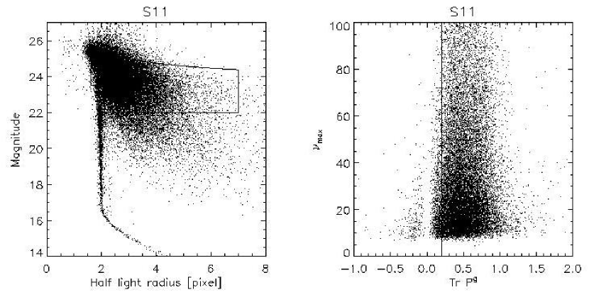
Figure 6: Left panel: Stars appear as a vertical branch in a $r_{\rm h}$-mag plot. Those brighter than $R=16.5$ saturate the detector and thus increase in size. The solid line encircles the galaxies which are used for the lensing analysis. The upper curved line indicates a cut in detection significance ($\nu_{\rm max}>10$), which has proven to work significantly better than a constant cut on the faint end of the magnitudes. Right panel: $\nu_{\rm max}$ against $P^{\rm g}$. Objects left of the indicated threshold are rejected from the lensing catalogue. Typically 1% of the galaxies are removed during this step.

The variance of $M_{\mathrm{ap}}$ for the unlensed case, respectively the weak lensing regime, is given by

$$\sigma^{2}_{M_{\mathrm{ap}}}=\frac{\pi\sigma_{\varepsilon}^{2}}{n}\int_{0}^{\theta}\mathrm{d}\vartheta\,\vartheta\,Q^{2}(\vartheta)\,,$$ (4)

where $\sigma_{\varepsilon}$ is the dispersion of intrinsic source ellipticities, and $n$ the number density of background galaxies. The integration is performed over a finite interval since we will have $Q\sim 0$ for $\vartheta>\theta$, i.e. for radii larger than the aperture size chosen. For the application to real data we will replace this integral in Sect. 3.2 by a sum over individual galaxies.

We then define the S-statistics, or the $S/N$ for $M_{\mathrm{ap}}$ respectively the measured amount of tangential shear, as

$$S(\theta;\mbox{\boldmath$\theta$}_{0})=\sqrt{\frac{n}{\pi\,\sigma_{\varepsilon}^{2}}}\;\frac{\int_{0}^{\theta}\mathrm{d}^{2}\vartheta\,\gamma_{\rm{t}}(\mbox{\boldmath$\vartheta$};\mbox{\boldmath$\theta$}_{0})\,Q(\vartheta)}{\sqrt{\int_{0}^{\theta}\mathrm{d}\vartheta\,\vartheta\,Q^{2}(\vartheta)}}\;.$$ (5)

Here $\theta$ is the aperture radius, and $\vartheta$ measures the distance inside this aperture from its centre at $\mbox{\boldmath$\theta$}_{0}$. This expression gets a bit simplified due to assumed radial symmetry (see Appendix A). Hereafter, we will call the 2-dimensional graphical representation of the $S$-statistics the S-map. If we plot the $S$-statistics for a given mass concentration as a function of aperture size, then we refer to this curve as the S-profile.

The filter function $Q$ that maximizes $S$ for a given density (or shear) profile of the lens can be derived using either a variational principle (Schirmer 2004), or the Cauchy-Schwarz inequality (S96). It is obtained for

$$Q(\vartheta)\propto\gamma_{\rm{t}}(\vartheta)\;,$$ (6)

where $\gamma_{\rm t}(\vartheta)$ is the tangential shear of the lens, averaged over a circle of angular radius $\vartheta$. This is intuitively clear, since a signal (i.e., $\gamma_{\rm{t}}$) with a certain shape is best picked up by a similar filter function ($Q$). We present in Sect. 3.4 a mathematically simple family of filter functions that effectively fulfills this criterion for the NFW mass profile.

3.2 Formulation for discrete data fields

For the application to real data, the previously introduced continuous formulation has to be discretised. First, we replace the tangential shear $\gamma_{\rm t}$ with the tangential ellipticity $\varepsilon_{\rm{t}}$, which is in the weak lensing case an unbiased estimator of $\gamma_{\rm t}$. Thus we have

$$M_{\mathrm{ap}}=\frac{1}{n}\sum_{i=1}^{N}\varepsilon_{{\rm t}i}\;Q_{i}\,,$$ (7)

where $n$ is the number density of galaxies, and $N$ the total number of galaxies in the aperture. Introducing individual galaxy weights $w_{i}$ as proposed by Erben et al. (2001), this becomes

$$M_{\mathrm{ap}}=\frac{A}{\sum_{i}w_{i}}\;\sum_{i}\varepsilon_{{\rm t}i}\;w_{i}\;Q_{i}\,,$$ (8)

where $A$ is the aperture area, previously absorbed in the number density $n$.

The noise of $M_{\mathrm{ap}}$ can be estimated from $M_{\mathrm{ap}}$ itself as was shown by Kruse & Schneider (1999) and S96. In the weak lensing case its variance evaluates as

$$\sigma^{2}(M_{\mathrm{ap}})=\langle{M_{\mathrm{ap}}}^{2}\rangle-\langle M_{\mathrm{ap}}\rangle^{2}\ =\langle{M_{\mathrm{ap}}}^{2}\rangle\;,$$ (9)

since one expects $\langle M_{\mathrm{ap}}\rangle=0$. Substituting with equation (7) yields

$$\sigma^{2}(M_{\mathrm{ap}}) = \frac{1}{n^{2}}\;\sum_{i,j}\langle\varepsilon_{{\rm t}i}\,\varepsilon_{{\rm t}j}\rangle\,Q_{i}\,Q_{j}=\frac{1}{n^{2}}\;\sum_{i}\langle{\varepsilon_{{\rm t}i}}^{2}\rangle\,{Q_{i}}^{2}$$ (10)

$$= \frac{1}{2n^{2}}\;\sum_{i}|\varepsilon_{i}|^{2}\,{Q_{i}}^{2}\,,$$

where we used

$$\langle{\varepsilon_{{\rm t}}}^{2}\rangle=\frac{1}{2}\,|\varepsilon|^{2}\;,$$ (11)

and the fact that $\varepsilon_{{\rm t}i}$ and $\varepsilon_{{\rm t}j}$ are mutually independent and thus average to zero for $i\neq j$. The $Q_{i}$ are constant for each galaxy and thus can be taken out of the averaging process. Again, in the case of individual galaxy weights this becomes

$$\sigma^{2}(M_{\mathrm{ap}})=\frac{A^{2}}{2\;\left(\sum_{i}w_{i}\right)^{2}}\;\sum_{i}|\varepsilon_{i}|^{2}\;w_{i}^{2}\;Q_{i}^{2}\,,$$ (12)

using the fact that the $w_{i}$ are constant for each galaxy like the $Q_{i}$. Therefore, we obtain for the $S$-statistics

$$S=\frac{\sqrt{2}\;\sum_{i}\varepsilon_{{\rm t}i}\,w_{i}\,Q_{i}}{\sqrt{\sum_{i}|\varepsilon_{i}|^{2}\,w_{i}^{2}\,{Q_{i}}^{2}}}\;,$$ (13)

which grows like $\sqrt{N}$.

3.3 Validity of the $M_{\mathrm{ap}}$ concept for our data

If $M_{\mathrm{ap}}$ is evaluated close to the border of an image or on a data field with swiss-cheese topology due to the masking of bright stars, then the aperture covers an ‘incomplete’ data field. Therefore, the returned value of $M_{\mathrm{ap}}$ does no longer give a result in the sense of its original definition in S96, which was a measure related to the filtered surface mass density inside the aperture. Yet it is still a valid measure of the tangential shear inside the aperture, including the $S/N$-estimate in equation (13), and can thus be used for the detection of mass concentrations.

Since the number density of background galaxies inside an aperture is not a constant over the field due to the masking of brighter stars (and the presence of the field border), we have to check for possible unwanted effects. As long as the holes in the galaxy distribution are small compared to the aperture size, and as long as their number density is small enough so that no significant overlapping of holes takes place, the effects on the $S$-statistics are negligible (see Fig. 17). In fact, the decreased number density just leads to a lowered significance of the peaks detected in such areas, without introducing systematic effects.

If the size of the holes becomes comparable to the aperture, spurious peaks appear in the $S$-map at the position of the holes. This is because the underlying galaxy population changes significantly when the aperture is moved to a neighbouring grid point. When such affected areas were present in our data, then we excluded them from the statistics and masked them in the $S$-maps, even though these spurious peaks are typically not very significant ($\sim 2\sigma$). Our threshold for not evaluating the $S$-statistics at a given grid point is reached if the effective number density of the galaxies in the aperture affected is reduced by more than 50% due to the presence of holes (or the image border). Spurious peaks become very noticeable if the holes cover about 80% of the aperture. This is rarely the case for our data unless the aperture size is rather small (2$\;\!\!{}^{\prime}\;$), or a particular star is very bright. We conclude that our final statistics is free from any such effects.

3.4 Filter functions

As expressed in (6), an optimal filter function should resemble the tangential shear profile. In the following such a filter $Q(x)$ is constructed, assuming that the azimuthally averaged shear dependence is caused by an NFW density profile (Navarro et al. 1997) of the lensing mass concentration. We set $x:=\vartheta/\theta$, with $x$ being the projected angular separation $\vartheta$ on the sky from the aperture centre, in units of the aperture radius $\theta$. By varying $\theta$, shear patterns respectively mass concentrations of different extent can be detected.

Wright & Brainerd (2000) and Bartelmann (1996) derived an expression for the tangential shear of the universal NFW profile. Based on their finding we can construct a new filter function $Q_{\rm NFW}$ over the interval $x\in[0,1]$, having the shape

$$Q_{\rm NFW}(x)=\;\;\;\;\;\;\;\;\;\;\;\;\;\;\;\;\;\;\;\;\;\;\;\;\;\;\;$$ (14)

$$\begin{cases}\frac{4(3y^{2}-2)}{y^{2}(y^{2}-1)\sqrt{1-y^{2}}}\;{\rm{arctanh}}\sqrt{\frac{1-y}{1+y}}+\frac{4}{y^{2}}\,{\rm{ln}}\frac{y}{2}+\frac{2}{1-y^{2}}&\;\;(y<1)\\[8.5359pt] \frac{10}{3}-4\,{\rm{ln}}\,2&\;\;(y=1)\\[4.26773pt] \frac{4(3y^{2}-2)}{y^{2}(y^{2}-1)\sqrt{y^{2}-1}}\;{\rm{arctan}}\sqrt{\frac{y-1}{1+y}}+\frac{4}{y^{2}}\,{\rm{ln}}\frac{y}{2}+\frac{2}{1-y^{2}}&\;\;(y>1)\end{cases}\;$$

Here we defined $y:=x/x_{\rm c}$, with $x_{\rm c}$ being a dimensionless parameter changing the width (and thus the sharpness) of the filter over the interval $x\in[0,1]$, in the sense that more weight is put to smaller radii for smaller values of $x_{\rm c}$. This expression is smooth and continuous for $y=1$, and approaches zero as ${\rm ln}(y)/y^{2}$ for $y\gg 1$.

Figure 7: Left panel: $Q_{\rm NFW}$ (solid line), shown with some representations of $Q_{\rm TANH}$. The exponential cut-off $E(x)$ for small and large radii is not introduced in this plot in order to show the differences between the two filter types better. As can be seen, the $Q_{\rm TANH}$ filter is a very good approximation for $Q_{\rm NFW}$, giving slightly more weight to smaller radii. Right panel: $Q_{\rm TANH}$ with the cut-off introduced by $E(x)$ at both ends, plotted against the radial coordinate $\vartheta$. The dashed line ($\theta=1$) can be compared directly to the dash-dotted line in the left panel.

Due to the mathematical complexity of $Q_{\rm NFW}$, the calculation of the $S$-statistics is rather time consuming for a field with $\sim 10^{4}$ galaxies. We introduce an approximating filter function with simpler mathematical form that produces similarly good results as $Q_{\rm NFW}$. It is given by

$$Q_{\rm TANH}(x)=E(x)\;\frac{{\rm tanh}\,(x/x_{\rm c})}{x/x_{\rm c}},$$ (15)

having the $1/x$ dependence of a singular isothermal sphere for $x\gg x_{\rm c}$. The hyperbolic function, having a $\propto x$ dependence for small $x$, absorbs the singularity at $x=0$ and approaches 1 for growing values of $x$. The pre-factor $E(x)$ is a box filter, independent of $x_{\rm c}$, with exponentially smoothed edges. It reads

$$E(x)=\frac{1}{1+{\rm e}^{6\,-\,150x}+{\rm e}^{-47\,+\,50x}}$$ (16)

and lets $Q$ drop to zero for the innermost and outermost 10% of the aperture, while not affecting the large rest (see right panel of Fig. 7). It is introduced because both $Q_{\rm NFW}$ and $Q_{\rm TANH}$ (without this pre-factor) are not zero at the centre nor at the edge of the aperture. This cut-off is very similar to that introduced in [S96] for a different radial filter profile. It suppresses stronger fluctuations when galaxies enter (or leave) the aperture, receiving significant non-zero weight. It also avoids assigning a large weight to a few galaxies at the aperture centre, which as well can lead to significant fluctuations in the $S$-statistics when evaluated on a grid. The effect of $E(x)$ is rather mild though, since usually several hundred galaxies are covered by one aperture unless it is of very small size so that $E(x)$ becomes important.

We thus have a filter function based upon the two-dimensional parameter space $(\theta\,,x_{\rm c})$. The differences between $Q_{\rm TANH}$ and $Q_{\rm NFW}$ are indistinguishable in the noise once applied to real data, so that we do not consider $Q_{\rm NFW}$ henceforth.

It is not the first time that $M_{\mathrm{ap}}$ filters following the tangential shear profile are proposed or used. We have already utilised the filter in equation (15) to confirm a series of luminosity-selected galaxy clusters (Schirmer et al. 2004). Before that, Padmanabhan et al. (2003) approximated $Q_{\rm NFW}$ with

$$Q_{\rm PAD}(x)=\frac{2\;{\rm ln}(1+x)}{x^{2}}-\frac{2}{x(1+x)}-1/(1+x)^{2}\;,$$ (17)

which was later-on modified by Hennawi & Spergel (2005). They multiplied (17) with a Gaussian of certain scale radius in order to suppress the effects of the cosmic shear that become dominant for larger radii. Even though the mathematical descriptions are different, the latter two filters are in effect very similar to (15), and we could not find one of them superiour over the other based on our rather inhomogeneous data set. Hence, we do not consider them for the rest of the work. The validity of our approach has recently been confirmed by Maturi et al. (2006), who also use a filter following the tangential shear profile, individually adapted for each field to minimise the effect of cosmic shear. Based on the same data as we use in the present paper, they find that our filter defined in equation 15 yields very similar results as compared to their optimised filter, which means that the lensing effects of the large scale structure in our rather shallow survey are not very dominant.

Differences in the efficiency of such “tangential” filters are thus expected to arise for very deep surveys only, and/or in case of high redshift clusters ($z=0.6$ and more, for which our survey is not sensitive). In all other cases they are hardly distinguishable from each other since the noise in the images and the deviations from the assumed radial symmetry of the shear field and the NFW profile are dominant. Thus we consider the $Q_{\rm TANH}$ filter to be optimally suited for our survey. For a comparison with other filters that do not follow the tangential profile, see the example shown in Fig. 16.

Figure 8: Expected optimal S/N ratios for NFW dark matter haloes for four different cluster masses ($M_{200}$) and two different image depths. The mathematical derivation of the $S/N$ for a particular cluster at a given redshift is given in Appendix A. Note that the filter scale is not constant along each of the curves since the shear fields get smaller in angular size with increasing lens redshift. Note also that we used a lower integration limit of $z_{\rm d}=0.2$ for the lensed background galaxies (see Sect. 3.5 for both aspects).

3.5 Sensitivity

Figure 8 gives an idea of the sensitivity of our selection method for the $Q_{\rm TANH}$ filter (see Appendix A for mathematical details). This plot was calculated taking into account various characteristics of our survey and analysis. First, we introduced a maximum aperture radius of 20$\;\!\!{}^{\prime}\;$to reflect the finite field of view of our fields. This affects (lowers) the $S/N$ of very low redshift ($z<0.09$) clusters, whose shear fields can be very extended, and leads to a more distinct maximum of the curves. Second, the aperture size is not a constant along these curves but limited by the angular distance where the strength of the tangential shear drops below 1%, merging into the cosmic shear. Lastly, we used a lower redshift cut-off of $z_{\rm d}=0.2$ in order to roughly reflect our selection criteria for the background galaxies (see Fig. 6). The effect of the latter cut is minor, it increases the $S/N$ on the order of 5% for the low redshift range we probe, as compared to no cut.

As a result, our $S$-statistics is insensitive for structures of mass equal or less than $M_{200}=5\times 10^{13}$ M_⊙ for all redshifts. In data of average depth ($n=12\;{\mathrm{arcmin}}^{-2}$) we can detect mass concentractions of $1,2,4\times 10^{14}$ M_⊙ out to $z=0.10,0.22$ and 0.32, respectively. The same objects would still be seen at $z=0.22,0.34$ and 0.46 in the deeper exposures with twice the number density of usable background galaxies.

3.6 Introducing the $P$-statistics

In addition to the $S$-statistics defined above, we introduce a new measure which we call peak position probability statistics, hereafter simply referred to as P-statistics. It tells us if at one particular position on the sky the $S$-statistics makes significantly more detections for various filter scales than one would expect in the absence of a lensing signal. As we find in Sect. 4, the $S$- and $P$-statistics complement each other rather well.

We calculate the $P$-statistics as follows:

• For each given survey field we look up the positions of all peaks detected in the full $(\theta\,,x_{\rm c})$ parameter space.

• We then select all positive peaks with a signal-to-noise larger than 2.5, and map their positions on the sky. The individual positions are weighted with the corresponding peak $S/N$. This discrete map is then smoothed with a Gaussian kernel of width 40$\;\!\!{}^{\prime\prime}\;$, yielding a continuous map. The smoothing is introduced to smooth out the variations in the positions determined for the very same peak using different filter scales. In other words, it links two detections made nearby on the sky in different filters to the same mass concentration.

• We randomise the orientations of the galaxies in the original catalogue 10 times and repeat the above step. From that we derive a constant noise level for each survey field. The assumption of a constant noise is an approximation which we based on a set of 200 randomisations of an arbitrary survey field. We find that the noise is constant to within 15% or less. It can be well estimated with a set of just 10 randomisations.

• The “true” map is then divided by the rms obtained from the noise map, yielding an estimate of how reliable the peak at the given position is. We then call this rescaled map the $P$-map in analogy to the $S$-map. However, note that the $P$-statistics has a very non-Gaussian probability distribution function (see also the left panel of Fig. 9).

The main idea behind this approach is that a real peak has an extended shear field, i.e. it will be picked up by a larger number of different filter scales. In other words, as the aperture size changes, different samples of galaxies are used and all of them will yield a signal above the detection threshold (provided a sufficient lensing strength). On the contrary, a spurious peak mimicked by the noise of the intrinsic galaxy ellipticity is not expected to show such a behaviour, thus the $P$-statistics will prefer a true peak over a false peak. It has an advantage over the $S$-statistics since it looks at a broader range of filter scales instead of one single scale. Thus it is capable of giving significance to a peak that otherwise goes unnoticed by the $S$-statistics. On the other hand, objects with weak shear fields will not be recognised by the $P$-statistics since they appear only for one or a few nearby filter scales.

We would like to emphasise that we introduced the $P$-statistics for this work on an experimental basis only. Its performance has not yet been evaluated based on simulations, but it yields very similar results as the $S$-statistics (see Sect. 4), so that we included it in this presentation.

There is some arbitrariness in the way we implemented the $P$-statistics. For example, the lower threshold of 2.5$\sigma$ for the peaks considered can be decreased or increased. The former would make it smoother since more peaks are included, but does not yield any further advantage since it picks up too much noise. Increasing the threshold beyond 3.5 reduces the number of peaks entering the statistics significantly. This makes the determination of the noise level unstable, and one starts losing less significant peaks. There is also room for optimisation concerning the selection of input data, as for this work we simply included peaks from the full parameter space. Concentrating on a smaller set of filter scales could yield a more discriminative power, but bears the risk of losing objects. In addition, the smoothing length has been chosen to obtain the best compromise between smoothing out position variations in the lensing detections while maintaining the spatial resolving power of the $P$-statistics. The chosen kernel width of 40$\;\!\!{}^{\prime\prime}\;$appears optimal for our survey, but may well be different for other data sets.

In order to distinguish between individual $S/N$ measurements made with the $P$- and $S$-statistics, we will use the terms $\nu_{\mathrm{p}}\,$and $\nu_{\mathrm{s}}\,$henceforth.

Figure 9: Left panel: The normalised PDF for the peaks based on the entire survey area, averaged over all scales and $x_{\rm c}$. Whereas the peak PDF for the $S$-statistics can be well approximated by a Gaussian, the PDF for the $P$-statistics is highly non-Gaussian with a broad tail. The $\nu_{p}$ should therefore not be directly interpreted as $S/N$. The middle ($S$-statistics) and right panel ($P$-statistics) show the difference between the observed peak PDF and the PDF obtained from 10 randomisations. The middle plot is magnified by $\times 100$ for $|\nu_{s}|\geq 4$ for better visualisation. Both these plots also contain the minimum (and mostly negative) peaks, i.e. underdense regions or voids, which accounts for the symmetric appearance. A significant excess of peaks and voids exists in the observed data (as compared to the randomised data) for $|\nu_{s}|>2$ and $|\nu_{p}|>3$. The error bars are taken from the randomisations.

3.7 Validation of the $S$- and $P$-statistics

As a consistency check for the concept of the $S$- and the $P$-statistics, one can compare the peak probability distribution function (PDF) of the observed data against randomised data sets. The presence of cluster lensing should distort the PDF in the sense that more peaks are detected for higher $S/N$ values (see Miyazaki et al. 2002, for an example).

To this end we created 10 copies of our entire survey catalogue with randomised galaxy orientations, destroying any lensing signal, but keeping the galaxy positions and thus all other data characteristics fixed. We then calculated the PDFs for all local maxima (overdense regions) and minima (underdense regions) of the observations and the randomisations, accumulating the detections from the entire parameter space probed. The middle and right panel of Fig. 9 show the difference between the PDFs of the observed and the randomised data sets. Both PDFs, for the $S$- and the $P$-statistics, are significantly skewed, showing an excess of peaks and voids above thresholds of about $\nu_{s}>2$ and $\nu_{p}>3$.

4 Shear-selected mass concentrations

4.1 Selecting the cluster candidates

The way we established our sample of possible mass concentrations (“peaks”) is as follows. The $S$-statistics is evaluated

• on a grid with a 10$\;\!\!{}^{\prime\prime}\;$spacing

• for 19 different filter scales.

• for 7 different scale parameters $x_{\rm c}$

• From these $S$-maps (133 different representations per survey field) we include all peaks higher than 4$\sigma$, which corresponds to the lower limit of the $(S/N)_{\rm min}=4\dots 5$ range that is considered useful by various authors (see Reblinsky & Bartelmann 1999; Hamana et al. 2004, for example).

The $P$-statistics is evaluated on the same grid space and obtained as described in Sect. 3.6. We will use as well a detection threshold of $\nu_{p}=4.0\sigma$, which has shown to provide us with a similar number of detections as the $S$-statistics, so we can compare the two samples.

The detections made with both statistics are summarised in Tables 3 to 5. Those peaks seen with the $S$-statistics have the best matching filter scale reported, i.e. the one yielding the highest $S/N$. Column 1 contains numeric labels for the detections, followed by a string indicating with which statistics it was made. The third and fourth column contain the detection significances $\nu_{\mathrm{p}}\,$and $\nu_{\mathrm{s}}\,$(if applicaple). Columns five, six and seven carry a classification parameter (see below), a richness estimate of a possible optical counterpart if present, plus the distance of the peak from the latter. This is followed by the filter scale and the $x_{\mathrm{c}}$ parameter (if applicable), and then the name of the survey field in which the detection was made. Finally, we report the redshift of an optical counterpart if known.

4.2 Classification of the peaks detected

In order to characterise the line of sight for a peak in terms of visible matter, we introduce a rough classification scheme based on the $R$-band images. We visually inspected a radius of 2$.\!\!^{\prime}$0 around the peak position for apparent overdensities of brighter galaxies, as compared to the surrounding field. Even though this is a rather crude approach, it is good enough to tell if a peak is likely associated with some luminous matter, or not. The radius of 2$.\!\!^{\prime}$0 has been chosen since we observed from known galaxy clusters that the lensing detection can scatter up to 1$.\!\!^{\prime}$5 with respect to the optical center of the cluster (see Table 1). This is either due to substructure in the cluster, or due to noise (the detection is made from a finite number of galaxies only).

The classes are defined as follows and are based on galaxies taken from the range $R\sim 17-22$ (thus they are not member of the catalogue of background galaxies, see also the left panel of Fig. 6):

• class 1: concentration of more than 50 galaxies

• class 2: 35-50 galaxies

• class 3: 25-35 galaxies

• class 4: 15-25 galaxies

• class 5: 5-15 galaxies

• class 6: no counterpart visible

Judging from our number counts (Hildebrandt et al. 2006) for the ESO Deep Public Survey data, we expect a number density of about 11000 galaxies with $R\leq 22$ per square degree. Assuming a random distribution of these foreground galaxies and neglecting clustering effects, we obtain a scattering of $\sigma=7.2$ for the total number of galaxies within the 2 arcmin radius. Thus, class 5 objects represent not more than a 2.1$\sigma$ overdensity as compared to the randomised distribution.

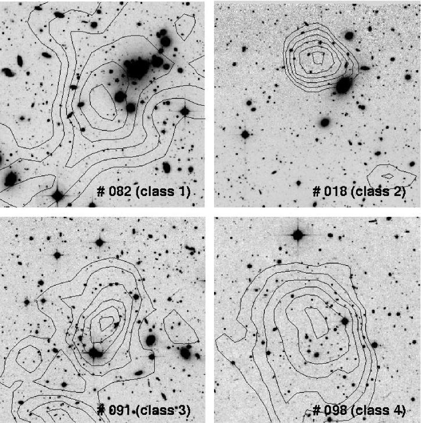
Figure 18: Illustrates the typical appearance of bright clusters of various classes, as defined in Sect. 4.2. Note that the resolution is in general not high enough to distinguish smaller member galaxies from stars. The field of view is 4$.\!\!^{\prime}$3.

We consider classes 1 to 4 to be reliable optical counterparts, and refer to them as bright peaks henceforth. Classes 5 are rather dubious, and go as dark peaks together with those lines of sight classified as 6. See Fig. 18 for an illustration of bright peaks of classes $1-4$.

The boundaries between the classes are permeable. For example, if we find an overdensity of 12 galaxies, and 4 or 5 of them stand out from the rest by their brightness and are of elliptical type, the class 5 object would become a class 4. Similarly, if we find 20 galaxies of similar brightness, but they show a significantly higher concentration than the rest of the sample, it becomes class 3. On the other hand, if the distance between the mass peak and the center of the optical peak exceeds 100 arcseconds, we decrease the class by one step. The same holds if the galaxies seen appear to be at redshift higher than $\sim 0.3$ or more, then we lower the rank by 1 since our selection method becomes less sensitive with increasing redshift. About 20% of our sample were up- or downgraded in this way.

4.3 Spectroscopically “confirmed” candidates

For 22 out of the 72 bright peaks, we found spectra in the NASA Extragalactic Database. Most of them come from the SDSS or the Las Campanas Distant Cluster Survey (Gonzalez et al. 2001). For 7 cases we have only two spectra, thus they just indicate a cluster or group nature, but we can not take it as hard evidence. Those redshifts are marked with an asterisk in Tables 3 to 5. For 15 other peaks the cluster nature was already known or has meanwhile been secured, either by spectroscopy, photometric redshifts, or by other photometric means (see e.g. Gladders & Yee 2000, for the red sequence method). Three of them (#043, 053 and 157) turn out to be clusters or groups of galaxies at different redshifts projected on top of each other, with the previous two being triple. For simplicity, we refer to all these objects in the following as “confirmed” peaks, even though more spectroscopic data has to be obtained for most of them for sufficient evidence.

Whenever spectra were available, they confirmed our assumption of spatial concentrations in all cases. In order to secure the 50 most promising candidates, we recently started a large spectroscopic survey aiming at between 20 and 50 galaxies per target. This will not only pin down the redshifts of the possible clusters, but also allow us to identify further projection effects and in some cases possible physical connections with nearby peaks (e.g. #029, 056, 074, 084, 092, 128, 136, 141, 158). We will report these results in future papers.

The $1\sigma$ redshift range of the peaks confirmed so far is $z=0.09\dots 0.31$. We therefore predominantly probe the lower redshift range of clusters, which is consistent with the theoretically expected sensitivity of our survey (see Kruse & Schneider 1999, and Fig. 8).

Table 1: Average angular offsets between the peak and the optical counterpart

class	number	average
	of peaks	offset [ $\;\!\!{}^{\prime\prime}\;$]
1	3	$53\pm 38$
2	14	$59\pm 24$
3	21	$51\pm 16$
4	34	$55\pm 30$
5	43	$62\pm 32$
6	43	N/A

4.4 Positional offsets

Table 1 shows that the peaks coincide with the positions of the optical counterparts to within 0$.\!\!^{\prime}$9$\pm$0$.\!\!^{\prime}$5, independent of the peak classification. On the one hand, these offsets are due to noise, since the shear field is obtained by a finite number of lensed galaxies with intrinsic ellipticities. In addition, in general the shear fields deviate from the radial symmetry assumed by the $M_{\mathrm{ap}}$ filter. On the other hand, these offsets can be physical in the sense that light does not trace mass very well for young or still non-virialised clusters. The two largest clusters in our sample, Abell 901 (#039) and Abell 1364 (#082), are good examples. For them, the positions of the weak lensing detections are shifted away from the cD galaxies in the direction of sub-clumps. See also Fig. 18 for an illustration.

Figure 10: Shown is the spatial distribution of the 158 detected peaks for the WFI field of view. Open symbols indicate the bright peaks with classes 1-4, the filled ones peaks with classes 5 and 6. The symbol size represents the detection significance. The pattern is indistuinguishable from a random distribution, and we also do not see differences for peaks obtained with either the $S$- or the $P$-statistics (not shown).

Figure 11: Shows the fraction of detections made in either the $S$- or the $P$-statistics, or in both.

4.5 Comparing the $S$- and $P$-statistics

We make 90 and 95 detections with the $S$- and the $P$-statistics, respectively, having 26 peaks in common. As can be seen from Table 7, the number of bright and dark peaks is equally balanced between the two methods, both yielding slightly more dark than bright peaks. A few fields exist in which either only the $S$-statistics (e.g. CL1216-1201) or the $P$-statistics (e.g. FIELD17_P3) make detections, but the individual number of detections made per field are in general small. The statistics do not show a preference with respect to particular fields. The same holds for the spatial distribution of peaks as a function of position in the detector mosaic (see also Fig. 10), or the occurrence of dark peaks as a function of exposure time (see Fig. 12 for a merged plot of the two statistics). In general, the overlap between the two statistics increases if the detection thresholds of $S/N=4$ are further lowered, i.e. peaks seen in only one of the statistics then appear also in the other. Yet then the overall number of detections increases to many hundreds, and we did not evaluate the overlapping fraction in this case.

The only noteworth difference between the $S$- and the $P$-statistics is that the latter detects about 30% peaks of classes 2 and 3, whereas the $S$-statistics returns 25% more peaks of class 4. The occurence of dark peaks is indistuinguishable between the two methods (see Fig. 11).

4.6 Detector and survey field biases, dark peaks

To check for systematics concerning the WFI@2.2 detector array, we plotted the positions of all peaks with respect to the array geometry (Fig. 10). It appears that the right half is a bit more crowded than the left part of the detector array. After running a dozen random distributions with the same number of objects we find that this is insignificant. Thus the distribution is random-like for both bright and dark peaks, and does not prefer or avoid particular regions.

Upon counting the bright and dark peaks in the five main data sources of our survey (see Sect. 2.1), we find differences in the ratio between bright and dark peaks (Table 6). Namely, the ASTROVIRTEL and EIS data, and our own observations, show an excess of $20-50\%$ in terms of dark peaks as compared to the bright peaks, and are about comparable to each other. The EDisCS survey has a factor 2.1 more dark peaks, but is also that part of our survey with the most shallow exposure times. Contrary, the COMBO-17 data has twice as many bright as darks peaks, but this comes not as a surprise since the S11 and A901 fields are centered on known galaxy clusters with significant sub-structure. If we subtract the known clusters and all detections likely associated with them, we still have an “excess” of 40% for the bright peaks in COMBO-17. Again, this is not unplausible since the COMBO-17 fields form by far the deepest part of our survey, which let us detect more mass concentrations. But this holds for both bright and dark peaks, as the number of detections per square degree shows (Table 6).

In order to check if the dark peaks might arise due to imperfect PSF correction, we compare their occurrence with the remaining PSF residuals in our lensing catalogues (Figs. 4 and 5). Therein we do not find evidence that the imperfect PSF correction gives rise to dark peaks. However, Fig. 12 indicates that small exposure times (less than $10-12$ ksec) and/or a low number density (less than $n\sim 13-15\;{\mathrm{arcmin}}^{-2}$) of galaxies foster the occurrence of dark peaks. Yet this has to be seen with some caution, in particular because we have only a small number of deep fields (mainly COMBO-17) as compared to the shallow ones, and the deep fields are prtially concentrated on known structures. If we take the known structures into account and remove them from the statistics, we are still left with a smaller fraction of dark peaks in the deep exposures, but the question remains in how far the particular pointings of those fields introduce a bias. To answer this question empirically, we would need about 10 empty fields of 20 ksec exposure time each.

Due to the $M_{\mathrm{ap}}$ filter we use, and to the large inhomogeneity of our survey, we can not directly compare the occurrence of dark peaks in our data to existing numerical simulations. Also, these simulations usually make significantly more optimistic assumptions in terms of usable number density of galaxies and field of view than we could realise with GaBoDS (see Reblinsky & Bartelmann 1999; Jain & van Waerbeke 2000; Hennawi & Spergel 2005, for example). In particular Hamana et al. (2004) have shown that in their simulations ($n=30$) they expect to detect 43 real peaks (efficiency of $\sim 60\%$), scaled to the same area as GaBoDS and drawn with $S/N>4$ from mass reconstruction maps. A similar number of false peaks appear as well, being either pure noise peaks, or peaks with an expected $S/N<4$ being pushed over this detection limit. The latter would be labelled as bright peaks in our case. Our absolute numbers are different (72 bright and 86 dark peaks) since we use a very different selection method. Yet, if we interpret our dark peaks as noise peaks, the ratio between our bright and dark peaks is comparable to the ratio between their true and false peaks.

This interpretation, i.e. dark peaks are mostly noise peaks, is strengthened by the fact that with increasing peak $S/N$ the fraction of dark peaks is decreasing (see Table 7), for both the $S$- and the $P$-statistics. However, our observational data base (sky coverage) is too small to tell if this trend, i.e. the dark peaks dying out, continues for higher values of the $S/N$.

Figure 12: Shown is the number of bright peaks (solid line) and dark peaks (dashed line) as a function of exposure time (left) and galaxy number density (right). Shallow exposures with low number density have more dark peaks than deeper exposures.

Figure 13: Left: Histogram of the exposure times. The peak at 57 ksec represents the Chandra Deep Field South (CDF-S). Right: Number density of galaxies in the 58 fields after all filtering steps, leaving a total number of about 710000 usable galaxies. The distribution reflects the distribution of exposure times shown in the left panel.

5 Summary

In the present paper we have introduced a new type of filter function for the aperture mass statistics. This filter function follows the tangential shear profile created by a radial symmetric NFW density profile. We have shown that it is optimally suited for an application to our 19 square degree weak lensing survey conducted with the WFI@2.2m MPG/ESO telescope. This is a survey with very inhomogeneous depth, in which we expect to be able to detect mass concentrations in the redshift range $z=0.1\dots 0.5$. We also introduced the new $P$-statistics, currently on a test-basis only. It turned out to deliver very similar results in the number of bright and dark peaks detected, and for the time being looks like a good complement to the $S$-statistics. Its performance has to be investigated more deeply though, and there is space for optimisation. The global PDFs for both the $S$- and $P$-statistics show clear excess peaks for higher values of $S/N$ as compared to the randomisations. Thus the presence of lensing mass concentrations in our survey data is confirmed.

We introduced a classification scheme in order to associate the hypothetical mass peaks detected with possible luminous matter. From the 158 detections we made with the combined $S$- and $P$-statistics, 72 (46%) appear to have an optical counterpart. For 22 of those we found spectra in the literature, confirming the above mentioned redshift range, and that indeed a mass concentration exists along those particular lines of sight. For a smaller number of those we have spectroscopic evidence that the peaks detected are due to projection effects. We expect that in our currently conducted spectroscopic follow-up survey more such projection cases will be uncovered, together with a confirmation of a very significant fraction of the remaining bright peaks. In a future paper we will also compare this shear-selected sample with an optically selected sample using matched filter techniques.

We gained some insight into the subject of dark peaks. They appear preferentially in shallow data with a small number density of galaxies, indicating that a large fraction of those could be due to noise (i.e. instrinsic galaxy ellipticies), or they are statistical flukes. Nevertheless, in our deep fields we also observe a significant fraction of dark peaks, but our statistics can not be unambiguously interpreted since those fields are biased towards clusters with significant sub-structure, and we have only a very small number of them. Nevertheless, real physical objects such as very underluminous clusters are far from being ruled out at this point. At least on the mass scale of galaxies the last year has seen astonishing examples of objects having several $10^{8}\;M_{\odot}$ of neutral hydrogen, yet apparently no star formation has taken place in them (Minchin et al. 2005; Auld et al. 2006). Whether similar objects can still exist on the cluster mass scale is unclear.

Finally, we would like to repeat that the Garching-Bonn Deep Survey has been made with a 2m telescope. Most numerical simulations done so far are much more optimistic in terms of the number density reached ($n\sim 30\;{\mathrm{arcmin}}^{-2}$) and correspond to surveys that are currently conducted (or will be in the near future) with 4m- and 8m-class telescopes, such as SUPRIME33 (Miyazaki et al. 2005) or the CFHTLS. One noteworthy exception will be the KIDS (Kilo Degree Survey) obtained with OmegaCAM@VST, covering 1500 square degrees starting in 2007.

Appendix A Expected S/N for a NFW halo

We derive the $S/N$ expected for a radially symmetric NFW dark matter halo, using a flat cosmology with $\Omega_{0}=0.3$, $\Omega_{\lambda}=0.7$, $h=0.7$ and $\sigma_{8}=0.85$.

According to S96, the S/N for $M_{\mathrm{ap}}$ for a cluster at the origin of the coordinate system evaluates as

$$S(\theta) = \sqrt{\frac{4\pi n}{\sigma_{\varepsilon}^{2}}}\;\frac{\int_{0}^{\theta}\mathrm{d}\vartheta\,\vartheta\,\gamma_{\rm{t}}(\vartheta)\,Q(\vartheta)}{\sqrt{\int_{0}^{\theta}\mathrm{d}\vartheta\,\vartheta\,Q^{2}(\vartheta)}}\;.$$ (18)

Here we assumed radial symmetry (yielding a factor of $2\pi$), write $\theta$ for the aperture radius and $\vartheta$ for the distance from the centre of the aperture. $n$ is the number density of galaxies, and $\sigma_{\varepsilon}$ is the dispersion of the modulus of the galaxy ellipticities.

The tangential shear for a radially symmetric NFW profile was given by Wright & Brainerd (2000) as

$$\gamma_{\rm{t}}(x)=\frac{r_{s}\delta_{c}\rho_{c}}{\Sigma_{\rm{cr}}}\;g(x)$$ (19)

where

$$g(x) = \begin{cases}g_{<}(x)&\;\;(x<1)\\[8.5359pt] \frac{10}{3}-4\,{\rm{ln}}\,2&\;\;(x=1)\\[4.26773pt] g_{>}(x)&\;\;(x>1)\end{cases}$$ (20)

$$x = \frac{D_{\mathrm{d}}\;\vartheta}{r_{s}}$$ (21)

$$\rho_{c} = \frac{3}{8\pi G}\;H_{0}^{2}\;[\Omega_{0}(1+z)^{3}+\Omega_{\Lambda}]$$ (22)

$$\Sigma_{\rm{cr}} = \frac{c_{L}^{2}}{4\pi G}\;\frac{1}{D_{\mathrm{d}}}\left<\frac{D_{\mathrm{ds}}}{D_{\mathrm{s}}}\right>^{-1}\;.$$ (23)

Here, $c_{L}$ is the speed of light and $G$ is Newton’s constant. The NFW concentration parameter $c$ is a function of cosmology, the mass of the cluster and its redshift. We calculate $c$ using the cens routine kindly provided by J. Navarro. $r_{s}$ and $\delta_{c}$ are the NFW scale radius and characteristic over-density of the cluster. $\Sigma_{\rm{cr}}$ is the critical surface mass density, where we write $D_{\mathrm{d}}$, $D_{\mathrm{s}}$ and $D_{\mathrm{ds}}$ for the angular diameter distances between the observer and the lens, between the observer and the source, and between the lens and the source, respectively. For a flat cosmology, they are defined as

$$D(z_{1},z_{2})=\frac{c_{L}}{H_{0}}\;\frac{1}{1+z_{2}}\int_{a_{2}}^{a_{1}}{\mathrm{d}a\left[a\;\Omega_{0}+a^{4}\;\Omega_{\Lambda}\right]^{-1/2}}\;,$$ (24)

with $z_{1}<z_{2}$ and $a=1/(1+z)$. To take into account the redshift distribution of the lensed galaxies, we assume that those follow the normalised distribution given in Brainerd et al. (1996), with parameterisation

$$p(z)=\frac{3}{2z_{0}}\;\left(\frac{z}{z_{0}}\right)^{2}\;{\rm{exp}}\left[-\left(\frac{z}{z_{0}}\right)^{3/2}\right]\;.$$ (25)

The ratio $D_{\mathrm{ds}}/D_{\mathrm{s}}$ is averaged over this redshift distribution, starting with the lens redshift $z_{\rm{d}}$ as a lower integration limit. The latter was chosen because galaxies with $z<z_{\rm{d}}$ are unlensed and largely removed from our catalogues by appropriate detection thresholds and cut-offs.

The functional expression for $g(x)$ is identical to the one already given in equation (14), and contains the shape of the shear profile. Finally, fixing the remaining numerical parameters provides us with all information to calculate the $S/N$. From our data we have $\sigma_{\varepsilon}=0.48$, and we assume two different image depths which we base on empirical findings. One is shallow with $n=12\;{\mathrm{arcmin}}^{-2}$ and $z_{0}=0.4$, and the deeper one given by $n=24\;{\mathrm{arcmin}}^{-2}$ and $z_{0}=0.5$.

The $S/N$ then evaluates as

$$S(\theta)=\sqrt{\frac{4\pi n}{\sigma_{\varepsilon}^{2}}}\;\frac{r_{s}\delta_{c}\rho_{c}}{\Sigma_{\rm{cr}}}\;\frac{\int_{0}^{\theta}\mathrm{d}\vartheta\,\vartheta\,g(\vartheta)\,Q(\vartheta)}{\sqrt{\int_{0}^{\theta}\mathrm{d}\vartheta\,\vartheta\,Q^{2}(\vartheta)}}\;.$$ (26)

Appendix B Further tables and figures

Table 2: The 58 fields used for this work

Field	$\alpha$(2000.0)	$\delta$(2000.0)	$T_{\rm{exp}}$	Source
A1347_P1	175.257	$-$25.514	13500	own observation
A1347_P2	175.792	$-$25.509	7500	own observation
A1347_P3	175.239	$-$25.009	7000	own observation
A1347_P4	175.794	$-$24.998	8000	own observation
A901	149.077	$-$10.027	18100	COMBO-17
AM1	58.811	$-$49.667	7500	ASTROVIRTEL
B8m1	340.348	$-$10.089	4500	ASTROVIRTEL
B8m2	340.348	$-$10.589	5400	ASTROVIRTEL
B8m3	340.346	$-$11.088	5400	ASTROVIRTEL
B8p0	340.348	$-$9.590	7200	ASTROVIRTEL
B8p1	340.346	$-$9.089	4500	ASTROVIRTEL
B8p2	340.345	$-$8.589	5400	ASTROVIRTEL
B8p3	340.345	$-$8.089	5400	ASTROVIRTEL
C0400	214.360	$-$12.253	4800	ASTROVIRTEL
C04m1	214.727	$-$12.753	4000	ASTROVIRTEL
C04m2	214.478	$-$13.253	4000	ASTROVIRTEL
C04m3	215.318	$-$13.753	4000	ASTROVIRTEL
C04m4	215.111	$-$14.253	4000	ASTROVIRTEL
C04p1	214.726	$-$11.753	4000	ASTROVIRTEL
C04p2	214.727	$-$11.253	4000	ASTROVIRTEL
C04p3	215.098	$-$10.753	4000	ASTROVIRTEL
CAPO-DF	186.037	$-$13.107	13000	ASTROVIRTEL
CDF-S	53.133	$-$27.822	57200	GOODS EIS
				COMBO-17
CL1037$-$1243	159.444	$-$12.754	3600	EDisCS
CL1040$-$1155	160.139	$-$11.963	3600	EDisCS
CL1054$-$1146	163.581	$-$11.813	3600	EDisCS
CL1054$-$1245	163.647	$-$12.797	3600	EDisCS
CL1059$-$1253	164.755	$-$12.920	3000	EDisCS
CL1119$-$1129	169.784	$-$11.525	3600	EDisCS
CL1138$-$1133	174.508	$-$11.599	3600	EDisCS
CL1202$-$1224	180.645	$-$12.441	3600	EDisCS
CL1216$-$1201	184.170	$-$12.062	3600	EDisCS
CL1301$-$1139	195.467	$-$11.630	3600	EDisCS
CL1353$-$1137	208.306	$-$11.598	3600	EDisCS
CL1420$-$1236	215.066	$-$12.649	3600	EDisCS
Comp	65.307	$-$36.283	5300	ASTROVIRTEL
DEEP1a	343.795	$-$40.198	7200	EIS
DEEP1c	342.328	$-$40.207	3900	EIS
DEEP1e	341.966	$-$39.528	9000	EIS
DEEP2a	54.372	$-$27.815	6000	EIS
DEEP2d	52.506	$-$27.817	3000	EIS
DEEP2e	53.122	$-$27.304	7500	own observation
DEEP2f	53.669	$-$27.324	7000	own observation
DEEP3a	171.245	$-$21.682	7200	EIS
DEEP3b	170.661	$-$21.709	9300	EIS
DEEP3c	170.019	$-$21.699	9000	EIS
DEEP3d	169.428	$-$21.701	9300	EIS
FDF	16.445	$-$25.857	11840	COMBO-17
F17_P1	216.419	$-$34.694	10000	own observation
F17_P3	217.026	$-$34.694	10000	own observation
F4_P1	321.656	$-$40.251	9500	own observation
F4_P2	321.719	$-$39.767	7000	own observation
F4_P3	322.320	$-$40.237	10000	own observation
F4_P4	322.323	$-$39.726	7500	own observation
Pal3	151.432	$-$0.003	4200	ASTROVIRTEL
S11	175.748	$-$1.734	21500	COMBO-17
SGP	11.498	$-$29.610	20000	COMBO-17
SHARC-2	76.333	$-$28.818	11400	own observation

Figure 16: Tangential shear and $S$-profile for the two largest clusters in the survey data. In the upper row the tangential shear is shown, with the TANH filter that yielded the highest $S/N$ overlaid as a solid line. For better comparison the amplitude of TANH was scaled so that it best fits the tangential shear. All data points are mutually independent. The lower row shows the $S$-profile of the two clusters for different filters $Q$. The NFW filter is plotted for 10 different values of $x_{\rm c}\in[0.01,1.5]$, to show the scatter delivered by $x_{\rm c}$. The filters defined by Padmanabhan et al. (2003) and Hennawi & Spergel (2005) (not shown) deliver very similar results. For comparison we plot various other types of filter functions introduced in the literature. POLY is the polynomial filter defined by Schneider et al. (1998), mainly as a new measure for cosmic shear rather than cluster detection. The filters S96 were defined by Schneider (1996). EXP is based on the difference of two Gaussians of different width (Schirmer 2004). Clearly, all of them yield smaller $S/N$ values than those following the tangential shear profile. If one of those filters yields a higher $S/N$ for a cluster than TANH in our data, then this is marked accordingly in Tables 3 and 4.
Note: Although the tangential shear is smaller for A901 than for S11, the $S/N$ is higher due to the larger number density of galaxies with measured shapes ($n=15$ arcmin^-2 for S11, and $n=24$ arcmin^-2 for A901).

Table 3: Shear-selected mass concentrations (part 1). The first column contains a label for the peak, and the second one indicates if the detection was made with either the $S$- or the $P$-statistics (or both). The next two columns contain the corresponding significances. The classification shows if along the line of sight an overdensity of galaxies is found, with class 1 meaning a very obvious overdensity, and class 6 no overdensity. The richness indicates how many galaxies were found as compared to the average density in this field, and we give the distance between the peak and the optical counterpart. Finally, we have the name of the survey field in which the detection was made, and possibly a redshift for the counterpart. An asterisk behind the redshifts indicates that it is based on the measurement of less than three galaxies.

Peak	stat	$\nu_{\mathrm{s}}\,$	$\nu_{\mathrm{p}}\,$	class	rich	dist	scale	$x_{\mathrm{c}}$	Field	z
#001	S	4.40		4	30	90	2$.\!\!^{\prime}$8	2.0	SGP
#002	S	4.09		4	20	90	2$.\!\!^{\prime}$4	2.0	SGP
#003	S	4.17		3	25	90	3$.\!\!^{\prime}$6	2.0	SGP
#004	SP	5.01	4.26	1	40	10	19$.\!\!^{\prime}$8	0.025	SGP	0.257
#005	S	4.31		2	35	60	6$.\!\!^{\prime}$3	0.05	SGP	0.5
#006	S	4.13		5	30	40	5$.\!\!^{\prime}$6	0.025	SGP
#007	S	4.15		5	50	0	5$.\!\!^{\prime}$6	0.025	SGP
#008	S	4.51		6			7$.\!\!^{\prime}$9	2.0	SGP
#009	S	4.22		2	40	20	3$.\!\!^{\prime}$6	0.1	SGP
#010	S	4.17		6			2$.\!\!^{\prime}$0	2.0	FDF
#011	S	4.09		5	20	60	1$.\!\!^{\prime}$6	1.0	FDF
#012	SP	4.64	8.53	5	15	60	5$.\!\!^{\prime}$6	0.5	CDFS
#013	P		4.09	5	20	60			CDFS
#014	P		7.39	4	15	60			CDFS
#015	P		4.08	4	30	10			CDFS
#016	SP	4.12	5.34	5	15	60	2$.\!\!^{\prime}$4	2.0	CDFS
#017	S	4.02		2	30	50	2$.\!\!^{\prime}$4	0.2	CDFS	0.135
#018	P		4.64	2	35	60			CDFS	0.146
#019	P		6.79	5	10	70			CDFS
#020	P		5.98	6					CDFS
#021	P		4.07	5	10	70			DEEP2E
#022	P		4.35	5	10	50			DEEP2F
#023	S	5.02		6			4$.\!\!^{\prime}$8	0.2	AM1
#024	S	4.05		4	25	90	9$.\!\!^{\prime}$9	2.0	AM1
#025	S	4.54		4	20	50	3$.\!\!^{\prime}$2	0.2	AM1
#026	S	4.10		5	10	50	2$.\!\!^{\prime}$4	2.0	Comp
#027	P		4.35	5	10	60			Comp
#028	SP	4.39	5.05	6			4$.\!\!^{\prime}$0	0.1	SHARC2
#029	S	4.12		2	30	90	2$.\!\!^{\prime}$0	2.0	SHARC2
#030	P		6.58	3	30	30			A901
#031	P		4.51	5	10	40			A901
#032	P		4.37	5	10	30			A901
#033	P		7.06	2	35	30			A901
#034	P		5.59	3	20	30			A901	0.169*
#035	S	4.63		3	15	50	6$.\!\!^{\prime}$3	2.0	A901
#036	P		7.08	2	45	60			A901	0.161
#037	P		5.01	4	15	60			A901
#038	P		4.60	4	25	50			A901
#039	SP	6.30	10.01	1	50	70	19$.\!\!^{\prime}$8	0.1	A901	0.161
#040	P		6.08	3	35	50			A901	0.165
#041	P		4.52	4	20	80			Pal3
#042	S	4.13		3	25	40	2$.\!\!^{\prime}$8	2.0	Pal3	0.189*
#043	P		5.14	4	20	40			Pal3	0.094, 0.123, 0.215
#044	P		4.26	3	30	40			CL1037-1243
#045	P		5.00	6					CL1040-1155
#046	S	4.19		2	40	70	2$.\!\!^{\prime}$4	0.5	CL1040-1155
#047	P	3.53	4.06	5	5	120			CL1040-1155
#048	S	4.07		6			9$.\!\!^{\prime}$9	1.0	CL1040-1155
#049	S	4.18		5	5	80	5$.\!\!^{\prime}$6	0.1	CL1054-1245	0.122*
#050	S	4.07		6			3$.\!\!^{\prime}$6	0.05	CL1054-1146

Table 4: Shear-selected mass concentrations (part 2).

Peak	stat	$\nu_{\mathrm{s}}\,$	$\nu_{\mathrm{p}}\,$	class	rich	dist	scale	$x_{\mathrm{c}}$	Field	z
#051	S	4.21		5	15	20	5$.\!\!^{\prime}$6	0.1	CL1059-1253
#052	P		4.60	5	20	30			CL1059-1253
#053	S	4.02		4	20	120	6$.\!\!^{\prime}$3	2.0	CL1059-1253	0.41, 0.52, 0.60
#054	S	4.01		4	15	30	2$.\!\!^{\prime}$4	2.0	CL1059-1253
#055	SP	4.53	6.31	5	5	20	3$.\!\!^{\prime}$2	2.0	DEEP3D
#056	P		4.08	4	15	10			DEEP3D
#057	SP	4.24	7.48	4	25	80	5$.\!\!^{\prime}$6	0.1	DEEP3D
#058	SP	4.38	5.04	4	20	70	5$.\!\!^{\prime}$6	0.5	CL1119-1129
#059	S	4.25		6			1$.\!\!^{\prime}$6	0.1	DEEP3D
#060	P		5.82	6					DEEP3D
#061	S	4.08		4	20	40	2$.\!\!^{\prime}$0	2.0	DEEP3A
#062	S	4.21		4	20	70	3$.\!\!^{\prime}$2	0.2	DEEP3A
#063	P		4.67	5	20	120			CL1138-1133
#064	P		4.31	4	15	60			CL1138-1133
#065	P		4.97	4	30	50			CL1138-1133
#066	SP	4.02	5.48	3	25	50	7$.\!\!^{\prime}$9	0.05	A1347_P1
#067	P		4.10	5	35	50			A1347_P3
#068	S	4.00		5	5	50	1$.\!\!^{\prime}$6	0.1	A1347_P1
#069	SP	4.21	4.95	5	10	60	6$.\!\!^{\prime}$3	0.025	A1347_P3
#070	SP	4.32	4.94	6			7$.\!\!^{\prime}$1	0.05	A1347_P3
#071	S	4.28		4	20	50	2$.\!\!^{\prime}$4	2.0	S11
#072	P		4.37	4	15	90			A1347_P1
#073	P		6.17	3	25	70			A1347_P1
#074	S	4.27		4	40	60	1$.\!\!^{\prime}$6	0.5	S11
#075	S	4.43		3	35	30	1$.\!\!^{\prime}$6	0.5	S11
#076	S	4.27		6			2$.\!\!^{\prime}$8	2.0	S11
#077	S	4.76		4	20	70	13$.\!\!^{\prime}$9	0.05	S11
#078	SP	4.00	4.05	2	40	40	2$.\!\!^{\prime}$8	2.0	S11	0.119
#079	P		4.02	3	30	40			A1347_P4
#080	S	4.02		4	20	10	2$.\!\!^{\prime}$8	0.1	A1347_P4
#081	P		4.78	6					A1347_P2
#082	SP	4.87	5.83	1	60	80	13$.\!\!^{\prime}$9	0.025	S11	0.106
#083	P		5.33	5	15	60			CL1202-1224
#084	P		4.61	5	40	120			CL1202-1224	0.4
#085	S	4.63		5	10	50	2$.\!\!^{\prime}$4	0.5	CL1216-1201
#086	S	4.43		5	10	90	4$.\!\!^{\prime}$0	0.5	CL1216-1201
#087	S	4.01		5	30	130	5$.\!\!^{\prime}$6	2.0	CL1216-1201	0.33
#088	S	4.64		6			3$.\!\!^{\prime}$2	0.2	CL1216-1201
#089	P		5.01	5	10	70			CL1301-1139
#090	S	4.18		3	30	70	9$.\!\!^{\prime}$9	2.0	CL1301-1139
#091	SP	4.64	4.99	3	30	50	11$.\!\!^{\prime}$9	0.025	CL1353-1137
#092	P		5.28	3	35	50			CL1353-1137
#093	SP	4.39	4.40	5	15	90	3$.\!\!^{\prime}$6	2.0	C0400
#094	S	4.14		6			5$.\!\!^{\prime}$6	2.0	C0400
#095	P		5.30	6					C04p2
#096	P		4.32	6					C04p1
#097	P		4.15	6					C04m1
#098	SP	4.64	7.60	4	25	20	5$.\!\!^{\prime}$6	2.0	C04p2
#099	S	4.22		6			2$.\!\!^{\prime}$4	2.0	C04m4
#100	P	5.13	5.90	6					C04p3

Table 5: Shear-selected mass concentrations (part 3).

Peak	stat	$\nu_{\mathrm{s}}\,$	$\nu_{\mathrm{p}}\,$	class	rich	dist	scale	$x_{\mathrm{c}}$	Field	z
#101	P		5.59	6					CL1420-1236
#102	P		5.59	6					C04m4
#103	P		4.55	6					C04m4
#104	P		4.90	4	15	80			C04m4
#105	S	4.08		6			2$.\!\!^{\prime}$4	2.0	CL1420-1236
#106	S	4.07		6			6$.\!\!^{\prime}$3	2.0	CL1420-1236
#107	P		4.12	6					CL1420-1236
#108	S	4.43		6			2$.\!\!^{\prime}$4	1.0	C04m3
#109	SP	4.03	6.29	5	10	20	6$.\!\!^{\prime}$3	0.2	CL1420-1236
#110	P		4.02	3	35	70			C04p3
#111	S	4.05		5	30	90	4$.\!\!^{\prime}$0	0.1	CL1420-1236
#112	S	4.01		6			4$.\!\!^{\prime}$0	0.05	C04m3
#113	S	4.07		6			2$.\!\!^{\prime}$4	0.5	FIELD17_P1
#114	P		4.59	2	80	60			FIELD17_P3
#115	P		4.59	3	25	50			FIELD17_P3
#116	S	4.28		6			1$.\!\!^{\prime}$6	2.0	FIELD17_P1
#117	P		4.60	5	10	30			FIELD17_P3
#118	P		4.97	5	10	90			FIELD17_P3
#119	P		4.35	6					FIELD17_P3
#120	P		5.76	3	25	40			FIELD17_P3	0.132*
#121	S	4.11		5	20	70	2$.\!\!^{\prime}$0	0.5	FIELD4_P1
#122	S	4.09		4	20	40	3$.\!\!^{\prime}$6	0.2	FIELD4_P1
#123	S	4.02		3	35	40	2$.\!\!^{\prime}$0	0.2	FIELD4_P3
#124	S	4.00		4	15	10	2$.\!\!^{\prime}$4	1.0	FIELD4_P3
#125	P		4.35	6					FIELD4_P4
#126	S	4.02		5	5	30	2$.\!\!^{\prime}$0	2.0	FIELD4_P3
#127	P		4.46	6					FIELD4_P4
#128	SP	4.13	4.21	3	30	60	7$.\!\!^{\prime}$9	0.025	FIELD4_P4
#129	S	4.00		5	15	70	3$.\!\!^{\prime}$2	0.1	FIELD4_P4
#130	SP	5.10	7.61	4	15	80	17$.\!\!^{\prime}$8	0.05	B8p0
#131	SP	4.29	4.30	5	10	90	19$.\!\!^{\prime}$8	0.05	B8m1
#132	S	4.12		5	10	70	2$.\!\!^{\prime}$4	1.0	B8m2
#133	P		4.05	6					B8m3
#134	SP	4.05	6.06	6			7$.\!\!^{\prime}$1	2.0	B8p0
#135	P		4.14	6					B8m2
#136	SP	4.45	10.20	3	30	50	2$.\!\!^{\prime}$8	0.5	B8p0
#137	SP	4.12	6.26	6			3$.\!\!^{\prime}$6	2.0	B8p0
#138	P		4.70	5	15	60			B8p0
#139	SP	4.35	6.95	4	15	10	2$.\!\!^{\prime}$0	0.2	B8p0
#140	S	4.13		4	15	90	15$.\!\!^{\prime}$9	0.05	B8p2	0.07*
#141	SP	4.59	7.76	2	40	80	3$.\!\!^{\prime}$2	0.5	B8p0
#142	S	4.71		3	35	70	4$.\!\!^{\prime}$0	2.0	B8p1	0.318
#143	S	4.07		6			6$.\!\!^{\prime}$3	0.1	B8p3
#144	P		4.71	2	40	80			B8p0
#145	S	4.25		6			1$.\!\!^{\prime}$6	0.1	B8m1
#146	S	4.11		6			3$.\!\!^{\prime}$6	2.0	B8p1
#147	P		6.78	2	90	100			B8p0
#148	P		4.31	4	15	10			B8p0
#149	S	4.27		5	10	0	2$.\!\!^{\prime}$0	0.5	B8m1
#150	P		4.21	4	30	80			B8p0
#151	P		4.01	6					B8m2
#152	SP	4.14	4.20	5	10	30	2$.\!\!^{\prime}$0	1.0	B8p0
#153	P		4.12	5	25	100			DEEP1C
#154	P		4.33	6					DEEP1E
#155	S	4.02		5	20	120	3$.\!\!^{\prime}$6	0.5	DEEP1C	0.135*
#156	P		6.22	6					DEEP1A
#157	S	4.35		4	20	30	7$.\!\!^{\prime}$9	0.05	DEEP1A	0.151, 0.176
#158	P		6.91	2	40	30			DEEP1A	0.175

Table 6: Bright (classes 1 to 4) and dark (5-6) peaks for the various survey data sources. The columns contain the data source, the number of bright and dark peaks, the ratio between dark and bright peaks, the average exposure times and image seeing, the area covered, plus the number of bright and dark peaks per unit area. For the COMBO-17 field we give in parenthesis the corresponding values when the known structures are subtracted.

Source	$n_{\rm b}$	$n_{\rm d}$	$n_{\rm d}/n_{\rm b}$	t[ksec]	s[ $\;\!\!{}^{\prime\prime}\;$]	A [$\,\Box^{2}$]	$n_{\rm b}/A$	$n_{\rm d}/A$
EDisCS	10	21	2.1	3.5	0.90	3.8	2.6	5.5
ASTROVIRTEL	18	27	1.5	4.9	0.87	6.1	3.0	4.4
COMBO-17	25 (18)	13	0.5 (0.7)	25.7	0.80	1.6	15.6 (11.2)	8.1
EIS	6	7	1.2	6.8	0.94	2.9	2.1	2.4
Own obs.	13	18	1.4	8.9	0.88	4.2	3.1	4.3

Table 7: Number of bright (classes 1-4) and dark (5-6) peaks and their ratios for the $S$- and the $P$-statistics.

$S/N$	$n_{\rm b}(S)$	$n_{\rm d}(S)$	$n_{\rm d}/n_{\rm b}$	$n_{\rm b}(P)$	$n_{\rm d}(P)$	$n_{\rm d}/n_{\rm b}$
$4.0-4.25$	23	31	1.3	7	12	1.7
$4.25-4.5$	9	11	1.2	5	9	1.8
$4.5-4.75$	6	5	0.8	6	7	1.2
$4.75-5.0$	2	0	0.0	3	4	1.3
$5.0-6.0$	2	1	0.5	8	11	1.4
$>6.0$	1	0	0.0	15	7	0.5
total	43	48		44	50