ESO Imaging Survey: Infrared Deep Public Survey

This paper is part of the series presenting the final results obtained by the ESO Imaging Survey (EIS) project. It presents new $J$ and $K_{s}$ data obtained from observations conducted at the ESO 3.5m New Technology Telescope (NTT) using the SOFI camera. These data were taken as part of the Deep Public Survey (DPS) carried out by the ESO Imaging Survey program, significantly extending the earlier optical/infrared EIS-DEEP survey presented in a previous paper of this series. The DPS-IR survey comprises two observing strategies: shallow $K_{s}$ observations providing nearly full coverage of pointings with complementary multi-band (in general $UBVRI$) optical data obtained using ESO’s wide-field imager (WFI) and deeper $J$ and $K_{s}$ observations of the central parts of these fields. Currently, the DPS-IR survey provides a coverage of roughly 2.1 square degrees ($\sim 300$ SOFI pointings) in $K_{s}$ with 0.63 square degrees to fainter magnitudes and also covered in $J$, over three independent regions of the sky. The goal of the present paper is to briefly describe the observations, the data reduction procedures, and to present the final survey products which include fully calibrated pixel-maps and catalogs extracted from them. The astrometric solution with an estimated accuracy of $\lesssim 0\aas@@fstack{\prime\prime}15$ is based on the USNO catalog and limited only by the accuracy of the reference catalog. The final stacked images presented here number 89 and 272, in $J$ and $K_{s}$, respectively, the latter reflecting the larger surveyed area. The $J$ and $K_{s}$ images were taken with a median seeing of $0\aas@@fstack{\prime\prime}77$ and $0\aas@@fstack{\prime\prime}8$. The images reach a median $5\sigma$ limiting magnitude of $J_{AB}\sim 23.06$ as measured within an aperture of 2″, while the corresponding limiting magnitude in $K_{s}$_AB is $\sim 21.41$ and $\sim$22.16 mag for the shallow and deep strategies. Although some spatial variation due to varying observing conditions is observed, overall the observed limiting magnitudes are consistent with those originally proposed. The quality of the data has been assessed by comparing the measured magnitude of sources at the bright end directly with those reported by the 2MASS survey and at the faint end by comparing the counts of galaxies and stars with those of other surveys to comparable depth and to model predictions. The final science-grade catalogs together with the astrometrically and photometrically calibrated co-added images are available at CDS.

1 Introduction

Deep multi-wavelength observations of selected regions of the sky from space and ground-based facilities, combined with spectroscopic observations from large-aperture telescopes, offer the most promising means to probe the distant universe and study in a comprehensive way the evolution of galaxies and large-scale structures over a broad interval of look-back time. Foreseeing the need to complement observations being carried out with the HST, Chandra, XMM, Spitzer and GALEX telescopes with ground-based multi-passband data in optical and infrared, the Working Group for public surveys (SWG) at ESO recommended the ESO Imaging Survey (EIS, Renzini & da Costa, 1997) project to undertake deep, optical/infrared observations.

This paper is part of a series describing recent data releases from the ESO Imaging Survey using the newly implemented EIS Data Reduction System (da Costa et al., 2004). The reduction of optical data and details of the released products are described in Dietrich et al. (2006, hereafter Paper I) in the context of the optical follow-up of the XMM-Newton Serendipitous Sky Survey. In Olsen et al. (2006, hereafter Paper II) the reduction of infrared data is described based on the infrared part of the EIS-DEEP survey. The last survey discussed in the present series is the EIS Deep Public Survey which combines optical (Mignano et al., 2006, hereafter Paper III) and infrared observations, with the latter being the topic of the present paper.

The original infrared observations, conducted in 1998, targeted the HDF-S and CDF-S regions and fully calibrated images, source catalogs and high-redshift galaxy candidates were immediately made public prior to the Science Verification of the first unit of the VLT (see preprints by da Costa et al., 1998; Rengelink et al., 1998). In spite of some shortcomings in the original reduction of the infrared images (see Paper II for a more detailed discussion) these were used in combination with the optical data, taken with the SUSI2 detector, to produce color catalogs and to color-select high-redshift galaxy candidates. These candidates were later used in spectroscopic observations, conducted during commissioning of the VLT and the FORS spectrograph (e.g., Cristiani et al., 2000), which, in general, confirmed their estimated photometric redshifts. However, the total area of the survey was small and, in particular, only a small fraction of the field of view of Chandra was covered by the available data.

In order to expand the original infrared coverage of EIS, complementing other ongoing optical surveys, and provide full coverage of the CDF-S $\lesssim 350$ square arcmin field and of the flanking regions, the SWG designed the following strategy for the Deep Public Survey (DPS). The EIS DPS survey consists of two parts: first, a deep, optical multi-passband ($UBVRI$) survey reaching limiting magnitudes $m_{AB}\sim 25$ mag and covering three distinct stripes (DEEP1, DEEP2 and DEEP3) of the sky; second, the contiguous coverage in infrared of the same regions, the focus of the present paper. The infrared coverage also has two parts: regions covered in $K_{s}$ down to a proposed 5$\sigma$ limiting magnitude of 21.3 (in the AB system) as measured in a 2″aperture, and a smaller area covered down to $J_{AB}=$ 23.4 and $K_{s}$${}_{AB}=$ 22.7 mag. As explained in Paper III the three regions were selected for the following reasons: 1) DEEP1 because it overlaps with a deep radio survey; 2) DEEP2 because it includes the CDF-S field (DEEP2c); and 3) DEEP3 due to its convenient characteristics and location in the northern galactic cap. The optical observations were carried out using the wide-field imager (WFI), mounted on the ESO/MPG 2.2m telescope at La Silla covering about $0.25$ square degrees per pointing. Each stripe consists of four adjacent pointings (denoted by a-d in decreasing order of right ascension), yielding an area of one square degree. Further details about DPS can be found in the EIS web pages.

The primary goal of the DPS survey is to produce a data set from which statistical samples of galaxies can be drawn to study the large scale structures at high redshift. However, these data are also valuable for many other areas of investigation, in particular for the cross-identification with X-ray sources detected by Chandra and XMM, as a photometric reference for the ISAAC mosaic built by the GOODS survey (Dickinson & Giavalisco, 2003; Giavalisco et al., 2004), and combined with the optical data described in Paper III to improve photometric redshifts and to search for rare high-redshift quasars and galaxies (e.g., Kong et al., 2006).

The purpose of the present paper is to describe and present the data from new infrared observations carried out as part of DPS; the optical data are presented in a separate paper of this series (Paper III). The shallow $K_{s}$ survey is one of the largest currently available, and the deep $J$$K_{s}$ is the largest to similar depth (see Elston et al., 2006, for a review). The paper is organized as follows: Sect. 2 reviews the overall observing strategy and describes the observations. Sect. 3 briefly describes the techniques employed to process the images, and to astrometrically and photometrically calibrate them. This section also includes a discussion of the assessment made of the quality of the images and of the photometric calibration. Sect. 4 presents the final products which include the stacked images and the single-passband catalogs extracted from them. Even though the observations are planned as mosaics, the creation of image mosaics and associated catalogs are beyond the scope of the present paper. Also left for future papers are the production and analysis of optical/infrared color catalogs. While the goal of this paper is not to interpret the data, Sect. 5 presents the results of comparisons between the present observations and those of other authors. This is done to assess the quality of the astrometry and photometry of the data set. A brief summary is presented in Sect. 6.

2 Observations

Table 1: The field centers and number of pointings in the shallow- and deep-strategy mosaics.

Field	Ra (J2000)	Dec (J2000)	$K_{s}$-shallow	$J$	$K_{s}$-deep
Deep1a	22:55:00.0	-40:13:00	49	16	16
Deep1b	22:52:07.1	-40:13:00	49	16	16
Deep2a	03:37:27.5	-27:48:46	29	$-$	$-$
Deep2b	03:34:58.2	-27:48:46	49	16	16
Deep2c	03:32:29.0	-27:48:46	49	12	12
Deep3a	11:24:50.0	-21:42:00	36	16	16
Deep3b	11:22:27.9	-21:42:00	36	16	16

The near-infrared part of the DPS was carried out using the SOFI camera (Moorwood et al., 1998) mounted on the New Technology Telescope (NTT) at La Silla. SOFI is equipped with a Rockwell 1024² detector that, when used together with its large field objective, provides images with a pixel scale of $0\aas@@fstack{\prime\prime}29$, and a field of view of about $4\aas@@fstack{\prime}9\times 4\aas@@fstack{\prime}9$. The infrared pointings were planned to produce a contiguous coverage of the regions of interest with sufficient overlap between adjacent pointings to enable the construction of an image mosaic. The size of the overlaps was chosen to avoid a significant decrease in the effective exposure time due to the jitter pattern used, and to enable a common photometric zero-point to be established. As mentioned earlier the main objective of the survey was to cover each WFI pointing with shallow (720 sec) $K_{s}$ observations, complemented by 3600 sec exposures in $J$ and longer (4800 sec) exposures in $K_{s}$ over a $4\times 4$ ($\sim$ 400 square arcmin) mosaic of the central region.

The data presented in this paper were obtained as part of the ESO Large Programmes: 164.O-0561 and 169.A-725, covering a total of 8 ESO periods (64–73). Data for this survey were taken in 12 visitor mode runs, comprising 81 nights in the period from January 31, 2000 to September 8, 2004. The observations include 14567 science exposures, out of a total of over 27000 frames, corresponding to a total of about 243 hours on-target. A full log of the observations can be found in the EIS web pages.

The observations were carried out in groups of exposures, referred to as observation blocks (OBs), adopting the commonly used jitter strategy as implemented in the ESO standard observing template (AutoJitter) for the SOFI instrument. Using this template, offsets are generated randomly within a square box of a specified side length, chosen originally to be 40″, approximately 15% of the SOFI detector field of view, which was later increased to 70″(starting November 2000) to improve the background estimate. A total of 733 science OBs, ranging from 12 to 60 exposures, with individual exposures from 10 to 60 seconds each, and 1169 photometric standard OBs typically consisting of 5 exposures (for a total of 100 sec) have been executed as part of this program.

The field centers and final status of the observations are presented in Table 1. The table lists in Col. 1 field name, in Col. 2 and 3 the position of the center of the field in J2000, and in Cols. 4–6 the number of pointings covered for each strategy. Typically the distance between adjacent pointings is $4\aas@@fstack{\prime}5$ and the effective area of each pointing covers about 20-25 square arcmin. The numbers listed in the table represent the number of observed pointings regardless of their exposure times. Completeness maps for each combination of strategy and field, showing the ratio between actual and planned integration times, can be found on the EIS web pages. Note that for the Deep1 fields, a number of pointings reach only 85% of the planned integration time for the $K_{s}$ deep-strategy. In the case of Deep2c, only 12 pointings are listed in the table because the remaining four are part of the EIS-DEEP survey (see Paper II). In keeping track of the layout of the mosaics, the case of Deep2c is somewhat unique as the larger mosaic was built from a smaller, pre-existing one.

From the table one finds that there are 297 pointings contributing to the $K_{s}$ shallow strategy, corresponding to $\sim$ 2.1 square degrees, neglecting overlaps between pointings. In addition, there are 92 pointings in both $J$ and $K_{s}$ contributing to the deep strategy. This corresponds to $\sim$ 0.63 square degrees. Note that in the case of the $K_{s}$ observations the deep pointings have been included in the area estimate of both shallow and deep strategies.

In Sect. 4 the final tally of the actual coverage achieved by the survey will be presented after taking into account the quality of the reduced data and the final images produced by the system.

3 Data reduction

The data reduction was carried out using the unsupervised mode of the EIS Data Reduction System (da Costa et al., 2004), to reduce nightly images, to determine photometric solutions on a nightly basis, and to produce final stacked images and science-grade catalogs. A full description of the methods used in processing the images can be found in Paper I, and an extensive discussion on the validation of the software in handling infrared data is presented in Paper II. The interested reader is referred to these papers for more details.

The astrometric calibration of the infrared frames was performed using the USNO-B catalog as reference following the method developed by Djamdji et al. (1993). The method is based on a multi-resolution decomposition of images using wavelet transforms. This package has proven to be efficient and robust for pipeline reductions. The estimated internal accuracy of this technique is about half a pixel ($\sim 0\aas@@fstack{\prime\prime}15$) and is limited by the internal accuracy of the reference catalog.

The photometric calibration for each night is based on observations of standard stars taken from Persson et al. (1998). Typically two to seven stars were observed over a range of airmass. For all nights independent photometric solutions were obtained using the photometric pipeline of the EIS data reduction system. Depending on the airmass and color coverage, linear fits with one to three parameters are attempted. If no standard star observations are available a default solution is assigned based on the solutions present in the database. The solutions typically have errors of $\lesssim\leavevmode\nobreak\ 0.03$ mag in both passbands and negligible color terms.

Table 2: Type of photometric solutions available for each mosaic.

Field	Passband	Default	1-par	2-par	3-par	total
Deep1a	$J$	0	6	0	1	7
Deep1b	$J$	2	4	0	0	6
Deep2b	$J$	1	0	0	7	8
Deep2c	$J$	0	0	4	4	8
Deep3a	$J$	0	2	4	4	10
Deep3b	$J$	0	1	4	1	6
Shallow
Deep1a	$K_{s}$	0	1	2	0	3
Deep1b	$K_{s}$	1	0	3	1	5
Deep2a	$K_{s}$	2	1	2	1	6
Deep2b	$K_{s}$	1	1	4	6	12*
Deep2c	$K_{s}$	1	1	6	6	14*
Deep3a	$K_{s}$	2	4	5	3	14*
Deep3b	$K_{s}$	1	4	4	1	10*
Deep
Deep1a	$K_{s}$	1	5	2	2	10
Deep1b	$K_{s}$	2	1	4	3	10
Deep2b	$K_{s}$	1	1	4	6	12
Deep2c	$K_{s}$	1	0	3	6	10
Deep3a	$K_{s}$	2	3	4	3	12
Deep3b	$K_{s}$	1	3	4	1	9
* includes Deep

Table 2 summarizes the type of photometric solution for each mosaic. The table gives in Col. 1 the field name, in Col. 2 the passband, in Col. 3 the number of default solutions, in general corresponding to non-photometric nights, and in Cols. 4–6 the number of nights with photometric solutions derived from 1- to 3- parameter fits and in Col. 7 the total number of nights used to observe pointings in a given mosaic. In most of the mosaics solutions with at least 2 parameters are available thereby assuring an adequate calibration of at least some frames in each mosaic. The only exception is Deep1b in $J$, where only 1-parameter solutions were possible, leading to a less accurate calibration of these data. In only one of the remaining cases (Deep1a $K_{s}$ shallow) no 3-parameter solution is available.

Table 3: Average photometric solutions

Passband	Zp	k	color
$J$	23.12$\pm$0.09	0.08$\pm$0.04	-0.02$\pm$0.05
$K_{s}$	22.41$\pm$0.08	0.08$\pm$0.06	-0.01$\pm$0.24

Table 4: Summary of reductions.

Field	Passband	# Pointings	T (ksec)	Nights	Exposures	# Images
Deep1a	$J$	16	60.4	7	1006	40
Deep1b	$J$	13	53.3	6	888	31
Deep2b	$J$	16	60.4	8	1007	41
Deep2c	$J$	12	45.4	8	756	14
Deep3a	$J$	16	63.4	10	1056	22
Deep3b	$J$	16	57.5	6	958	32
Shallow
Deep1a	$K_{s}$	36	26.8	3	447	39
Deep1b	$K_{s}$	30	20.7	5	345	35
Deep2a	$K_{s}$	29	20.0	6	334	29
Deep2b	$K_{s}$	36	89.6	12	1494	78*
Deep2c	$K_{s}$	49	82.5	14	1375	66*
Deep3a	$K_{s}$	36	89.8	14	1498	54*
Deep3b	$K_{s}$	35	94.3	10	1572	56*
Deep
Deep1a	$K_{s}$	14	51.6	10	860	32
Deep1b	$K_{s}$	14	52.5	10	876	32
Deep2b	$K_{s}$	16	75.7	12	1262	58
Deep2c	$K_{s}$	12	57.3	10	956	28
Deep3a	$K_{s}$	16	75.9	12	1266	34
Deep3b	$K_{s}$	16	80.9	9	1349	37
* includes Deep

Table 3 summarizes the average photometric solutions determined for the entire period of observations. For each passband the table lists in Col. 1 the passband, in Col. 2 the mean and standard deviation of the measured zero points, in Col. 3 the mean and standard deviation of the determined extinction coefficients, in Col. 4 the mean and standard deviation of the measured color terms. The listed standard deviations are a good indication of the uncertainty of the estimated zero points.

The results of the science reduction are summarized in Table 4. This table lists in Col. 1 the field name, in Col. 2 the passband, in Col. 3 the number of pointings observed, in Col.  4 the total on-source time in ksec, in Col. 5 the number of nights in which the observations were carried out, in Col. 6 the number of raw exposures involved, and in Col. 7 the number of reduced images available. A total of 609 reduced images were produced from the 14567 science exposures corresponding to a total integration time of 874 ksecs ($\sim$ 243 hours).

All the reduced images were inspected and graded and in Table 5 the results of the visual inspection are summarized grouping by mosaic. The table lists in Col. 1 the name of the field, in Col. 2 the passband, and in Cols. 3–6 the grades ranging from A (best) to D (worst). These grades reflect the overall cosmetic quality of the images including the background and the presence of other features that may affect the source extraction. In addition to the grade a subjective comment is normally associated with the image, to describe any abnormality or feature relevant to a user. Normally the comments are related to poor background estimation or remaining imprints of the fringing in particular in the $K_{s}$-band images. Typically, the $J$-band images are of excellent quality with over 80% being graded A. The worse grades are usually due to the presence of bright vertical lines resulting from cross-talk effects associated with the presence of relatively bright stars in or near the field. In the $K_{s}$-band $\sim 65\%$ are graded A and an additional $\sim 20\%$ are graded B. These grades, on average lower, reflect in particular that residual fringing is more common in this band.

Table 5: Quality assessment of reduced images.

Field	Passband	A	B	C	D
Deep1a	$J$	34	6	0	0
Deep1b	$J$	18	12	0	1
Deep2b	$J$	35	6	0	0
Deep2c	$J$	12	1	0	1
Deep3a	$J$	19	2	1	0
Deep3b	$J$	28	4	0	0
Shallow
Deep1a	$K_{s}$	16	18	4	1
Deep1b	$K_{s}$	10	14	6	5
Deep2a	$K_{s}$	28	4	5	0
Deep2b	$K_{s}$	60	11	6	1 *
Deep2c	$K_{s}$	55	6	3	2 *
Deep3a	$K_{s}$	42	10	2	0 *
Deep3b	$K_{s}$	38	12	5	1 *
Deep
Deep1a	$K_{s}$	6	14	12	0
Deep1b	$K_{s}$	17	10	3	2
Deep2b	$K_{s}$	41	10	6	1
Deep2c	$K_{s}$	26	1	1	0
Deep3a	$K_{s}$	27	7	0	0
Deep3b	$K_{s}$	25	8	3	1
* includes Deep

4 Final products

4.1 Images

Final stacked images were produced from the nightly reduced images, described in the previous section, properly grouped in Stacking Blocks (SBs) as explained in detail in Paper I. The 178 and 417 reduced images with grades better than D in the $J$- and $K_{s}$-bands, were converted into 89 and 272 stacked (co-added) images. The process of producing the final stacks takes into account differences in zero point that exist for individual images by correcting all frames to the zero airmass flux level. Non-photometric frames are scaled to the zero airmass flux level of the photometric frames, thereby assuring the photometric quality of the produced images.

Table 6: Quality assessment of stacked images.

Field	Passband	A	B	C	D
Deep1a	$J$	14	2	0	0
Deep1b	$J$	11	2	0	0
Deep2b	$J$	16	0	0	0
Deep2c	$J$	11	1	0	0
Deep3a	$J$	14	2	0	0
Deep3b	$J$	14	2	0	0
Shallow
Deep1a	$K_{s}$	17	10	8	0
Deep1b	$K_{s}$	10	11	5	1
Deep2a	$K_{s}$	27	1	1	0
Deep2b	$K_{s}$	33	3	0	0 *
Deep2c	$K_{s}$	40	3	3	0 *
Deep3a	$K_{s}$	23	8	3	2 *
Deep3b	$K_{s}$	26	4	3	2 *
Deep
Deep1a	$K_{s}$	2	5	6	1
Deep1b	$K_{s}$	10	4	0	0
Deep2b	$K_{s}$	15	1	0	0
Deep2c	$K_{s}$	11	0	1	0
Deep3a	$K_{s}$	8	6	2	0
Deep3b	$K_{s}$	12	2	2	0
* includes Deep

As before all images were visually inspected and graded. Out of the 361 stacked images covering the 7 DPS-NIR mosaics, 268 were graded A, 56 B, 31 C, and 6 D. In Table 6 the grade distribution for each mosaic is given. The table lists in Col. 1 the field name, in Col. 2 the passband, and in Cols. 3–6 the number of images in each mosaic with grade A–D, respectively. As in the case of the reduced images the comments made for the stacks are normally related to residual fringing and poor background subtraction, both of which are most frequent in the $K_{s}$-band. In $J$-band the most frequent problem is cross-talk features.

Table 7: Stacked image attributes and completeness for each mosaic only considering pointings with grade better then D.

Field	Passband	# Pointings	PSF FWHM	PSF rms	$m_{lim}$ (Vega)	Completeness
Deep1a	$J$	16	0.676$\pm$0.094	0.086$\pm$0.025	22.17$\pm$ 0.23	104%$\pm$ 27%
Deep1b	$J$	13	0.935$\pm$0.238	0.073$\pm$0.034	22.14$\pm$ 0.56	86%$\pm$ 38%
Deep2b	$J$	16	0.791$\pm$0.191	0.110$\pm$0.041	22.06$\pm$ 0.16	103%$\pm$ 12%
Deep2c	$J$	12	0.837$\pm$0.311	0.090$\pm$0.034	22.01$\pm$ 0.17	96%$\pm$ 11%
Deep3a	$J$	16	0.751$\pm$0.141	0.090$\pm$0.033	22.02$\pm$ 0.49	110%$\pm$ 40%
Deep3b	$J$	16	0.712$\pm$0.066	0.076$\pm$0.016	22.05$\pm$ 0.17	99%$\pm$ 0%
Shallow
Deep1a	$K_{s}$	35	1.275$\pm$0.466	0.053$\pm$0.021	19.57$\pm$ 0.16	103%$\pm$ 25%
Deep1b	$K_{s}$	26	0.890$\pm$0.198	0.065$\pm$0.040	19.38$\pm$ 0.29	97%$\pm$ 30%
Deep2a	$K_{s}$	29	0.749$\pm$0.274	0.066$\pm$0.023	19.43$\pm$ 0.20	95%$\pm$ 11%
Deep2b	$K_{s}$	36	0.715$\pm$0.181	0.064$\pm$0.025	19.47$\pm$ 0.16	96%$\pm$ 8%*
Deep2c	$K_{s}$	46	1.387$\pm$0.602	0.057$\pm$0.023	19.62$\pm$ 0.14	96%$\pm$ 21%*
Deep3a	$K_{s}$	34	0.737$\pm$0.092	0.059$\pm$0.011	19.39$\pm$ 0.08	100%$\pm$ 0%*
Deep3b	$K_{s}$	33	0.688$\pm$0.097	0.052$\pm$0.009	19.30$\pm$ 0.09	100%$\pm$ 0%*
Deep
Deep1a	$K_{s}$	13	0.712$\pm$0.090	0.095$\pm$0.026	20.07$\pm$ 0.23	77%$\pm$ 16%
Deep1b	$K_{s}$	14	0.911$\pm$0.209	0.089$\pm$0.026	20.24$\pm$ 0.31	77%$\pm$ 21%
Deep2b	$K_{s}$	16	0.842$\pm$0.151	0.144$\pm$0.039	20.44$\pm$ 0.17	97%$\pm$ 5%
Deep2c	$K_{s}$	12	0.671$\pm$0.080	0.133$\pm$0.043	20.30$\pm$ 0.20	99%$\pm$ 23%
Deep3a	$K_{s}$	16	0.712$\pm$0.159	0.102$\pm$0.027	20.34$\pm$ 0.14	98%$\pm$ 9%
Deep3b	$K_{s}$	16	0.679$\pm$0.080	0.104$\pm$0.020	20.26$\pm$ 0.12	101%$\pm$ 18%
* includes Deep

The main attributes of the stacks produced for each mosaic are summarized in Table 7. The table gives in Col. 1 the field name, in Col. 2 the passband, in Col. 3 the number of pointings available with grade better than D, in Cols. 4 and 5 the average and standard deviation of the FWHM in arcseconds and anisotropy (PSF rms) of the point-spread function measured in the final stacks, in Col. 6 the average and standard deviation of the limiting magnitude, $m_{lim}$, estimated for the final image stack for a 2″ aperture, $5\sigma$ detection limit in the Vega system, in Col. 7 the average and standard deviation of the completeness expressed as the fraction (in percentage) of observing time relative to that originally planned.

The overall image quality is high with the average PSF having a FWHM of $\lesssim 1^{\prime\prime}$ and an anisotropy typically less than 10%. Two of the shallow mosaics (Deep1a and Deep2c) show a significantly larger FWHM. This is because in these mosaics there are a few frames taken in poor seeing conditions, and does not reflect the quality of these mosaics as a whole. The overall median limiting magnitudes in the Vega system are 22.16 mag ($J_{AB}=23.06$) in $J$-band; $K_{s}$=19.57 mag ($K_{sAB}=21.41$) for the shallow strategy; $K_{s}$=20.32 mag ($K_{sAB}=22.16$) for the deep strategy. This means that the proposed depth of $K_{s}$${}_{AB}=21.3$ mag for the $K_{s}$-band shallow has on average been reached, while the deep $J$$K_{s}$ surveys are about 0.3-0.5 magnitudes shallower than originally planned ($J_{AB}=23.4$ and $K_{sAB}=22.7$ mag).

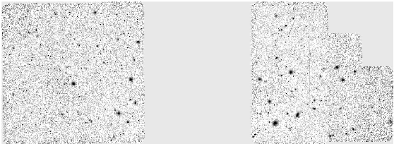
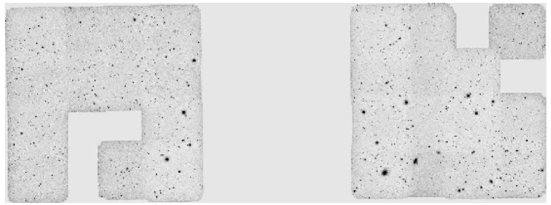
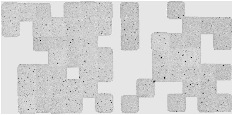
Figure 6: The coverage in the Deep1 region (north up, east left). From top to bottom it is $J$ ($51\aas@@fstack{\prime}8\times 19\aas@@fstack{\prime}0$), deep $K_{s}$ ($51\aas@@fstack{\prime}9\times 19\aas@@fstack{\prime}1$), and shallow $K_{s}$ ($64\aas@@fstack{\prime}3\times 31\aas@@fstack{\prime}5$). The two fields included are Deep1a (left) and Deep1b (right).

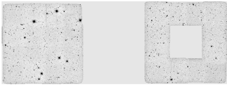
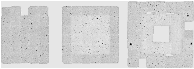
Figure 7: The coverage in the Deep2 region (north up, east left). The $J$ coverage ($52\aas@@fstack{\prime}5\times 19\aas@@fstack{\prime}3$) is on the top and $K_{s}$ ($90\aas@@fstack{\prime}8\times 31\aas@@fstack{\prime}2$) on the bottom. The fields in the upper panel are Deep2b (left) and Deep2c (right). The fields in the lower panel are Deep2a, Deep2b and Deep2c from left to right. In the $K_{s}$-band the central parts in $K_{s}$ for the mosaics Deep2b and Deep2c are the deep strategy, for Deep2a only shallow data exists.

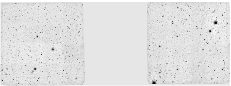
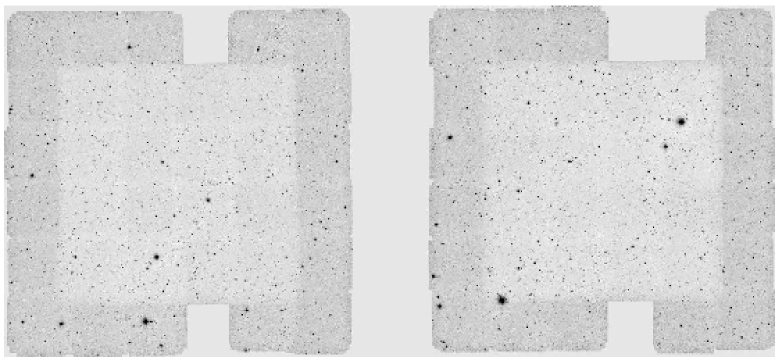
Figure 8: The coverage in the Deep3 region (north up, east left) with $J$ ($52\aas@@fstack{\prime}0\times 19\aas@@fstack{\prime}1$) on the top and $K_{s}$ ($60\aas@@fstack{\prime}1\times 27\aas@@fstack{\prime}3$) on the bottom. The fields are Deep3a (left) and Deep3b (right). For the $K_{s}$-band the central parts correspond to the deep strategy.

The completeness of the survey is measured not only in terms of depth but also in areal coverage. The latter can be assessed from Figs. 6-8, in the appendix. These figures show the final coverage for each region and strategy, after discarding images with grade D. Note that in the case of Deep1 the $K_{s}$ deep observations were done independently of those conducted for $K_{s}$-shallow. As can be seen the areal completeness and connectivity of the mosaics are high, with the exception of the shallow observations of Deep1a and b, which are 70% and 53% areal complete, respectively.

4.2 Source lists

Figure 1: Distribution of the 80% completeness limiting Vega-magnitudes for each of the three observing strategies as indicated in each panel.

Table 8: Summary of the properties of the catalogs extracted for each mosaic and band.

Field	Passband	#Catalogs	Eff. area	#Objects	80% compl.
Deep1a	$J$	16	29.4$\pm$ 1.0	908$\pm$ 110	21.50$\pm$ 0.23
Deep1b	$J$	13	28.7$\pm$ 1.8	665$\pm$ 145	21.57$\pm$ 0.51
Deep2b	$J$	16	29.4$\pm$ 1.0	828$\pm$ 90	21.48$\pm$ 0.23
Deep2c	$J$	12	28.8$\pm$ 2.1	811$\pm$ 208	21.41$\pm$ 0.25
Deep3a	$J$	16	27.2$\pm$ 2.2	934$\pm$ 178	21.52$\pm$ 0.38
Deep3b	$J$	16	29.4$\pm$ 0.7	907$\pm$ 80	21.44$\pm$ 0.25
Shallow
Deep1a	$K_{s}$	35	26.0$\pm$ 1.1	361$\pm$ 161	18.94$\pm$ 0.38
Deep1b	$K_{s}$	26	24.6$\pm$ 1.7	484$\pm$ 112	18.95$\pm$ 0.24
Deep2a	$K_{s}$	29	26.1$\pm$ 1.6	440$\pm$ 91	19.05$\pm$ 0.22
Deep2b	$K_{s}$	20	26.1$\pm$ 1.2	479$\pm$ 78	19.05$\pm$ 0.17
Deep2c	$K_{s}$	34	25.7$\pm$ 1.6	318$\pm$ 188	18.79$\pm$ 0.47
Deep3a	$K_{s}$	18	26.3$\pm$ 0.5	593$\pm$ 98	19.01$\pm$ 0.09
Deep3b	$K_{s}$	17	26.7$\pm$ 0.6	551$\pm$ 53	18.91$\pm$ 0.08
Deep
Deep1a	$K_{s}$	13	29.4$\pm$ 1.1	996$\pm$ 133	19.40$\pm$ 0.22
Deep1b	$K_{s}$	14	28.9$\pm$ 1.2	660$\pm$ 117	19.57$\pm$ 0.48
Deep2b	$K_{s}$	16	28.1$\pm$ 0.8	697$\pm$ 61	19.70$\pm$ 0.21
Deep2c	$K_{s}$	12	28.6$\pm$ 1.7	699$\pm$ 80	19.52$\pm$ 0.21
Deep3a	$K_{s}$	16	26.9$\pm$ 1.9	804$\pm$ 126	19.63$\pm$ 0.18
Deep3b	$K_{s}$	16	29.8$\pm$ 0.6	932$\pm$ 161	19.63$\pm$ 0.12
* includes Deep

Catalogs were extracted from the stacked images using the EIS Data Reduction System adopting the same procedures as described in Papers I and II. A description of the catalog format is found in the appendices of Paper I. These catalogs include only objects with $S/N\geq 3$ as computed from the magnitude error. Table 8 summarizes some of the main characteristics of the extracted catalogs. The table gives in Col. 1 the field name, in Col. 2 the passband, in Col. 3 the average and standard deviation of the effective area in square arcmin, in Col. 4 the average and standard deviation of the number of objects, and in Col. 5 the average and standard deviation of the 80% completeness limit in the Vega system. These completeness limits are for extended objects (see Paper I for details). Their distribution for each strategy is illustrated in Fig. 1. There is a total of 89 $J$ and 87 $K_{s}$ catalogs with mean values of the 80% completeness magnitude of $21.49\pm 0.31$ and $19.57\pm 0.28$ mag in the Vega system, with each catalog covering an area of $\sim 28.8$ square arcmin. For the shallow $K_{s}$ strategy there are 179 images with a mean 80% completeness magnitude in the Vega system of $18.94\pm 0.31$ mag, with a typical coverage of $\sim 25.8$ square arcmin.

Inspection of the CLASS_STAR parameter as a function of magnitude indicates that stars and galaxies can be adequately classified by using CLASS_STAR with a threshold of 0.90 at magnitudes $K_{s}\leq 17.0$ in both the deep and shallow data sets. For the $J$-band we identify stars brighter than $J=18.0$. At fainter magnitudes we take all objects to be galaxies. In the next section, these catalogs are used to assess the scientific quality of the survey data.

5 Discussion

5.1 Internal photometric comparison

Table 9: Mean magnitude offsets and standard deviations for each mosaic

Field	Passband	# overlaps	Mag. offset	Std.dev.
Deep1a	$J$	24	-0.02	0.11
Deep1b	$J$	15	0.05	0.11
Deep2b	$J$	24	0.03	0.05
Deep2c	$J$	12	-0.03	0.08
Deep3a	$J$	24	-0.02	0.06
Deep3b	$J$	24	0.02	0.04
Shallow
Deep1a	$K_{s}$	36	0.07	0.13
Deep1b	$K_{s}$	21	0.02	0.18
Deep2a	$K_{s}$	39	0.08	0.12
Deep2b	$K_{s}$	8	0.06	0.22
Deep2c	$K_{s}$	34	0.05	0.13
Deep3a	$K_{s}$	15	0.06	0.08
Deep3b	$K_{s}$	14	0.01	0.10
Deep
Deep1a	$K_{s}$	14	0.00	0.10
Deep1b	$K_{s}$	16	0.03	0.11
Deep2b	$K_{s}$	24	0.03	0.09
Deep2c	$K_{s}$	12	0.00	0.08
Deep3a	$K_{s}$	19	0.03	0.07
Deep3b	$K_{s}$	24	0.05	0.08

The consistency of the photometric calibration of the individual pointings, and therefore of the mosaic, was assessed by comparing the magnitudes of objects in common between adjacent frames. For each mosaic the mean and standard deviation of the magnitude difference of all pairs of sources in common in adjacent frames were computed, considering only objects with a magnitude error $<0.2$ ($\sim 5\sigma$). Ideally, one would use only stars for this, but because the number of objects in the overlaps is small, it proved necessary to include galaxies as well. In Table 9 these mean offsets and standard deviations are listed for each mosaic. The table lists in Col. 1 the field name, in Col. 2 the passband, in Col. 3 the number of overlaps in the mosaic, in Cols. 4 and 5 the mean and standard deviation of the magnitude offsets. From the table one finds that on average the offsets are small, typically $\lesssim 0.05$ mag. The scatter is typically less than 0.1 mag. In all cases the mean offset is smaller than the standard deviation. Combined these results suggest a homogeneous photometric calibration across the mosaics with fairly small field-to-field variations.

In an attempt to improve the match among different zero points obtained on different nights, correct for data taken under non-photometric conditions, and hence minimize field-to-field variations, the method employed by Maddox et al. (1990) was utilized. Taking into account the computed corrections, one finds that, in general, the mean offsets do not change significantly and the scatter decreases only marginally. This result may be partly due to the large uncertainty in each individual offset caused by the small number of sources in the overlap regions and the necessity to include galaxies. However, it may also indicate a good match among the original zero points.

5.2 External comparison

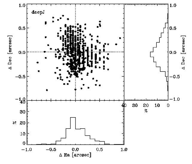
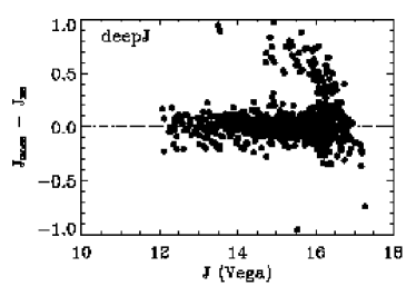
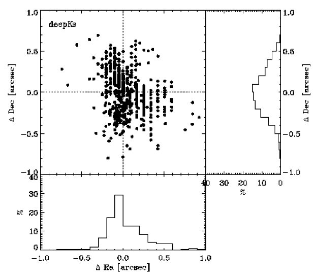
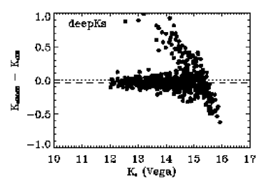
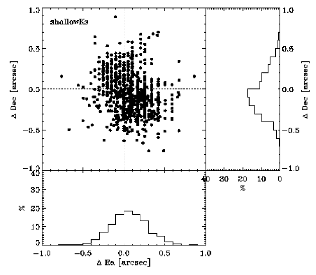
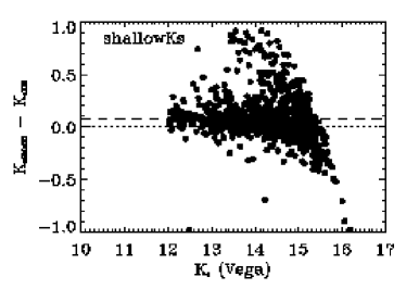
Figure 2: Astrometric (left column) and photometric (right column) comparison between objects in common between the EIS and 2MASS surveys. The offsets are computed as 2MASS $-$ EIS. The rows correspond to each adopted strategy as indicated. Dotted lines indicate the zero offset location, while the dashed lines in the right panels depict the mean offset computed for the bright objects as discussed in the text. In this plot magnitudes are in the Vega system.

In order to externally verify the survey products, the source lists extracted from the final images as described in the previous section were cross-correlated with the point source catalog available from the 2MASS survey (Skrutskie et al., 2006). This was carried out adopting a search radius of 1″. A total of 1056, 966, 1539 objects were found in common for the $J$, and the deep and shallow $K_{s}$ -band final images, respectively, over all regions covered by the survey. The differences in position and magnitude for objects in common and considered “good” in both catalogs (5$\sigma$ detections and in the case of 2MASS not contaminated by neighboring objects) were computed and their distribution as a function of right ascension and declination (left panels) and magnitude (right panels) are shown in Fig. 2. The mean offset in position is negligible and amounts to at most $\sim 0\aas@@fstack{\prime\prime}07$ for the shallow $K_{s}$ strategy. The scatter is of $0\aas@@fstack{\prime\prime}23$ and $0\aas@@fstack{\prime\prime}27$ in right ascension and declination, respectively, for all strategies. This is consistent with an astrometric accuracy of $\sim 0\aas@@fstack{\prime\prime}19$ for the EIS images, limited by the typical internal accuracy of the reference catalog used.

Considering objects brighter than $J=16.0$ and $K_{s}=14.5$ (Vega system) the measured magnitudes of the two data sets are in good agreement. At fainter magnitudes the scatter increases and the effects of the Malmquist bias introduced by the depth of the 2MASS data are seen. Objects with magnitudes brighter than 12 mag are saturated in the EIS data and therefore discarded from the plots. For the deep strategies the systematic offset in magnitude is (discarding the outlying objects with offsets in excess of 0.5 mag) $\sim-0.04$ mag with a scatter of 0.07 in $K_{s}$ and $\sim 0.0$ with a scatter of 0.08 in $J$, consistent with the estimated uncertainty of the overall zero-point (Sect. 3). For the shallow $K_{s}$ -survey one finds a mean offset of $\sim 0.08$ mag and a scatter of $\sim 0.13$ mag. The amplitude of the scatter is remarkably small, considering the values obtained in the previous section, and demonstrates the uniformity of the photometric calibration of the present data across the sky.

5.3 Comparison of galaxy and star counts

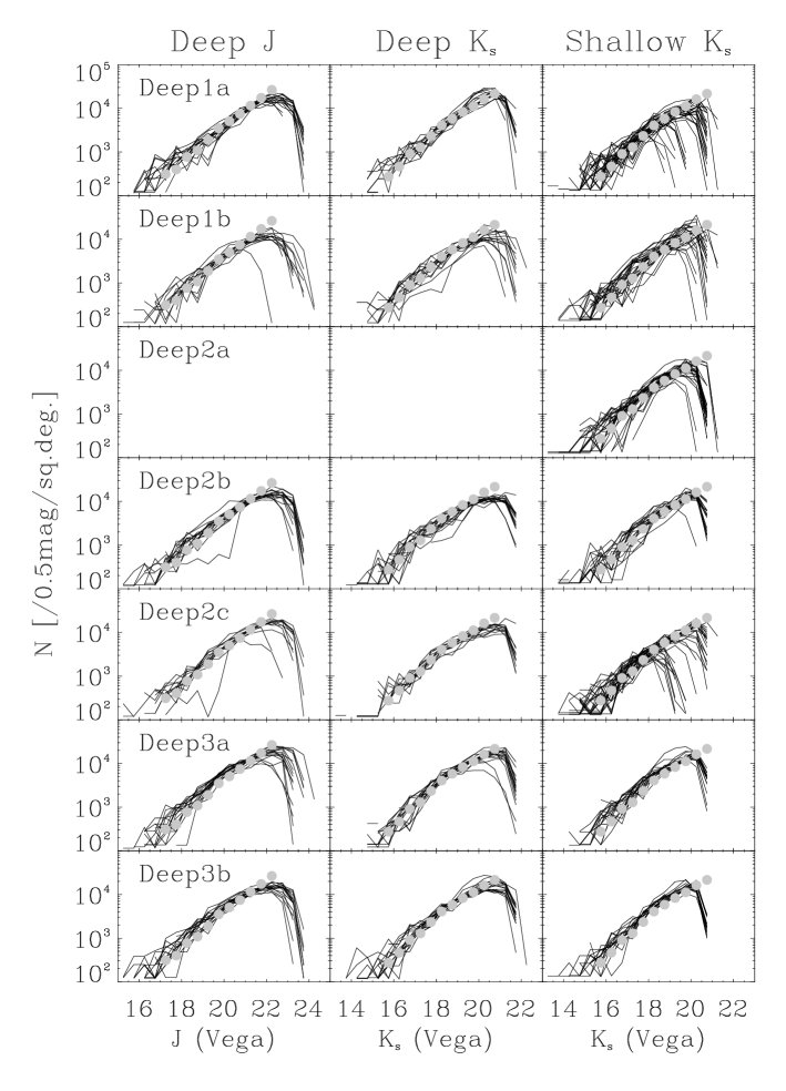
Figure 3: Galaxy counts for each individual pointing grouped by mosaic (lines) compared with those of Iovino et al. (2005, solid circles).

An alternative way to evaluate the data is to compare the counts of galaxies and stars with those computed by other authors and/or predicted by models. For galaxies this is illustrated in Fig. 3. The figure shows for each passband and strategy (columns) the galaxy counts obtained for each pointing (thin lines) grouped by mosaic (rows), as indicated in the panels of the leftmost panel of each row. These are compared with the counts recently reported by Iovino et al. (2005, solid circles). Here galaxies are 3$\sigma$ detections with CLASS_STAR$<0.9$. From the figure one can easily: 1) identify individual cases that depart significantly from the mean; 2) have a clear measure of the variance introduced from field-to-field variations due to the relatively small field of view of SOFI; and 3) identify the variation in depth of a few pointings, such as in the case of Deep1a $K_{s}$-shallow among others. Moreover, the relatively small scatter at intermediate magnitudes among the subfields forming a mosaic indicates that the relative photometry between them is reasonable, reinforcing the evidence mentioned above. More importantly, on average, there is an excellent agreement with the counts of Iovino et al. (2005), which reach a comparable depth to the deep $J$$K_{s}$ strategy. This can be seen in Fig. 4 which shows the average counts obtained taking into account all fields and regions for the $J$- and $K_{s}$-band data. In all cases each field contributes only at magnitudes brighter than their respective 80% completeness limit, and no completeness corrections have been attempted. These mean counts show an excellent agreement with those recently obtained by different authors (Väisänen et al., 2000; Martini, 2001; Iovino et al., 2005), being further strong evidence of the overall quality of the data. The mean counts for the $J$- and $K_{s}$-bands are given in Tables 10 and 11 listing in Col. 1 the center of the magnitude bin in the Vega system, in Col. 2 the number of galaxies per 0.5 mag and per square degree, and in Col. 3 the standard deviation among the contributing fields.

Figure 4: Comparison of galaxy number counts in the $J$- (top) and $K_{s}$-band (bottom) between the present work (solid circles with error bars); diamonds denote Väisänen et al. (2000), triangles Martini (2001) and squares Iovino et al. (2005).

Table 10: The derived raw galaxy counts for the $J$-band. The counts are given per mag per square degree. Each field only contributes to the bins brighter than their 80% completeness limit. No completeness correction has been attempted.

Mag	N	$\sigma_{N}$
10.25	0.0	0.0
10.75	0.0	0.0
11.25	0.0	0.0
11.75	0.0	0.0
12.25	2.9	26.9
12.75	2.8	26.0
13.25	2.8	26.0
13.75	10.9	50.8
14.25	11.2	52.2
14.75	47.4	110.8
15.25	73.7	135.3
15.75	93.7	156.4
16.25	283.3	255.6
16.75	444.5	381.0
17.25	766.0	463.1
17.75	1350.6	606.4
18.25	2059.3	746.3
18.75	3189.6	1083.7
19.25	4988.9	1731.7
19.75	7804.7	2398.9
20.25	11671.5	3354.3
20.75	16064.9	3381.6
21.25	18383.9	5991.3
21.75	12933.6	8897.6
22.25	10949.9	10678.0

Table 11: The derived raw galaxy counts for the $K_{s}$-band. The counts are given per mag per square degree. Each field only contributes to the bins brighter than their 80% completeness limit. No completeness correction has been attempted.

Mag	N	$\sigma_{N}$
11.25	0.9	14.6
11.75	4.1	33.6
12.25	2.1	24.2
12.75	11.9	54.9
13.25	20.2	77.1
13.75	51.8	118.7
14.25	121.2	209.2
14.75	224.4	254.5
15.25	471.6	421.6
15.75	747.9	509.5
16.25	1282.1	664.6
16.75	2144.8	932.2
17.25	3598.5	1366.0
17.75	5721.6	1832.1
18.25	8872.0	2904.3
18.75	11606.3	3772.5
19.25	10333.8	5998.6
19.75	8330.2	5731.2
20.25	5295.8	5289.0

Finally, the corresponding stellar counts, sources with CLASS_STAR$\geq 0.9$, are shown in Fig. 5. The counts (solid circles connected by a solid line) are compared to predictions adopting the model proposed by Girardi et al. (2005, thin lines). Despite the large scatter due to the small field-of-view, the agreement is remarkable, considering the different regions and that the model was parameterized using optical data.

Figure 5: Comparison of star counts (filled circles connected by solid line) for each mosaic (rows) and strategy (columns) compared with model predictions by Girardi et al. (2005, thin line).

6 Summary

This paper presents the infrared data accumulated by the Deep Public Survey conducted by the EIS program. The paper presents the observations, reductions, and some of the main products generated and administrated by the EIS Data Reduction System which allows the unsupervised reduction of large amounts of data. For instance, the data set described in the present paper was reduced overnight using eight dual-processors computers running Linux. The highthroughput of the system also makes it ideal for handling the new generation of infrared surveys using wide-field cameras. In general, the depth of the survey is relatively homogeneous and the coverage rather uniform with exception of the shallow coverage of Deep1. However, considerable improvement in coverage and photometric accuracy could have been reached if the survey was carried out in service rather than visitor mode allowing a better optimization depending on the actual weather conditions, in particular ensuring sufficient photometric data for reliable calibration of all the fields.

The near-infrared dataset being released is one of largest currently available and its quality has been assessed qualitatively by visual inspection of the individual images and quantitatively by direct comparison with measurements made by the 2MASS survey limited to the bright end and by the comparison of galaxy and star counts with those of other authors and with model predictions.

The depth and areal coverage in the near-infrared combined with the deep multi-wavelength optical data reported in Paper III make this data set extremely useful to further explore the nature of extremely red objects (e.g. Kong et al., 2006) and to search for distant galaxy clusters. With this paper, all the infrared data accumulated by the EIS project up to late 2004 are now in the public domain.

Appendix A Coverage per region

In this appendix, figures giving an overview of the final coverage for each mosaic are presented. Each figure covers one region (Deep1, Deep2 or Deep3). For Deep1 there are three figures ($J$, deep $K_{s}$, and shallow $K_{s}$), while for Deep2 and Deep3 only two figures ($J$ and $K_{s}$) are available since here the deep $K_{s}$ strategy fills the central parts of the shallow mosaics. The relative sizes among the fields reflect their relative sky-coverage.

From the figures it is clear that the areal completeness of the mosaics are in general high, even though the Deep1 shallow $K_{s}$ mosaics suffer from incompleteness, leading to large difficulties in creating mosaics and carrying out an internal re-calibration to establish a common magnitude system for all frames. The centers of each subfield can be found in Table 1.

References

- Cristiani et al. (2000) Cristiani, S., Appenzeller, I., Arnouts, S., et al. 2000, A&A, 359, 489
- da Costa et al. (1998) da Costa, L., Nonino, M., Rengelink, R., et al. 1998, astro-ph/9812105
- da Costa et al. (2004) da Costa, L., Rite, C., & Slijkhuis, R. G. 2004, in ASP Conf. Ser. 314: Astronomical Data Analysis Software and Systems (ADASS) XIII, 3
- Dickinson & Giavalisco (2003) Dickinson, M. & Giavalisco, M. 2003, in The Mass of Galaxies at Low and High Redshift, 324
- Dietrich et al. (2006) Dietrich, J. P., Miralles, J.-M., Olsen, L. F., et al. 2006, A&A, 449, 837, Paper I
- Djamdji et al. (1993) Djamdji, J., Bijaoui, A., & Manière, R. 1993, in Photogrammetric Engineering and Remote Sensing, Vol. 59, 645
- Elston et al. (2006) Elston, R. J., Gonzalez, A. H., McKenzie, E., et al. 2006, ApJ, 639, 816
- Giavalisco et al. (2004) Giavalisco, M., Ferguson, H. C., Koekemoer, A. M., et al. 2004, ApJ, 600, L93
- Girardi et al. (2005) Girardi, L., Groenewegen, M., Hatziminaoglou, E., & da Costa, L. 2005, A&A, 436, 895
- Iovino et al. (2005) Iovino, A., McCracken, H., Garilli, B., et al. 2005, A&A, 442, 423
- Kong et al. (2006) Kong, X., Daddi, E., Arimoto, N., et al. 2006, ApJ, 638, 72
- Maddox et al. (1990) Maddox, S. J., Efstathiou, G., & Sutherland, W. J. 1990, MNRAS, 246, 433
- Martini (2001) Martini, P. 2001, AJ, 121, 598
- Mignano et al. (2006) Mignano, A., Miralles, J.-M., da Costa, L., et al. 2006, submitted to A&A, Paper III
- Moorwood et al. (1998) Moorwood, A., Cuby, J., & Lidman, C. 1998, The Messenger, 91
- Olsen et al. (2006) Olsen, L. F., Miralles, J.-M., da Costa, L., et al. 2006, A&A, 452, 119, Paper II
- Persson et al. (1998) Persson, S., Murphy, D., Krzeminski, W., Roth, M., & Rieke, M. 1998, AJ, 116
- Rengelink et al. (1998) Rengelink, R., Nonino, M., da Costa, L., et al. 1998, astro-ph/9812190
- Skrutskie et al. (2006) Skrutskie, M. F., Cutri, R. M., Stiening, R., et al. 2006, AJ, 131, 1163
- Väisänen et al. (2000) Väisänen, P., Tollestrup, E., Willner, S., & Cohen, M. 2000, AJ, 540, 593