Sulphur abundances in disk stars as determined from the forbidden $\lambda 10821$ [S i] line

Abstract

Aims. In this paper we aim to study the chemical evolution of sulphur in the galactic disk, using a new optimal abundance indicator: the [S i] line at 10821 Å. Similar to the optimal oxygen indicators, the [O i] lines, the [S i] line has the virtues of being less sensitive to the assumed temperatures of the stars investigated and of likely being less prone to non-LTE effects than other tracers.

Methods. High-resolution, near-infrared spectra of the [S i] line are recorded using the Phoenix spectrometer on the Gemini South telescope. The analysis is based on 1D, LTE model atmospheres using a homogeneous set of stellar parameters.

Results. The $\lambda 10821$ [S i] line is suitable for an abundance analysis of disk stars, and the sulphur abundances derived from it are consistent with abundances derived from other tracers. We corroborate that, for disk stars, the trend of sulphur-to-iron ratios with metallicity is similar to that found for other alpha elements, supporting the idea of a common nucleosynthetic origin.

1 Introduction

To extract information about the nucleosynthesis of the $\alpha$ elements (e.g., Mg, Si, S, and Ca), accurate data on their abundances for stars in the galactic halo and disk are essential. Sulphur is one of the least studied $\alpha$ elements, owing to the paucity of appropriate spectral lines. The diagnostics tools used for sulphur so far are multiplets of transitions from highly excited levels, such as the $\lambda\lambda 6743-57$, $\lambda\lambda 8694-95$, and $\lambda\lambda 9213-38$ Å lines (corresponding to the oxygen triplet at 7775 Å). The derived abundances from these lines are sensitive to the adopted $T_{\mathrm{eff}}$ of the star and could be susceptible to non-LTE effects that are difficult to quantify owing to a lack of adequate atomic data. Thus, these multiplets may lead to uncertain sulphur abundances. A recent debate in the literature has questioned the origin of sulphur in the early universe, as well as whether sulphur follows the evolution of the other $\alpha$ elements or not, partly owing to these uncertainties, but also due to the weakness of lines used (see for example Israelian & Rebolo 2001; Takada-Hidai et al. 2002; Nissen et al. 2004; Ryde & Lambert 2004, 2005; Korn & Ryde 2005).

Sulphur and oxygen belong to the same group in the periodic table and have the same number of valence shell electrons, which means that their spectra show some similarities, and similar diagnostic lines are available for the determination of their elemental abundances in stars. In the same way as for the $\lambda 6300$ and $\lambda 6363$ Å [O i ] lines from the ground state, which have been extensively used and discussed for the determination of oxygen abundances in stars (see for example Asplund et al. 2004; Nissen et al. 2002; Garcia Pérez et al. 2006), the corresponding [S i] lines should not be susceptible to non-LTE effects, nor should they be very dependent on the adopted $T_{\mathrm{eff}}$. These virtues make it worthwhile to investigate the $\lambda 10821$ [S i] line as a spectroscopic tracer of stellar sulphur abundances. The reason why this line has not previously been used is that it lies beyond the reach for normal optical CCDs. The near-infrared region also has several other advantages for an abundance study of cool stars (Ryde et al. 2005).

In this Letter we present the first attempt to determine stellar sulphur abundances based on the forbidden sulphur line at 10821.18 Å (in air). This line is an inter-combination line, an M1 transition between the triplet ground-state (${}^{3}P_{2}$) and the first excited singlet state (${}^{1}D_{2}$). We explore its use in stars of the galactic disk since it is important to evaluate this new preferred diagnostic and to scrutinize the evolution of sulphur in the disk based on other diagnostics. The abundances of sulphur in disk stars have earlier been studied by Clegg et al. (1981), Francois (1987), Chen et al. (2002), and Caffau et al. (2005).

2 Observations

The [S i] line was observed at a high signal-to-noise ratio ($\mathrm{SNR}\approx 200$), in a sample of G and K subgiants and giants of the galactic disk. The homogeneous set of stars was selected from the library of F5-K7 stars observed with the Elodie spectrometer (Soubiran et al. 1998) and are listed in Table 1. Our high-resolution, near-infrared spectra were recorded with the Phoenix spectrometer mounted on the Gemini South telescope. Phoenix is a cryogenic, single order echelle spectrometer with an Aladdin $512\times 1024$ element InSb detector array cooled to 35 K (Hinkle et al. 1998). We used a 3 pixel wide slit resulting in a spectral resolution of $R\sim 60,000$. The spectra were centered on the $\lambda 10821$ [S i] line and covered the 9220-9260 cm^-1 region. The data were obtained in service observing mode (Programme ID: GS-2004A-Q-13) over a period from 5/4 2004 to 23/6 2005.

The data were processed in a standard manner with the reduction package IRAF (e.g., Tody 1993) to retrieve one-dimensional, continuum-normalized, and wavelength-calibrated stellar spectra. The raw images were trimmed and a normalized flat frame was made by dividing a master flat by a Legendre polynomial to fit the overall spectral shape in the dispersion direction. The observations were performed in pairs such that the star was moved approximately $5\arcsec$ along the slit between two equally long exposures. These two exposures were subsequently subtracted from each other, a process that reduces the sky background. A hot calibration star, recording telluric atmospheric absorption lines, was used partly for the wavelength calibration and partly to eliminate the telluric spectral contamination. The multiple exposures of the same star made it possible to apply a cosmic-ray-hit rejection algorithm when adding them together in the form of 1-dimensional spectra. Due to residual fringing, a high-order polynomial was used to rectify and normalize the spectra. An example of a spectrum, with lines identified, is shown in Fig. 1.

Figure 1: The spectrum of the star HD212943 is shown by dots. The full line shows a synthetic spectrum with $\mathrm{[S/Fe]}=0.21$, based on a model atmosphere with the following fundamental parameters: $T_{\mathrm{eff}}=4586$ K, $\log g=2.81$ (cgs), [Fe/H]$=-0.34$, $\xi_{\mathrm{micro}}=1.5\,\mathrm{km\,s^{-1}}$, and $\xi_{\mathrm{macro}}=4.5\,\mathrm{km\,s^{-1}}$.

In the analysis the equivalent width of the $\lambda 10821$ [S i] line was measured using the deblending algorithm in IRAF, since the wing of a Cr i line blends into the wing of the [S i] line. Gaussian fits were used, and we estimate the measuring uncertainty to be 10%, leading to an uncertainty in the derived sulphur abundance of the order of 0.03 dex, as estimated from individual measurements. The equivalent widths are given in Table 1.

3 Analysis

Table 1: The stars investigated. Columns 3-6 give the atmospheric parameters of the stars, after Soubiran et al. (1998). The two subsequent columns provide the dates and the exposure times of the observations of the stars. The last four columns give our measured equivalent widths of the $\lambda 10821$ [S i] line, the derived logarithmic number abundance of sulphur relative to hydrogen, the logarithmic sulphur abundance relative to the Sun, and finally, the logarithmic sulphur-to-metallicity ratio relative to the solar values. In the second part of the table the stellar parameters for two stars from Fuhrmann (2004), and the sulphur abundances we derive based on these, are presented. We have used a solar sulphur abundance of $\log\varepsilon_{\odot}(\mathrm{S})\equiv\log N_{\mathrm{S}}/N_{\mathrm{H}}+12=7.20$ (Chen et al., 2002).

$$\begin{array}[]{llcccccccccc}\hline\cr\hline\cr\vskip 3.0pt plus 1.0pt minus 1.0pt\cr\mathrm{Star}&\mathrm{Spectral}&T_{\mathrm{eff}}&\log(g)&\mathrm{[Fe/H]}&\xi_{\mathrm{micro}}/\xi_{\mathrm{macro}}&\mathrm{Date\,\,of}&\mathrm{Exposure\,\,time}&W_{\mathrm{S}}&\log\varepsilon(\mathrm{S})&\mathrm{[S/H]}&\mathrm{[S/Fe]}\\ &\mathrm{type}&\mathrm{[K]}&\mathrm{[cgs]}&&\mathrm{[km\,\,s^{-1}}]&\mathrm{observations}&\mathrm{[s}]&\mathrm{[m\AA]}&&\\ \hline\cr\vskip 3.0pt plus 1.0pt minus 1.0pt\cr\textrm{\object{HD~3546}}&\textrm{G5III}&4942&2.73&-0.66&1.5/5.5&\textrm{July 6, 2004}&120&11.8&6.79&-0.41&0.25\\ \textrm{\object{HD~10380}}&\textrm{K3III}&4057&1.43&-0.25&1.5/5.5&\textrm{July 6, 2004}&60&56.9&6.98&-0.22&0.03\\ \textrm{\object{HD~40460}}&\textrm{K1III}&4741&2.00&-0.50&1.5/5.0&\textrm{Dec. 19, 2004}&480&18.3&6.70&-0.50&0.00\\ \textrm{\object{HD~81192}}&\textrm{G7III}&4705&2.50&-0.62&1.5/5.5&\textrm{April 6, 2004}&512&12.7&6.73&-0.47&0.15\\ \textrm{\object{HD~117876}}&\textrm{G8III}&4782&2.25&-0.50&1.5/5.0&\textrm{April 5, 2004}&480&19.9&6.80&-0.40&0.10\\ \textrm{\object{HD~139195}}&\textrm{K0p}&4856&2.82&-0.04&1.5/5.5&\textrm{May 17, 2004}&88&13.0&7.02&-0.18&-0.14\\ \textrm{\object{HD~161074}}&\textrm{K4III}&3980&1.73&-0.27&1.5/6.0&\textrm{June 22/23, 2005}&960&60.9&7.13&-0.07&0.20\\ \textrm{\object{HD~168723}}&\textrm{K0III-IV}&4859&3.13&-0.19&1.5/4.7&\textrm{May 17, 2004}&20&12.4&7.15&-0.05&0.14\\ \textrm{\object{HD~184406}}&\textrm{K3III}&4520&2.41&+0.01&1.5/5.0&\textrm{Aug. 7, 2004}&120&25.1&7.15&-0.05&-0.06\\ \textrm{\object{HD~188512}}&\textrm{G8IVvar}&5041&3.04&-0.04&1.5/5.0&\textrm{July 5, 2004}&180&9.1&6.98&-0.22&-0.18\\ \textrm{\object{HD~212943}}&\textrm{K0III}&4586&2.81&-0.34&1.5/4.5&\textrm{June 29, 2004}&84&19.9&7.07&-0.13&0.21\\ \textrm{\object{HD~214567}}&\textrm{G8II}&5038&2.50&+0.03&1.5/5.5&\textrm{June 30, 2004}&288&19.7&7.15&-0.05&-0.08\\ \textrm{\object{HD~219615}}&\textrm{G7III}&4830&2.57&-0.42&1.5/6.0&\textrm{June 29, 2004}&64&19.6&7.02&-0.18&0.24\\ \textrm{\object{HD~220954}}&\textrm{K1III}&4664&2.37&-0.10&1.5/5.5&\textrm{June 29, 2004}&48&30.0&7.19&-0.01&0.09\\ \vskip 3.0pt plus 1.0pt minus 1.0pt\cr\hline\cr\vskip 3.0pt plus 1.0pt minus 1.0pt\cr\textrm{HD\leavevmode\nobreak\ 168723}&\textrm{K0III-IV}&4921&2.99&-0.21&1.09/4.7&\textrm{May 17, 2004}&20&12.4&7.07&-0.13&0.08\\ \textrm{HD\leavevmode\nobreak\ 188512}&\textrm{G8IVvar}&5110&3.60&-0.17&0.92/5.0&\textrm{July 5, 2004}&180&9.1&7.23&+0.03&+0.20\\ \hline\cr\end{array}$$

For the analysis of the stellar spectra, 1D Marcs model atmospheres (Gustafsson et al., in preparation) are computed for each star. Sulphur abundances were derived from the equivalent widths, using the Eqwi code, and the synthetic spectra were calculated with the Bsyn code. Both codes use many subroutines from the Marcs code and solve the radiative transfer at many frequencies in each spectral line using the continuous opacity from the model atmosphere and the line opacity calculated from line lists. The fundamental stellar parameters of the observed stars, which are needed in the calculation of the stellar atmospheres, are taken from Soubiran et al. (1998) and are also given in Table 1. Moreover, a microturbulence of $1.5\,$km s^-1 is used and the usual linearly increased (for decreasing metallicity) $\alpha$ element enhancement for disk stars is assumed. The Marcs models used are hydrostatic model photospheres in spherical geometry (although not really necessary for the stars investigated here) and are computed assuming LTE, chemical equilibrium, homogeneity, and the conservation of the total flux (radiative plus convective, the convective flux being computed using the mixing length recipe). The radiation field used in the model generation is calculated with absorption from atoms and molecules by opacity sampling at approximately 95 000 wavelength points over the wavelength range $1300\,\mbox{\AA}$–$20\,\mbox{$\mu$m}$. The atomic opacity sampling files are calculated for metallicities of [Fe/H]$=0.0$, $-0.1$, $-0.25$, $-0.37$, $-0.5$, and $-0.75$, and the one closest in metallicity is used.

Molecular lines are included, but only CN (line list from Jørgensen & Larsson 1990, and Plez 1998, private communications) is important for the most metal-rich stars with low effective temperatures. TiO is, for example, unimportant even for the coolest of the stars. Atomic line data are taken from the VALD database (Piskunov et al. 1995) with the exception of the transition probability of the [S i] line, which is taken from the NIST database version 3 (see, e.g., Martin et al. 2000). The wavelength and strength of the Fe i line and the position of the two Cr i lines in the vicinity of the [S i] line are matched to fit the solar lines (see Table 2). To take additional line broadening into account, the synthetic spectra are convolved with a radial-tangential function (Gray 1992) with a macroturbulent velocity given in Table 1 as $\xi_{\mathrm{macro}}$. The synthetic spectra are used to inspect the location of the continuum, the line strengths and widths, and line blendings. For the stars we are investigating, no weak atomic blends are found at the [S i] line. The sulphur abundances are given in Table 1.

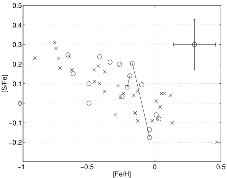
Figure 2: [S/Fe] vs. [Fe/H] plot for the stars investigated in this paper using the $\lambda 10821$ [S i] line (circles) and for the Chen et al. (2002) stars (crosses). Typical error bars are indicated. Squares indicate new sulphur abundances derived from a different set of stellar parameters for $\eta$ Ser and $\beta$ Aql (see text).

In Fig. 2 we have plotted our derived values of [S/Fe] vs. [Fe/H], as well as the the relative sulphur abundances derived for disk stars by Chen et al. (2002), who used optical, high-excitation S i lines ($\chi_{\mathrm{exc}}=7.9$ eV).

4 Discussion

We have chosen to use the stars in the library of Soubiran et al. (1998) to keep to a set of stars with homogeneously determined stellar parameters. The accuracies of the parameters given in Katz et al. (1998) for the stars in this library are $\delta T_{\mathrm{eff}}=86\,\mathrm{K}$, $\delta\log g=0.28\,\mathrm{dex}$, and $\delta\mathrm{[Fe/H]}=0.16\,\mathrm{dex}$. In Table 3 the uncertainties in the derived sulphur abundances due to uncertainties in the fundamental stellar parameters are shown. We also show the corresponding changes for the nearby Cr i and Fe i lines. Including the statistical measurement uncertainties, as estimated from the continuum placement and the effect of the SNR (both max 10% in $W_{\mathrm{S}}$), a conservative total uncertainty in the derived sulphur abundances is estimated to be $0.13\,\mathrm{dex}$. The uncertainty in the metallicity is taken from Katz et al. (1998), i.e., $\delta\mathrm{[Fe/H]}=0.16$ dex.

The strengths of weak lines depend on the line and continuum opacities, $\chi_{\mathrm{line}}$ and $\chi_{\mathrm{cont}}$, such that the equivalent width of a line $W\propto\chi_{\mathrm{line}}/\chi_{\mathrm{cont}}$. Since sulphur is mainly in the atomic state throughout the photospheres and since the weak [S i] line originates in the ground state, the sulphur line opacity (or the number of sulphur atoms in the ground state) is not very temperature sensitive. The continuous opacity of the wavelength region (H${}^{-}_{\mathrm{bf}}$) is slightly $T$-sensitive, but we see from Table 3 that the sulphur abundance derived is not very $T$-sensitive. Nor is the sulphur line opacity very sensitive to the electron pressure, although the continuous opacity is. This explains the sensitivity of the abundance derived from the observed equivalent width to the metallicity and especially to the surface gravity, as seen in Table 3. The Cr and Fe lines behave differently since they are from excited states, and (like H^-) represent a minority species in the photosphere. Therefore, the derived Cr and Fe abundances are more temperature sensitive, but are not as sensitive to the electron pressure. It can also be noted that the [S i] line is not saturated, and therefore not sensitive to $\xi_{\mathrm{micro}}$.

In the discussion on errors we have ignored systematic errors due to the treatment of convection in the atmospheres. A more proper way of treating convection is through ab initio 3D hydrodynamic models as described in, e.g., Asplund et al. (2000). For the [O i] lines, Nissen et al. (2002) show that for disk metallicities the 3D effects are less than 0.1 dex (decreasing with increasing metallicity) for their coolest dwarf (5800 K). The main effect is the change in the continuous opacity and not a change in the line opacity due to cooler upper layers. Sulphur is expected to behave in a similar fashion. The effect is unknown for giants and subgiants, and we did not include it in the present analysis.

In his careful analysis of nearby disk and halo stars, Fuhrmann (2004) has two stars in common with our star list, namely $\eta$ Ser (HD168723) and $\beta$ Aql (HD188512). The stellar parameters derived by him, and the alternative sulphur abundances derived by us using his stellar parameters, are also given in Table 1. As we saw in our uncertainty analysis, the most sensitive fundamental parameter of the stellar models influencing the abundance derived from the [S i] line is the surface gravity. In particular, the alternative surface gravity of HD188512 ($\log g=3.04\rightarrow 3.60$) is the major cause of the large change in the sulphur abundance of that star ($\log\varepsilon(\mathrm{S})=6.98\rightarrow 7.23$). Since the metallicity of HD188512 is also different ([Fe/H]$-0.04\rightarrow-0.17$), the position of the star in Fig. 2 changes quite dramatically. This again gives an indication of the uncertainties due to the stellar parameters only.

From Fig. 2 we see that the agreement with the abundance determination of Chen et al. (2002) is good given the level of uncertainties. Chen et al. (2002) showed that their S abundances correlated strongly with their Si abundances, the latter being a well studied $\alpha$ element, suggesting that the nucleosynthesis of sulphur is similar to that of the other $\alpha$ elements. We can thus corroborate that sulphur shows an evolution typical of an $\alpha$ element, and we have shown that the $\lambda 10821$ [S i] line is indeed a good diagnostic tool for the sulphur abundance in disk stars. The virtues of the line are that it is not very sensitive to $T_{\mathrm{eff}}$ and that it should not be subject to non-LTE effects. It is apparent that an uncertainty in the surface gravity affects the abundance derived from this line. It should, however, be noted that the [S/Fe] ratio will be much less dependant on gravity if the iron abundance is determined from Fe ii lines that react similarly to a change in electron pressure as the [S i] line. The question whether the $\lambda 10821$ [S i] line can also be used for stars of the galactic halo will be addressed in a forthcoming paper.

Table 2: Atomic line parameters. After the excitation energy, $\chi_{\mathrm{exc}}$, of the lower level of the transition, which is given in eV, the transition probability of the line as the logarithm of the product of the statistical weight and the oscillator strength is given.

$$\begin{array}[]{lcccc}\hline\cr\hline\cr\vskip 3.0pt plus 1.0pt minus 1.0pt\cr\mathrm{Element}&\mathrm{Wavenumber}&\mathrm{Wavelength}&\textrm{$\chi_{\mathrm{exc}}$}&\textrm{$\log\,gf$}\\ \vskip 3.0pt plus 1.0pt minus 1.0pt\cr&&\mathrm{(in\,\,vacuum)}\\ \vskip 3.0pt plus 1.0pt minus 1.0pt\cr&\textrm{[cm${}^{-1}$]}&\textrm{[\AA]}&\textrm{[eV]}&\\ \vskip 3.0pt plus 1.0pt minus 1.0pt\cr\hline\cr\vskip 3.0pt plus 1.0pt minus 1.0pt\cr\textrm{Cr \sc{i}}&9242.264&10819.860&3.013&-1.957\\ \textrm{Fe \sc{i}}&9241.082&10821.244&3.960&-2.178\\ \textrm{[S \sc{i}]}&9238.609&10824.140&0.000&-8.617\\ \textrm{Cr \sc{i}}&9238.200&10824.619&3.013&-1.678\\ \vskip 3.0pt plus 1.0pt minus 1.0pt\cr\hline\cr\vskip 3.0pt plus 1.0pt minus 1.0pt\cr\end{array}$$

Table 3: A representative example of the effects on logarithmic abundances derived for the S, Cr, and Fe lines in the observed wavelength region when the fundamental parameters of the model atmosphere of HD117876 are changed.

Uncertainty $$\mathrm{\Delta\log\varepsilon(S)}$$