On Dissipation inside Turbulent Convection Zones from 3D Simulations of Solar Convection

Abstract

The development of 2D and 3D simulations of solar convection has lead to a picture of convection quite unlike the usually assumed Kolmogorov spectrum turbulent flow. We investigate the impact of this changed structure on the dissipation properties of the convection zone, parametrized by an effective viscosity coefficient. We use an expansion treatment developed by Goodman & Oh 1997, applied to a numerical model of solar convection (Robinson et al. 2003) to calculate an effective viscosity as a function of frequency and compare this to currently existing prescriptions based on the assumption of Kolmogorov turbulence (Zahn 1966, Goldreich & Keeley 1977). The results match quite closely a linear scaling with period, even though this same formalism applied to a Kolmogorov spectrum of eddies gives a scaling with power-law index of $5\over 3$.

Turbulent (eddy) viscosity is often considered to be the main mechanism responsible for dissipation of tides and oscillations in convection zones of cool stars and planets (Goodman & Oh 1997, and references therein). Currently existing descriptions have been used, with varying success, to explain circularization cut-off periods for main sequence binary stars (Zahn & Bouchet 1989, Meibom & Mathieu 2005), the red edge of the Cepheid instability strip (Gonczi 1982) and damping of solar oscillations (Goldreich & Keeley 1977). However, this hypothesis has been far more successful in damping oscillations than damping tides, and different mechanisms have been proposed for the latter, especially for planets (see Wu 2004ab; Ogilvie & Lin 2004, and references therein). In this paper we reconsider the problem of tidal dissipation in stellar convection zones of solar-type stars using the turbulent velocity field from a realistic 3D solar simulation.

The standard treatment is to assume a Kolmogorov spectrum in the convection zone and apply some prescription to model the effectiveness of eddies in dissipating the given perturbation. Two prescriptions have been proposed to describe the efficiency of eddies in dissipating perturbations with periods smaller than the eddy turnover time.

Firstly according to Zahn(1966, 1989), when the period of the perturbation(T) is shorter than the eddy turnover time ($\tau$) the dissipation efficiency is decreased because in half a period the eddy only completes $T\over 2\tau$ of its churn, and hence the dissipation (viscosity) should be inhibited by the same factor:

$$\nu=\nu_{max}\min\left[\left(T\over 2\tau\right),1\right]$$ (1)

Where $\nu_{max}$ is some constant which depends on the mixing length parameter. With this assumption large eddies dominate the dissipation. This prescription has been tested against tidal circularization times for binaries containing a giant star (Verbunt and Phinney 1996), and is in general agreement with observations.

Secondly, Goldreich & Nicholson (1989) and Goldreich & Keely (1977) argue that the viscosity should be severely suppressed for eddies with $\tau\gg T$, and hence the dissipation should be dominated by the largest eddies with turnover times less than $T/2\pi$. From Kolmogorov scaling the viscosity on a given time-scale is quadratic in the time-scale, or:

$$\nu=\nu_{max}\min\left[\left(T\over 2\pi\tau\right)^{2},1\right]$$ (2)

This description has been used successfully by Goldreich & Keely (1977), Goldreich & Kumar(1988), Goldreich, Kumar & Murray (1994) to develop a theory for the damping of the solar $p$-modes. If the more effective dissipation was applied instead, severe changes would be required in the excitation mechanism in order to explain the observed $p$ mode amplitudes. However, this inefficient dissipation is inconsistent with observed tidal circularization for binary stars (Meibom & Mathieu 2005). Additionally, Gonczi (1982) argues that for pulsating stars the location of the red edge of the instability strip is more consistent with Zahn’s description of eddy viscosity than with that of Goldreich and collaborators.

However, Goodman & Oh (1997) gave a consistent hydrostatic derivation of the convective viscosity, using a perturbational approach. For a Kolmogorov scaling they obtained a result that is closer to the less efficient Goldreich & Nicholson viscosity than it is to Zahn’s. While providing a more sound theoretical basis for the former scaling, this does not resolve the observational problem of insufficient tidal dissipation.

Both 2D and 3D numerical simulations of the solar convection zone have revealed that the picture of a Kolmogorov spectrum of eddies is too simplified (Stein & Nordlund 1989, Robinson et al. 2003). The simulations showed that convection proceeds in a rather different, highly asymmetric fashion. This suggests that the problem of insufficient dissipation may be resolved by replacing the assumption of Kolmogorov turbulence with the velocity field produced from numerical simulations. More importantly, an asymmetric and non-Kolmogorov turbulence might dissipate different perturbations differently, i.e. depending both on the frequency and geometry of the perturbation. Such simulations have been used to develop a better model for the excitation of solar $p$-modes (Samadi et al. 2003).

Our approach is to apply the Goodman & Oh (1997) formalism to the velocity field obtained from realistic 3D solar surface convection in a small box. The 3D simulation was able to reproduce the frequency spectrum of solar $p$-modes. The main result is that we find a scaling relation with frequency that is in better agreement with the more efficient scaling proposed by Zahn, albeit for different reasons.

1 Method

We apply the Goodman & Oh (1997) treatment of convection to the velocity field of a 3D simulation of the outer layers of the sun. Goodman & Oh assume that a steady state convection zone velocity field ($\mathbf{v}$) is perturbed by introducing an external velocity ($\mathbf{V}$). They also assume that the convection occurs on scales small compared to the perturbation, and further that the convection is approximately incompressible and isentropic. Assuming that the convective length scales are small compared to the perturbation allowed them to consider a volume small enough to accommodate all convective scales, but over that volume the perturbation velocity field can be assumed linear in the Cartesian coordinates ($\mathbf{x}$):

$$\mathbf{V}=\mathbf{A}(t)\cdot\mathbf{x}$$ (3)

In other words we define the matrix $\mathbf{A}$ as the derivative matrix of $\mathbf{V}$:

$$A_{i,j}=\frac{\partial\mathbf{V}_{i}}{\partial x^{j}}$$

And keep only the first term in the Taylor series of $\mathbf{V}$.

Under this assumption means the results will only be applicable to perturbations that are large compared to the size of the simulation domain. In particular this prevents us from making any statements about the 5 minute solar oscillations, because the penetration depth of those is less than the box we use, and the coarse resolution prevent us from looking at only the upper part of the box.

Assuming incompressible and isentropic convection allows one to use the Eulerian equations for fluid motion:

$$\partial_{t}\mathbf{v}+\mathbf{V}\cdot\nabla\mathbf{v}+\mathbf{v}\cdot\nabla\mathbf{V}+\mathbf{v}\cdot\nabla\mathbf{v}+\nabla w=0$$ (4)

$$\nabla\cdot\mathbf{v}=0,$$ (5)

where $\nabla w$ incorporates pressure and gravitational acceleration, assumed to be gradients of scalar fields.

The problem has two dimensionless parameters: the tidal strain $\Omega^{-1}\left|\mathbf{A}\right|$, and $\left(\Omega\tau_{c}\right)^{-1}$, where $\Omega$ is the frequency of the perturbation and $\tau_{c}\equiv\frac{L_{c}}{V_{c}}$. The characteristic convective length scale is $L_{c}$ and $V_{c}$ is the characteristic convective velocity. In the case of hierarchical eddie structured convection $\tau_{c}$ is the eddy turnover time.

So using eq. 4 and eq. 5 one can express the perturbation in the convection velocity field in a coordinate system moving with the perturbation. Expanding in powers of the above dimensionless parameters and keeping only first order terms gives:

$$\delta_{1,1}\mathbf{v^{\prime}}(\mathbf{k},\omega)=-\frac{i}{\omega}\mathbf{P_{k}}\cdot\left[\mathbf{A}(\Omega)\cdot\mathbf{v}_{0}(\omega-\Omega,\mathbf{k})+\mathbf{A}(-\Omega)\cdot\mathbf{v}_{0}(\omega+\Omega),\mathbf{k})\right]$$ (6)

The subscripts of $\delta_{1,1}\mathbf{v^{\prime}}(\mathbf{k},\omega)$ indicate that only first order terms in the dimensionless parameters have been included, primes indicate quantities expressed in a coordinate system moving with the perturbation, and $\mathbf{v}_{0}$ is the convective velocity field in the absence of the perturbation. All of the above quantities are in Fourier space, because there the incompressibility is simply imposed by the projection operator:

$$\mathbf{P_{k}}\equiv\mathbf{I}-\frac{\mathbf{kk}}{k^{2}}$$

Eq. 6 can then be used to express the energy dissipation rate again as a power series in the two dimensionless quantities. Goodman and Oh s’ treatment implicitly assumes the box is small enough for the density not to vary significantly, and so it is sufficient to write the energy per unit mass as $\left<\mathbf{v}\cdot\mathbf{v}\right>$ and assume that to be independent of position.

In our case the simulation encompasses about 8 pressure scale heights so that the density varies significantly between the top and bottom. This means we need to use the dissipation per unit volume - $\left<\rho\mathbf{v}\cdot\mathbf{v}\right>$ - instead.

In order to avoid taking a 7 dimensional integral, which would be prohibitive in terms of computation time, we replace the density with its horizontal and temporal average leaving only the most important vertical dimension. Taking the time derivative of the energy per unit volume using that density and the perturbed convective velocity, our expression for the rate of dissipation per unit volume to lowest order becomes:

$$\dot{\mathcal{E}}_{2,2}=\mathbf{Re}\Bigg{\{}\int\frac{d^{3}\mathbf{k}\;dk^{\prime}_{z}}{(2\pi)^{4}}\rho^{*}(k_{z}+k^{\prime}_{z})\Big{[}\left<\mathbf{v}_{0}(\mathbf{k},-\Omega)\cdot\mathbf{A}(\Omega)\cdot\mathbf{P_{k^{\prime}}}\cdot\mathbf{A}(\Omega)\mathbf{v}_{0}(\mathbf{k^{\prime}},-\Omega)\right>$$

$$+\left.\mathbf{v}_{0}(\mathbf{k},-\Omega)\cdot\mathbf{A}(\Omega)\cdot\mathbf{P_{k^{\prime}}}\cdot\mathbf{A}(-\Omega)\mathbf{v}_{0}(\mathbf{k^{\prime}},\Omega)\right>\Big{]}\Bigg{\}}$$ (7)

Where $k^{\prime}=(-k_{x},-k_{y},k^{\prime}_{z})$, and the subscripts, as before, denote the order in the two dimensionless parameters characterizing the tide and the convection respectively. $\rho(k_{z})$ is the fourier transform of the density averaged over $x,y,t$. The normalization is such that $\rho(0)$ is the average density over all space and time.

Eq. 7 gives an anisotropic viscosity, for which we can obtain the different components by setting all terms of $\mathbf{A}$ to $0$ except for one, and comparing to the equivalent expression for the molecular viscosity:

$$\dot{\mathcal{E}}_{visc}=\frac{1}{2}\left<\rho\nu\right>\;Trace\left[\mathbf{A}(\Omega)\cdot\mathbf{A^{*}}(\Omega)\right]$$ (8)

Where the average is over the volume and over time.

2 Realistic 3D solar surface convection

The 3D simulation of the Sun is case D in Robinson et al. (2003). This has dimensions 2700 km $\times$ 2700 km $\times$ 2800 km on a $58\times 58\times 170$ grid. A detailed one-dimensional (1D) evolutionary model e.g. see Guenther et al. (1992) provided the starting model for the 3D simulation. Full details of the numerical approach and physical assumptions are described in Robinson et al. (2003).

The simulation extended from a few hundred km above the photosphere down to a depth of about 2500 km below the visible surface (photosphere). This is about 8 pressure scale heights. The box had periodic side walls and impenetrable top and bottom surfaces with a constant energy flux fed into the base and a conducting top boundary. The flux was computed from the 1D stellar model, thus was not arbitrary, but was the correct amount of energy flux the computation domain should transport outward in a particular star.

To get a thermally relaxed system in a reasonable amount of computer time, they used an implicit numerical scheme, ADISM (Alternating Direction Implicit on a Staggered Mesh) developed by Chan & Wolff (1982). Careful attention was paid to the geometric size of the box. Importantly the domain was deep enough and wide enough to ensure the boundaries had minimal effect on the bulk of the overturning convective eddies (or on the flow statistics). The convection simulation was run using the ADISM code until it reached a statistically steady state. This was checked by confirming that the influx and outflux of the box were within 5 % of each other and the run of the maximum velocity have reached an asymptotic state.

After the model was relaxed they sampled the entire 3D velocity field at 1 minute intervals. The data set used in this paper consists of 150 minutes of such solar surface convection. This is about 20 granule turnover life times. An example velocity snapshot of the convective flow is presented in fig. 1.

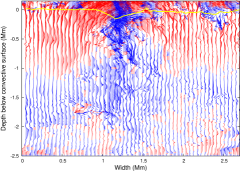
Figure 1: A sample snapshot of the convective flow. Blue color indicates downwarad flow, red indicates upward flow. The arrows show the velocity normalized to the sound speed. The yellow line represents the convective surface (i.e. where the entropy gradient is 0).

3 Results

We implement eqs. 7 and 8 by taking discrete Fourier transforms (FFT) of the velocity field and the averaging density horizontally and over time. In doing so it is important to verify that the windows introduced by the limited time and space extent of the simulation box do not dominate the results. This was done by repeating the calculation with the raw results, without any windowing and with Welch and Bartlett windows applied to all the dimensions simultaneously. As expected this has little or no effect on the frequency scaling (see below).

Figure 2: a) The off diagonal terms of the viscosity tensor compared to the z-z component. b) The diagonal terms of the viscosity tensor. c) The z-z component of the viscosity tensor (solid line) computed using eq. 7 and eq. 8 compared to the frequency scalings proposed by Zahn, Goldreich et. al. and Goodman and Oh. The horisontal axis for all the plots is the frequency in cycles per min.

As the viscosity tensor defined by eqs. 7 and 8 is clearly symmetric, it only contains 6 independent real valued components. Figure 2 displays the values of the viscosities we calculated.

Fig. 2a shows that the off diagonal terms are completely insignificant compared to the diagonal terms. Since in all the situations that concern us, the divergence of the perturbation field is never small compared to the other derivatives of the perturbing velocity field, the dissipation will be dominated by the diagonal terms. Hence their scaling with frequency will determine how the dissipation scales.

Fig. 2b shows that all the diagonal components scale roughly the same way with frequency and are dominated by the z-z component, although not by that dramatic a difference. Furthermore, for perturbations like tides the z derivative of the z component of the perturbation velocity is the largest element of the matrix $\mathbf{A}$ and hence that will be the term that will determine the frequency scaling of the dissipation.

In Fig. 2c we see the comparison between the different scalings with frequency suggested so far. We also show the scaling that we obtain by applying the Goodman and Oh (1997) method to a simulated 3D convection velocity field. The lines shown are least square fits to the curve we obtain from the simulation velocities. They seem to all intersect at the upper right-hand corner because the fits were done in linear space, not logarithmic, and hence do not tolerate even small deviations in the upper portion of the log-log plot. The best fit slope for our curve (not shown) is:

$$\nu\propto\Omega^{1.1\pm 0.1}$$

regardless whether we do the fit in linear or logarithmic space.

What are the possible sources of error in this result? Firstly we have assumed an incompressible flow in order to simplify the treatment. However, the fluid simulations used are not incompressible, because at the top of the convection zone, where most of the driving of the convection occurs, the flow velocities reach very close to the speed of sound and hence the flow is necessarily compressible. However, even though that layer is extremely important for the flow established below, it only contributes insignifficantly to the turbullent dissipation, because it only contains a few percent of the total mass. To verify that only a small fraction mass lies in a compressible region for each grid point, we define a compressibility parameter $\xi\equiv\tau_{c}\left|\nabla\cdot\mathbf{v}\right|$, where $\tau_{c}$ is the eddy turnover time in our box. In fig. 3 we plot the mass fraction with $\xi$ less than certain value. It is clear that the incompressibility assumption is violated only for a negligible fraction of the mass. As we noted before the flow is compressible only near the top of the box. To confirm that the presence of this region does not signifficantly affect our results we repeated the analysis separately for the top and bottom halves of the simulation box. The two new scalings obtained this way were completely consistent with the scaling of viscosity with frequency for the entire box.

Figure 3: The fraction of the total mass residing in a region with compressibility parameter $\xi\equiv\tau_{c}\nabla\cdot\mathbf{v}$ less than the given value.

Next, the fact that we have a finite (small) portion of the convection zone, both in time and in space could be important. We only treat the top portion of the solar convection zone and hope that the result is not very sensitive to depth. Of course it would be ideal to have the entire depth of the convection zone covered, but with current computational resources this is way outside of reach.

The finite span of the simulations may also be introducing edge effects which can be treated by applying some sort of a window function. We tried Welch, Bartlett and square window (no window). To verify that the time window available is large enough, we tried ignoring the last approximately $1/3$ of the data. We carried all those test on two independent runs of the model. The slopes this produced ranged from $\nu\propto\Omega^{0.98}$ to $\nu\propto\Omega^{1.19}$, where most of the difference originated from the two independent runs.

In addition the finite resolution might be leading to aliasing that could change our result. In particular make it flatter than it really is, by basically dumping additional power to the frequencies for which the dissipation is smallest (the places with higher value of the dissipation are less likely to be affected significantly). The effects of this can be seen in the diagonal viscosity components. The tails of their curves become flatter toward the end. The fact that this is restricted to the end of the curves is encouraging as it suggests only the high frequency end of the curve is affected. Also we have looked at crossections of the Fourier transformed velocity field and they do tail off at high $|k|$, which gives us confidence that the resolution is sufficient to capture most of the spectral power and that aliasing effects will be small.

Finally there are statistical errors associated with every point. Those can be estimated by noting the difference between $\nu_{xx}$ and $\nu_{yy}$ in Fig. 2b. Physically one expects that there should be no differences between the two horizontal directions of the simulation box, so the differences between them is some sort of measure of the error. In particular from there one can see that the first few points (at the low frequency end) are significantly less reliable than the rest, but apart from the first few points those errors become small. The average fractional uncertainty is $\sim 3\%$, which leads to an overall error in the slope of $0.01$.

Abandoning the Kolmogorov picture of turbullence clearly has a large effect on the result. Even though we use the approach of Goodman & Oh, which gives a power law index of $5/3$ for a Kolmogorov turbulence, our results give a scaling, rather different from the previous prescriptions. We also find that the viscosity is no longer isotropic. This is due to the signifficant difference in scaling between the velocity power spectrum with frequency and wavenumber in our simulation and the Kolmogorov prescription (see fig. 4). There are two important distictions apparent. First the frequency spectrum of our box is much shallower than the Kolmogorov prescription. This is responsible for the slower loss of efficiency of viscosity with frequency that we observe. Second the radial direction is clearly very different from the two horizontal directions — $v_{x}$ and $v_{y}$behave very differently from $v_{z}$ and the dependence of $\mathbf{v}$ on $x$ and $y$ is different from the $z$ dependence (fig. 4 a, b) — of course this results in the anisotropy of the viscosity tensor we calculate. Even though the spatial dependence of the horizontal velocity components is much different from the radial velocity spatial dependence, the frequency power spectrum of all three components scales roughly like $P\propto\Omega^{-1}$ (fig. 4c). From eq. 7 we see that if all the components of $\mathbf{v}$ have the same scaling with frequency, that same scaling will also apply for the viscosity, which is indeed what we observe.

Figure 4: a) Spatial power spectrum of the horizontal velocities. Only one of the horizontal componenents is plotted but the power spectrum of the other horizontal component is identical. b) Spatial power spectrum of the radial velocity. c) Frequency power spectrum of the three velocity components. The straight solid line - $P\propto\omega^{-1}$ - gives a good approximation to all three scalings.

4 Discussion

Our result is somewhat unexpected. It apparently stems from the fact that the structure of the convection velocity field produced by the 3D simulations is very different from simple isotropic Kolmogorov turbulence. The picture that emerges from these simulations consists of large scale slow up-flows penetrated by relatively fast and very localized down-drafts that are coherent over a signifficant portion of the simulation box and persistent for extended periods of time. This is what causes the anisotropy and also seems to conspire to change the scaling with frequency, and make it relatively flat. This makes our results appear closer to Zahn’s prescription, which is coincidental, given the different physical assumptions. The question of what exactly is the reason for the shallower frequency dependence of the dissipation is of course a very interesting one. However, using a perturbative approach, limits us in our ability to answer it. To properly address this question one would need to create a consistent hydrodynamical simulation that allows for the perturbation velocity field to be put directly into the equations of motion and not treated by a perturbative approach after the fact. This would also address the question of whether the expansion is actually converging and if taking the first nonzero term is a good approximation, which is currently only our hope.

This enhanced dissipation is in better agreement with data on the circularization of the orbits of Sun-like main sequence stars, and the location of the instability strip as discussed earlier. We currently cannot make any statements about the dissipation of p-modes, because those do not satisfy the assumption of linearity and incompressibility of the perturbation velocity over the simulation box. However, we have used a solar 3D convection simulation which is consistent with the solar p-mode spectrum.

Note that our approach here is more appropriate to tides raised by a planet on a slow (non-synchronized) star (Sasselov 2003). The problem of binary stars circularization will require a detailed treatment and understanding of the feedback on the convection zone. On the other hand, the tidal dissipation in fast-rotating fully-convective planets and stars might be dominated by inertial waves (Wu 2004ab, Ogilvie & Lin 2004). They are sensitive to turbulent viscosity however, and the linear scaling has a strong effect on their dissipation (Wu 2004b). This issue deserves further study.

References

- (1) Chan, K. L. and Wolff, C. L. 1982, J. Comp. Physics, 47, 109
- (2) Goldreich, P. & Keely, D. A. 1977, ApJ, 211, 934
- (3) Goldreich, P. & Kumar, P. 1988, ApJ, 326, 462
- (4) Goldreich, P., Kumar, P. & Murray, N. 1994, ApJ, 424, 466
- (5) Goldreich, P. & Nicholson, P.D. 1989, Icarus, 30, 301
- (6) Goodman, J., Oh, S. P. 1997, ApJ, 486, 403
- (7) Guenther, D.B., Demarque, P., Kim, Y.-C. and Pinsonneault, M.H. 1992, ApJ 387, 372
- (8) Kim, Y.-C. and Chan, K.L. 1998, ApJ, 496, L121
- (9) Robinson, F.J., Demarque, P., Li, L.H., Sofia, S., Kim, Y.-C., Chan, K.L., Guenther, D.B. 2003, MNRAS, 340, 923
- (10) Sasselov, D.D. 2003, Ap.J., 596, 2, pp. 1327
- (11) Stein, R. F., Nordlund, Å. 1989, ApJ, 342, L95
- (12) Verbunt, F., & Phinney, E. S. 1996, A&A, 296, 709
- (13) Zahn, J. P. 1966, Ann. d’Astrophys., 29, 489
- (14) Zahn, J. P. 1977, A&A, 57, 383
- (15) Zahn, J. P. 1989, A&A, 220, 112
- (16) Zahn, J. P. and Bouchet, L. 1989, A&A, 223, 112