Population III star formation in a $\Lambda$CDM universe,  I: The effect of formation redshift and environment on protostellar accretion rate

Abstract

We perform 12 extremely high resolution adaptive mesh refinement (AMR) cosmological hydrodynamic simulations of Population III star formation in a $\Lambda$CDM universe, varying the box size and large-scale structure, to understand systematic effects in the formation of primordial protostellar cores. We find results that are qualitatively similar to those of Abel, Bryan, & Norman (2002), Bromm, Coppi, & Larson (2002), and Yoshida et al. (2006). Our calculations indicate that the halos out of which these stars form have similar spin parameters to galaxy-mass halos which form at $z\sim 0$ as well as with previous simulations of high-redshift halos. We observe that, in the absence of a photodissociating ultraviolet background, the threshold halo mass for formation of a Population III protostar does not evolve significantly with time in the redshift range studied ($33>z>19$) but exhibits substantial scatter ($1.5<$ M${}_{vir}/10^{5}$ M${}_{\odot}<7$) due to different halo assembly histories: Halos which assembled more slowly develop cooling cores at lower mass than those that assemble more rapidly, in agreement with Yoshida et al. (2003). We do, however, observe significant evolution in the accretion rates of Population III protostars with redshift, with objects that form later having higher maximum accretion rates ($\dot{m}\simeq 10^{-4}$ M_⊙/yr at $z=33$ and $\simeq 10^{-2}$ M_⊙/yr at $z=20$). This can be explained by considering the evolving virial properties of the halos with redshift and the physics of molecular hydrogen formation at low densities. Our result implies that the mass distribution of Population III stars (as inferred from their accretion rates) may be broader than previously thought, and may evolve with redshift. Finally, we observe that our collapsing protostellar cloud cores do not fragment, consistent with previous results, which suggests that Population III stars which form in halos of mass $10^{5}-10^{6}$ M_⊙ always form in isolation.

1 Introduction

The nature of the first generation of stars, and their influence on later epochs of structure formation, is a fundamental issue in modern cosmology. A great deal of theoretical progress has been made (see reviews by Bromm & Larson (2004) and Ciardi & Ferrara (2005)). However, a major question remains: What is the initial mass function of the first stars? The answer to this question will help explain the contributions that Population III stars made towards reionization and chemical enrichment of the universe, and will also determine if these stars form compact objects (which may be the progenitors of the supermassive black holes found in the centers of most massive galaxies), and the properties of those objects.

The nature of the Population III IMF has been debated for over half a century  (Schwarzschild & Spitzer 1953; Ezer & Cameron 1971; Palla, Salpeter, & Stahler 1983; Silk 1983; Tegmark et al. 1997). It has been generally agreed upon that the lack of efficient cooling mechanisms results in very massive stars, with an IMF that is extremely top-heavy compared to the galactic IMF. This has been supported by recent cosmological simulations of the formation of Population III stars, which argue for massive objects (Abel et al. 2002; Bromm et al. 2002; Bromm & Loeb 2004; Yoshida et al. 2006). These simulations find that the Jeans-unstable clumps which form in the cores of high-redshift halos are on the order of a thousand solar masses out of which a single primordial protostar condenses, and the subsonic contraction of the clump (even at high densities) greatly reduces the chance of fragmentation into many low-mass stars.

Though suggestive, these cosmological simulations lack the necessary physics and resolution to follow the collapse of the primordial cloud core to the point where accretion onto the star has been stopped and the star’s final mass has been determined. The issue of accretion shutoff onto Pop III stars has been examined by Omukai & Palla (2003) and Tan & McKee (2004). Omukai & Palla perform 1D, spherically symmetric simulations of the shutoff of accretion onto a primordial protostar. They find that there is a critical mass accretion rate, $\dot{m}_{crit}\simeq 4\times 10^{-3}$ M_⊙/year, below which stars can grow to essentially arbitrary masses (certainly $\geq 100$ M_⊙), limited only by the mass of available gas and the stellar lifetime. Above this critical accretion rate, the maximum mass of the star decreases as $\dot{m}$ increases due to radiative feedback. They find that for a more realistic, time-varying accretion rate taken from  Abel et al. (2002) (hereafter referred to as ABN02), the star can grow to masses of $\gg 100$ M_⊙. Tan & McKee present a theoretical model of Population III star formation that combines models of the collapsing cloud core, evolution of the primordial protostar and accretion disk. They show that radiative feedback processes are extremely important once the protostar reaches a mass of $\simeq 30$ M_⊙. Their models use as the fiducial case an accretion rate onto the disk taken from the simulation of ABN02. As with the Omukai & Palla calculation, accretion rates onto the forming protostar are critical input parameters, if not the most critical parameter, for determining the final mass of the Population III star.

How well have the accretion rates onto Population III protostars been constrained? Recent work has made it clear that these rates must be determined primarily from cosmological simulations. Bromm et al. (2002) do not have the mass and spatial resolution necessary to provide constraints. ABN02, in one of the most highly resolved simulations published to date, simulated the formation of a single Population III protostellar core that has a maximum accretion rate onto the forming protostar of $\simeq 10^{-2}$ M_⊙/year. Bromm & Loeb (2004) perform a high-resolution calculation of the formation of a primordial protostar and find an accretion rate rate that starts at $\simeq 0.1$ M_⊙/year, but declines rapidly. Finally, Yoshida et al. (2006) present a calculation of the formation of a primordial protostellar cloud that takes into account opacity effects due to molecular hydrogen and also implements a novel particle-splitting scheme. This allows them to accurately follow the evolution of a primordial gas cloud which collapses to a density of $n_{H}\simeq 10^{16}$ cm^-3. As in ABN02, Yoshida et al. do not observe fragmentation of the collapsing cloud core, and observe gas accretion rates that peak at $10^{-1}$ M_⊙/yr and average around $10^{-3}-10^{-2}$ M_⊙/yr.

All of the published work thus far which studies Population III star formation in a cosmological context and at extremely high resolution has been an examination of a single object, and as such cannot answer fundamental questions, such as: What is the variance in accretion rates onto primordial protostars? Is there some systematic dependence upon redshift or environment? and, finally, Is the lack of fragmentation in the collapsing halo core universal? Some previous work has studied large numbers of primordial halos (Machacek, Bryan, & Abel 2001, 2003; Yoshida et al. 2003). However, these studies lacked the resolution to study properties of the halo cores in detail.

In this work we will attempt to address these questions by performing a series of extremely high dynamical range adaptive mesh refinement (AMR) simulations of the formation of a Population III protostar in a $\Lambda$CDM cosmology. Our mass and spatial resolution is comparable to ABN02 and Yoshida et al. (2006). This is the first time that a significant number of such high-resolution calculations have been sampled, allowing us to investigate the robustness of previous results and address questions that they were unable to examine. Our sample includes halos which cool and exhibit runaway collapse at their centers over the redshift range $32>z>19$. The halo virial masses at collapse range from $1.5-7\times 10^{5}$ M_⊙ and show no systematic trend with redshift. We explore the environmental effects that lead to these variations. We discover that there is a trend towards increasing accretion rates in halos with decreasing collapse redshifts (later collapse times), which is caused by evolving halo virial properties and the physics of molecular hydrogen formation. Peak accretion rates vary between $10^{-4}$ and $10^{-2}$ M_⊙/year and have similar time dependence. Finally, we observe that our collapsing protostellar cloud cores do not fragment, consistent with previous results, which suggests that Population III stars which form in halos of mass $10^{5}-10^{6}$ M_⊙ always form in isolation.

The simulations discussed in this paper study Population III protostars which form in halos of mass $10^{5}-10^{6}$ M_⊙ and in the redshift range $z\simeq 20-30$. These halos are far more common than the extremely rare peaks discussed by Reed et al. (2005) and  Gao et al. (2005), and thus represent a more “typical” population of primordial stars. Additionally, in this paper we do not concern ourselves with halos with virial temperatures above $10^{4}$ K, where cooling by atomic hydrogen could be important (Oh & Haiman 2002; Bromm & Loeb 2003). Investigation of this mode of Population III star formation, though potentially very important, is deferred to a later paper.

This is the first in a series of papers presenting results of high dynamical range AMR cosmological simulations of the formation of Population III stars in a $\Lambda$CDM cosmological context. As stated previously, this paper discusses issues relating to accretion rates onto evolving primordial protostellar cores. The second paper in this series (O’Shea, Norman & Li 2006, in preparation) presents an investigation of the evolution of angular momentum in a collapsing primordial halo core. The third paper in this series (O’Shea & Norman 2006, in preparation) presents an examination of the formation of Population III protostellar halos in the presence of a molecular hydrogen photodissociating UV background. Later papers will present more detailed investigations of the evolution of the collapsing protostellar cores and the formation of a primordial protostar embedded in a thick accretion disk.

The organization of this paper is as follows: In Section 2, we provide a summary of Enzo, the code used to perform the calculations in this paper and the second and third papers in this series, and of the calculation setup. Sections 3 and  4 summarize our results: In Section 3, we present the detailed evolution of a single, representative Population III protostellar cloud, and compare it to previous work. In Section 4, we present results of a series of calculations of Population III protostellar cloud formation with varied large scale structure and simulation volumes, and show some systematic trends in the properties of these clouds. In Section 5 we discuss the results presented in this work, and in Section 6 we present a summary of the main results and conclusions.

2 Methodology

2.1 The Enzo code

‘Enzo’ is a publicly available, extensively tested adaptive mesh refinement cosmology code developed by Greg Bryan and others (Bryan & Norman 1997a, 1997b; Norman & Bryan 1999; O’Shea et al. 2004, 2005). The specifics of the Enzo code are described in detail in these papers (and references therein), but we present a brief description here for clarity.

The Enzo code couples an N-body particle-mesh (PM) solver (Efstathiou et al. 1985; Hockney & Eastwood 1988) used to follow the evolution of a collisionless dark matter component with an Eulerian AMR method for ideal gas dynamics by Berger & Colella (1989), which allows high dynamic range in gravitational physics and hydrodynamics in an expanding universe. This AMR method (referred to as structured AMR) utilizes an adaptive hierarchy of grid patches at varying levels of resolution. Each rectangular grid patch (referred to as a “grid”) covers some region of space in its parent grid which requires higher resolution, and can itself become the parent grid to an even more highly resolved child grid. Enzo’s implementation of structure AMR places no fundamental restrictions on the number of grids at a given level of refinement, or on the number of levels of refinement. However, owing to limited computational resources it is practical to institute a maximum level of refinement, $\ell_{max}$. Additionally, the Enzo AMR implementation allows arbitrary integer ratios of parent and child grid resolution, though in general for cosmological simulations (including the work described in this paper) a refinement ratio of 2 is used.

Since the addition of more highly refined grids is adaptive, the conditions for refinement must be specified. In Enzo, the criteria for refinement can be set by the user to be a combination of any or all of the following: baryon or dark matter overdensity threshold, minimum resolution of the local Jeans length, local density gradients, local pressure gradients, local energy gradients, shocks, and cooling time. A cell reaching any or all of the user-specified criteria will then be flagged for refinement. Once all cells of a given level have been flagged, rectangular solid boundaries are determined which minimally encompass them. A refined grid patch is then introduced within each such bounding volume, and the results are interpolated to a higher level of resolution.

In Enzo, resolution of the equations being solved is adaptive in time as well as in space. The timestep in Enzo is satisfied on a level-by-level basis by finding the largest timestep such that the Courant condition (and an analogous condition for the dark matter particles) is satisfied by every cell on that level. All cells on a given level are advanced using the same timestep. Once a level $L$ has been advanced in time $\Delta t_{L}$, all grids at level $L+1$ are advanced, using the same criteria for timestep calculations described above, until they reach the same physical time as the grids at level $L$. At this point grids at level $L+1$ exchange baryon flux information with their parent grids, providing a more accurate solution on level $L$. Cells at level $L+1$ are then examined to see if they should be refined or de-refined, and the entire grid hierarchy is rebuilt at that level (including all more highly refined levels). The timestepping and hierarchy rebuilding process is repeated recursively on every level to the maximum existing grid level in the simulation.

Two different hydrodynamic methods are implemented in Enzo: the piecewise parabolic method (PPM) (Woodward & Colella 1984), which was extended to cosmology by Bryan et al. (1995), and the hydrodynamic method used in the ZEUS magnetohydrodynamics code (Stone & Norman 1992a, 1992b). We direct the interested reader to the papers describing both of these methods for more information, and note that PPM is the preferred choice of hydro method since it is higher-order-accurate and is based on a technique that does not require artificial viscosity, which smoothes shocks and can smear out features in the hydrodynamic flow.

The chemical and cooling properties of primordial (metal-free) gas are followed using the method of Abel et al. (1997) and Anninos et al. (1997), supplemented with reactions for the 3-body formation of $H_{2}$ documented in ABN02. This method follows the non-equilibrium evolution of a gas of primordial composition with 9 total species: $H$, $H^{+}$, $He$, $He^{+}$, $He^{++}$, $H^{-}$, $H_{2}^{+}$, $H_{2}$, and $e^{-}$. The code also calculates radiative heating and cooling following atomic line excitation, recombination, collisional excitation, free-free transitions, molecular line excitations, and Compton scattering of the cosmic microwave background, as well as any of approximately a dozen different models for a metagalactic UV background that heat the gas via photoionization and photodissociation. We model the cooling processes detailed in  Abel et al. (1997), but with the molecular hydrogen cooling function of Galli & Palla (1998). The multispecies rate equations are solved out of equilibrium to properly model situations where, e.g., the cooling time of the gas is much shorter than the hydrogen recombination time. A total of 9 kinetic equations are solved, including 29 kinetic and radiative processes, for the 9 species mentioned above. The chemical reaction equation network is technically challenging to solve due to the huge range of reaction time scales involved – the characteristic creation and destruction time scales of the various species and reactions can differ by many orders of magnitude. As a result, the set of rate equations is extremely stiff, and an explicit scheme for integration of the rate equations can be costly if small enough timestep are taken to keep the network stable. This makes an implicit scheme preferable for such a set of equations, and Enzo solves the rate equations using a method based on a backwards differencing formula (BDF) in order to provide a stable and accurate solution.

It is important to note the regime in which this chemistry model is valid. According to Abel et al. (1997) and Anninos et al. (1997), the reaction network is valid for temperatures between $10^{0}-10^{8}$ K. The original model discussed in these two references is only valid up to n${}_{H}\sim 10^{4}$ cm^-3. However, addition of the 3-body H₂ formation process allows correct modeling of the chemistry of the gas up until the point where collisionally-induced emission from molecular hydrogen becomes an important cooling process, which occurs at n${}_{H}\sim 10^{14}$ cm^-3. We do not include heating by molecular hydrogen formation, which should take place at densities above $10^{8}$ $cm^{-3}$, and may affect temperature evolution at these high densities. A further concern is that the optically thin approximation for radiative cooling breaks down, which begins at n${}_{H}\sim 10^{10}-10^{12}$ cm^-3. Beyond this point, modifications to the cooling function that take into account the non-negligible opacity of the gas to line radiation from molecular hydrogen must be made, as discussed by Ripamonti & Abel (2004). Even with these modifications, a more correct description of the cooling of gas of primordial composition at high densities will require some form of radiation transport, which will greatly increase the cost of the simulations.

2.2 Simulation setup

The simulations discussed in this paper are set up as follows. We initialize all calculations at $z=99$ assuming a “concordance” cosmological model: $\Omega_{m}=0.3$, $\Omega_{b}=0.04$, $\Omega_{CDM}=0.26$, $\Omega_{\Lambda}=0.7$, $h=0.7$ (in units of 100 km/s/Mpc), $\sigma_{8}=0.9$, and using an Eisenstein & Hu (1999) power spectrum with a spectral index of $n=1$. Twelve simulations are generated using a separate random seed for each, meaning that the large-scale structure that forms in each of the simulation volumes is statistically independent of the others. These simulations, detailed in Table 1, are divided into sets of four simulations in three different box sizes: $0.3,0.45$, and $0.6$ h^-1 Mpc (comoving). The most massive halo to form in each simulation at $z=15$ (typically with a mass of $\sim 10^{6}$ M_⊙) is found using a dark matter-only calculation with $128^{3}$ particles on a $128^{3}$ root grid with a maximum of 4 levels of adaptive mesh, refining on a dark matter overdensity criterion of $8.0$. The initial conditions are then regenerated with both dark matter and baryons for each of the simulation volumes such that the Lagrangian volume in which the halo formed is now resolved at much higher spatial and mass resolution. These simulations have a $128^{3}$ root grid and three levels of static nested grids, each with twice the spatial resolution and eight times the mass resolution of the previous grid. This gives an overall effective grid size of $1024^{3}$ in the region where the most massive halo will form. The highest resolution grid in each simulation is $256^{3}$ grid cells, and corresponds to a volume $(75,112.5,150$) h^-1 comoving kpc on a side for the (0.3, 0.45, 0.6) h^-1 Mpc box. The dark matter particles in the highest resolution grid are (1.81, 6.13, 14.5) h^-1 M_⊙ and the spatial resolution of cells on these grids are (293, 439, 586) h^-1 parsecs (comoving). Though the simulations have a range of initial spatial resolutions and dark matter masses, we find that the final simulation results are converged – the spatial and mass resolution of the 0.3 h^-1 Mpc volume simulations can be degraded to that of the 0.6 h^-1 Mpc without significantly changing the results.

The simulations with nested grid initial conditions are then started at $z=99$ and allowed to evolve until the collapse of the gas within the center of the most massive halo, which occurs at a range of redshifts (as shown in Section 4, and summarized in Tables 2 and 3). The equations of hydrodynamics are solved using the PPM method with a dual energy formulation (the results are essentially identical when the ZEUS hydrodynamic method is used). The nonequilibrium chemical evolution and optically thin radiative cooling of the primordial gas is modeled as described in Section 2.1, following 9 separate species including molecular hydrogen (but excluding deuterium). Adaptive mesh refinement is enabled within the high resolution region such that cells are refined by factors of two along each axis, to a maximum of 22 total levels of refinement. This corresponds to a maximum resolution of (115, 173, 230) h^-1 astronomical units (comoving) at the finest level of resolution, with an overall spatial dynamical range of $5.37\times 10^{8}$. To avoid effects due to the finite size of the dark matter particles, the dark matter density is smoothed on a comoving scale of $\sim 0.5$ pc (a proper scale of $\sim 0.025$ pc at $z\sim 20$). This is reasonable because at that radius in all of our calculations the gravitational potential is completely dominated by the baryons.

Grid cells are adaptively refined based upon several criteria: baryon and dark matter overdensities in cells of 4.0 and 8.0, respectively, checks to ensure that the pressure jump and/or energy ratios between adjoining cells never exceeds 5.0, that the cooling time in a given cell is always longer than the sound crossing time of that cell, and that the Jeans length is always resolved by at least 16 cells. This guarantees that the Truelove criterion (Truelove et al. 1997), which is an empirical result showing that in order to avoid artificial gravitational fragmentation in numerical simulations the Jeans length must be resolved by at least 4 grid cells, is always maintained by a significant margin. Simulations which force the Jeans length to be resolved by a minimum of 4 and 64 cells produce results which are essentially identical to those presented here.

Table 1: Simulation Parameters

Run	$\L_{box}$	$\ell_{min}$	$m_{\rm DM}$	$m_{\rm gas,init}$	$m_{\rm gas,max}$	$\sigma_{\rho}$	$\delta_{20}$	$\delta_{40}$	$\sigma_{halo}$
L0_30A	0.3	115.3	2.60	0.40	$5.43\times 10^{-4}$	0.1964	1.873	1.153	2.557
L0_30B	0.3	115.3	2.60	0.40	$5.43\times 10^{-4}$	0.1952	2.176	1.322	2.858
L0_30C	0.3	115.3	2.60	0.40	$5.43\times 10^{-4}$	0.1995	1.981	1.319	2.778
L0_30D	0.3	115.3	2.60	0.40	$5.43\times 10^{-4}$	0.1922	2.727	1.702	3.022
L0_45A	0.45	173.0	8.76	1.35	$1.83\times 10^{-3}$	0.1879	2.669	1.873	3.615
L0_45B	0.45	173.0	8.76	1.35	$1.83\times 10^{-3}$	0.1860	2.726	1.872	3.343
L0_45C	0.45	173.0	8.76	1.35	$1.83\times 10^{-3}$	0.1906	2.375	1.563	3.293
L0_45D	0.45	173.0	8.76	1.35	$1.83\times 10^{-3}$	0.1861	1.959	1.191	3.827
L0_60A	0.6	230.6	20.8	3.20	$4.34\times 10^{-3}$	0.1815	2.458	1.790	3.154
L0_60B	0.6	230.6	20.8	3.20	$4.34\times 10^{-3}$	0.1802	3.049	1.956	3.340
L0_60C	0.6	230.6	20.8	3.20	$4.34\times 10^{-3}$	0.1815	2.840	2.121	3.466
L0_60D	0.6	230.6	20.8	3.20	$4.34\times 10^{-3}$	0.1959	2.700	1.814	4.147

Note. — $L_{box}$ is the size of the simulation volume in comoving $h^{-1}$ Mpc. $\ell_{min}$ is the minimum comoving spatial resolution element in comoving astronomical units (AU). $m_{\rm DM}$ is the dark matter particle mass within the highest-resolution static nested grid in units of M_⊙. $m_{\rm gas,init}$ is the mean baryon mass resolution within the highest-resolution static nested grid in units of $M_{\odot}$, at the beginning of the simulation. $m_{\rm gas,max}$ is the mean baryon mass resolution within the highest level grid cell at the end of the simulation in units of M_⊙. $\sigma_{\rho}$ is the dispersion in overdensities of the baryon gas within the highest-resolution static nested grid at the beginning of the simulation. $\delta_{20}$ and $\delta_{40}$ are the mean overdensity of all gas within 20 and 40 virial radii of the halo whose core is collapsing, at the epoch of collapse (calculated as described in the text), in units of $\Omega_{b}\rho_{c}$. $\sigma_{halo}$ is the statistical probability of the halo in which the primordial protostellar cloud forms, at the redshift of collapse, assuming Gaussian statistics and the same Eisenstein & Hu CDM power spectrum as is used to initialize our calculations (Eisenstein & Hu 1999).

Table 2: Halo Properties

Run	$z_{coll}$	$M_{vir}$	$R_{vir}$	$T_{vir}$	$M_{b}$	$f_{bar}$	$\lambda_{dm}$	$\lambda_{gas}$	$\theta$
L0_30A	19.28	$4.18\times 10^{5}$	118.1	1120.0	$4.59\times 10^{4}$	0.823	0.050	0.022	55.1
L0_30B	22.19	$2.92\times 10^{5}$	91.7	1009.6	$2.91\times 10^{4}$	0.753	0.066	0.029	3.3
L0_30C	20.31	$6.92\times 10^{5}$	132.9	1646.8	$7.56\times 10^{4}$	0.819	0.053	0.034	17.3
L0_30D	24.74	$1.36\times 10^{5}$	64.0	671.4	$1.29\times 10^{4}$	0.711	0.046	0.014	12.7
L0_45A	28.70	$2.41\times 10^{5}$	67.4	1131.7	$2.03\times 10^{4}$	0.631	0.108	0.056	8.4
L0_45B	26.46	$2.42\times 10^{5}$	72.7	1052.8	$2.28\times 10^{4}$	0.706	0.019	0.019	34.0
L0_45C	24.74	$5.21\times 10^{5}$	100.1	1645.6	$5.21\times 10^{4}$	0.750	0.054	0.015	97.4
L0_45D	28.67	$5.89\times 10^{5}$	90.5	2060.0	$5.71\times 10^{4}$	0.727	0.059	0.071	11.4
L0_60A	24.10	$3.96\times 10^{5}$	93.8	1338.0	$4.29\times 10^{4}$	0.813	0.052	0.027	26.0
L0_60B	25.64	$3.82\times 10^{5}$	87.3	1385.6	$3.72\times 10^{4}$	0.730	0.047	0.056	11.0
L0_60C	28.13	$1.68\times 10^{5}$	60.7	876.9	$1.29\times 10^{4}$	0.575	0.027	0.016	40.0
L0_60D	32.70	$2.85\times 10^{5}$	62.5	1440.9	$2.06\times 10^{4}$	0.542	0.049	0.033	10.0

Note. — Mean halo properties at the collapse redshift. $z_{coll}$ is the collapse redshift of the halo, defined as the redshift at which the central baryon density of the halo reaches $n_{H}\simeq 10^{10}$ cm^-3. $M_{vir}$, $R_{vir}$, and $T_{vir}$ are the halo virial mass, radius, and temperature at that epoch, respectively. $M_{b}$ is the total baryon mass within the virial radius at that epoch, and $f_{bar}$ is the baryon mass fraction (in units of $\Omega_{b}/\Omega_{m}$). $\lambda_{dm}$ and $\lambda_{gas}$ are the halo dark matter and gas spin parameters, respectively, and $\theta$ is the angle of separation (in degrees) between the bulk dark matter and gas angular momentum vectors. $M_{vir}$ and $M_{b}$ are in units of $M_{\odot}$, $R_{vir}$ is in units of proper parsecs, and $T_{vir}$ is in units of degrees Kelvin.

Table 3: Core Properties

Run	$\dot{m}_{max}$	$<\dot{m}>_{m}$	$<T_{halo}>_{m}$	$T_{core}$	$<f_{H2}>_{m}$	$f_{H2,core}$	$M_{be}$
L0_30A	$1.45\times 10^{-2}$	$2.52\times 10^{-3}$	745.8	438.3	$9.31\times 10^{-4}$	$9.12\times 10^{-4}$	1159.4
L0_30B	$1.74\times 10^{-2}$	$6.69\times 10^{-3}$	645.2	468.6	$8.00\times 10^{-4}$	$1.05\times 10^{-3}$	1768.6
L0_30C	$3.02\times 10^{-2}$	$1.59\times 10^{-2}$	808.1	501.7	$7.93\times 10^{-4}$	$1.01\times 10^{-3}$	1797.7
L0_30D	$6.47\times 10^{-3}$	$7.08\times 10^{-4}$	512.9	310.7	$1.14\times 10^{-3}$	$7.58\times 10^{-4}$	814.8
L0_45A	$6.79\times 10^{-4}$	$1.52\times 10^{-4}$	858.4	276.3	$1.78\times 10^{-3}$	$1.73\times 10^{-3}$	1120.2
L0_45B	$7.64\times 10^{-4}$	$2.92\times 10^{-4}$	698.0	295.3	$9.97\times 10^{-4}$	$9.97\times 10^{-4}$	1077.3
L0_45C	$5.92\times 10^{-3}$	$2.78\times 10^{-3}$	897.8	502.7	$1.05\times 10^{-3}$	$7.09\times 10^{-4}$	1141.0
L0_45D	$7.52\times 10^{-3}$	$2.25\times 10^{-3}$	878.0	354.2	$1.02\times 10^{-3}$	$1.04\times 10^{-3}$	856.6
L0_60A	$2.45\times 10^{-3}$	$9.05\times 10^{-4}$	808.8	431.1	$1.45\times 10^{-3}$	$8.17\times 10^{-4}$	1750.8
L0_60B	$9.74\times 10^{-4}$	$1.52\times 10^{-4}$	803.3	300.1	$1.60\times 10^{-3}$	$1.14\times 10^{-3}$	1301.2
L0_60C	$4.72\times 10^{-4}$	$2.66\times 10^{-4}$	753.7	420.1	$1.41\times 10^{-3}$	$1.04\times 10^{-3}$	1395.9
L0_60D	$3.77\times 10^{-4}$	$1.46\times 10^{-4}$	917.2	249.5	$1.88\times 10^{-3}$	$2.26\times 10^{-3}$	928.5

Note. — Mean core properties at the collapse redshift. $\dot{m}_{max}$ is the maximum accretion rate (in units of M_⊙/year) of gas onto the protostellar core, assuming no feedback. $<\dot{m}>_{m}$ is the mean, mass-weighted accretion rate (in units of M_⊙/year) of the inner $10^{3}$ M_⊙ of gas onto the protostellar core, assuming no feedback. $<T_{halo}>_{m}$ is the mass-weighted mean temperature of all gas within the virial radius. $T_{core}$ is the “core” gas temperature, defined as the temperature at $r=0.1$ pc (proper) at the redshift of collapse. $<f_{H2}>_{m}$ is the mass-weighted molecular hydrogen fraction of all gas within the virial radius. $f_{H2,core}$ is the “core” $H_{2}$ fraction, defined as the molecular hydrogen fraction at $r=0.1$ pc (proper) at the redshift of collapse. $M_{be}$ is the Bonnor-Ebert mass of the halo core at the epoch at which the central core baryon number density is approximately $10^{4}$ cm^-3.

3 Evolution of a representative protostellar core

In this section we describe in detail the collapse of a single primordial protostellar core out of the ensemble discussed in Section 4. This simulation, L0_30A, was selected out of the four simulations performed in a $0.3$ h^-1 Mpc comoving volume. The results described here are qualitatively similar for all of the calculations described in Section 4, though there is some scatter in the exact evolution of each halo due to differences in large scale structure and the detailed merger history of the halo. However, since the collapse is essentially controlled by the chemistry of molecular hydrogen formation, the result is general.

Figures 1, 2, and 3 zoom in on the central gas core in each halo at the redshift of collapse (defined as the redshift where the baryon density at the halo center reaches $\simeq 10^{10}$ cm^-3) by factors of four, showing projections of log baryon density, log baryon temperature, and maximum refinement level, respectively. The largest-scale panel shows a projection of a volume of the universe 1320 proper parsecs across and deep, and zooms in by factors of four to approximately 1.3 pc across. Each panel is centered on the collapsing protostar. At large scales it is apparent from Figure 1 that the halo in which the first star in the simulation volume forms is at the intersection of two cosmological filaments, a distinctly asymmetrical situation. Examination of Figure 2 shows that the filaments and majority of the volume of the halo are relatively hot ($\sim 1000$  Kelvin), due primarily to accretion shocks formed by gas raining onto the filaments and into the halo. However, as we zoom in towards the center of the halo we can see that the high-density gas is at a much lower temperature (a few hundred Kelvin) due to cooling by the significant quantity of molecular hydrogen that is formed in the halo. The gas within the halo is not particularly spherical until scales of a few parsecs are reached, where a somewhat warmer core of gas (T $\sim 1000$ K) forms with an overall mass of a few thousand solar masses, harboring a fully-molecular protostellar cloud core with a mass of $\sim 1$ M_⊙. The central core is generally spheroidal due to gas pressure and is not rotationally supported at any point up to the time the simulation is stopped. Note that at later times, when the core has collapsed further, it is likely that a rotationally-supported accretion disk will form – see Tan & McKee (2004) for more details. Figure 3 shows how the adaptive mesh refinement is used to resolve the cosmological structure by concentrating refinement only where it is needed. This method is extremely effective at conserving computational resources - the level 16 grids, which are the highest level of resolution shown in Figure 3, only encompass $\sim 2.5\times 10^{-17}$ of the overall volume!

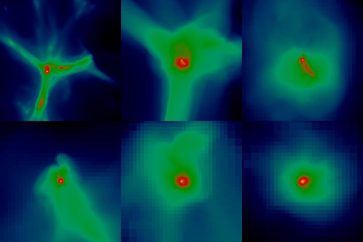
Figure 1: Zoom on projected mass-weighted baryon density by factors of four for a representative Population III protostar formation calculation at the last simulation output. At this redshift ($z=19.28$), the maximum density was $\sim 10^{12}$ cm^-3 with a cosmic mean density of $\simeq 0.003$ cm^-3, for an overall density increase of 15 orders of magnitude. Top left: view is 1320 pc across. Top center: 330 pc. Top right: 82.5 pc. Bottom left: 20.6 pc. Bottom center: 5.2 pc. Bottom right: 1.29 pc. Note that all sizes are in proper parsecs at $z=19.28$. In all panels yellow represents high densities and blue represents low density, with the color table relative in each frame.

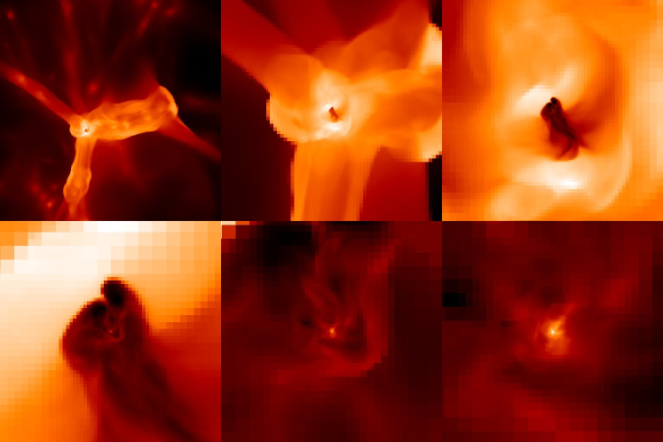
Figure 2: Zoom on projected mass-weighted baryon temperature by factors of four in a representative Population III protostar formation calculation at the last simulation output. The collapse redshift is $z=19.28$ and the simulation and spatial sizes of each panel are the same as in Figure 1. In all panels white represents high temperatures and dark colors represent low temperatures. The color table is relative in each frame.

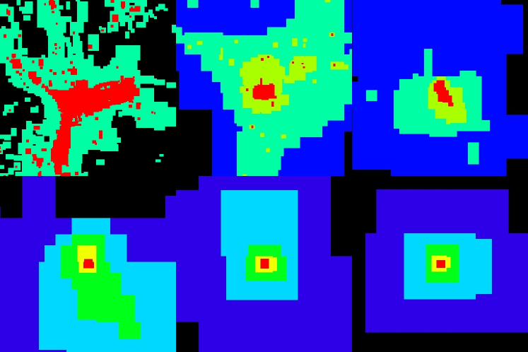
Figure 3: Zoom on projected maximum level in a representative Population III protostar formation calculation at the last simulation output. The spatial scale for each panel and simulation are the same as in Figure 1. The maximum projected level in each panel is as follows. Top left: Level 6. Top center: Level 8. Top right: Level 10. Bottom left: Level 12. Bottom center: Level 14. Bottom right: Level 16. In each panel the highest level grid is represented is in red, second highest in yellow, and so on. The highest level of resolution at this time is $L=22$.

Figures 4 through 6 show the evolution of radial profiles of several spherically averaged, mass-weighted baryon quantities of a representative primordial protostar from approximately the onset of halo collapse until the formation of a fully molecular core. The halo begins its collapse at $z=18.05$ (approximately $2.04\times 10^{8}$ years after the Big Bang) and ends its collapse $6.294\times 10^{6}$ years later, at $z=17.67$. Figure 4 shows the spherically-averaged baryon number density, temperature, and enclosed mass as a function of radius, and the specific angular momentum of the baryon gas as a function of enclosed mass. Figure 5 shows the molecular hydrogen fraction, electron fraction, $H^{-}$ fraction and circular velocity as a function of radius. Figure 6 shows the ratios of gas cooling time to sound crossing time, cooling time to system dynamical time, sound crossing time to dynamical time, and radial velocity as a function of radius. The lines in all of these plots are chosen such that the same line thickness and type corresponds to the same time in each panel.

We begin to follow the evolution of the halo at $z=18.05$, when the central hydrogen number density has reached $n_{H}\sim 10^{3}$ particles per cubic centimeter (black solid line in all plots). This corresponds to a core with a radius of $\sim 1$ parsec and a mass of a few thousand solar masses, which is accreting gas at a significant rate. The molecular hydrogen fraction within this core is slightly less than $10^{-3}$ but is still enough to rapidly cool the center of the halo to $\sim 200$ Kelvin at a cooling rate proportional to the square of the gas density. The gas cannot cool below this temperature because of the sharp decrease in the cooling rate of molecular hydrogen below $\simeq 200$ Kelvin. This core is the high-redshift equivalent of a molecular cloud core. The halo “loiters” for approximately six million years as the amount of molecular hydrogen is slowly built up to a mass fraction of a few times $10^{-3}$ and the central density increases. As can be seen from Figure 6, the cooling time in the halo core is significantly larger than both the dynamical time and sound crossing time at this epoch, so the core can be quite reasonably said to be quasistatically evolving. It is useful to compare the late-time evolution of a Population III minihalo to the Shu (1977) isothermal sphere model of cloud collapse, which is most commonly applied to quasistatic cores in galactic molecular clouds.

As the gas density passes roughly $n_{H}\sim 10^{4}$ cm^-3 the ro-vibrational levels of H₂ are populated at their thermodynamic equilibrium values and the cooling rate becomes independent of density, which corresponds to an increase in gas temperature with increasing density (as can be seen by the blue and green solid lines in the temperature vs. radius plot in Figure 4). As the temperature increases the cooling rate again begins to rise, leading to an increase in the inflow velocities of gas. This is easily explained by the Shu model, as the infall of gas onto the quasistatic halo is moderated by the sound speed, and the accretion rate $\dot{m}$ scales as the sound speed cubed. Examination of the plot of enclosed mass vs. radius in Figure 4 shows that at this point the enclosed gas mass has exceeded the Bonnor-Ebert critical mass, which is defined as $M_{BE}=1.18M_{\odot}(c_{s}^{4}/G^{3/2})P_{ext}^{-1/2}$, where $c_{s}$ is the local sound speed and $G$ is Newton’s constant. This is the critical mass at which an isothermal sphere of gas with an external pressure $P_{ext}$ becomes gravitationally unstable and undergoes collapse. This occurs in this halo at a mass scale of $\sim 1000$ M_⊙.

When the central density of the cloud core becomes sufficiently large ($n_{H}\sim 10^{8}$ cm^-3) the three-body H₂ formation process takes over, resulting in a rapid increase in the molecular hydrogen fraction from a few times $10^{-3}$ to essentially unity. The halo densities also cause a rapid drop in the $H^{-}$ and electron fractions, though the dominance of the 3-body channel makes the $H^{-}$ channel for molecular hydrogen formation unimportant. This causes a huge increase in the cooling rate, which results in a rapid drop in temperature of the center of the halo, allowing it to contract and causing an increase in central density of $n_{H}\sim 10^{15}$ cm^-3 in only $\sim 2\times 10^{4}$ years. The infall velocity of gas to the center of the halo peaks at the same radius as the temperature, and drops within that radius (r $\simeq 10^{-3}$ pc). At a mass scale of $\sim 1$ M_⊙ a protostellar cloud core forms which is completely molecular and has gas accreting onto it supersonically. At this point the optical depth of the halo core becomes close to unity to molecular hydrogen ro-vibrational line emission, so we terminate the simulation because the assumption of optically thin radiative cooling used in our code is no longer correct. Note also the change from supersonic back to subsonic accretion at very small radii in Figure 6 (d) is not an accretion shock onto a protostar – rather, it is a numerical effect due to the flow converging to a single point in a grid cell with finite resolution.

Panel (d) in Figures 4 through 6 shows the dynamical evolution of the collapsing halo. These plots show the spherically-averaged, mass-weighted, specific angular momentum as a function of enclosed baryon mass and the spherically-averaged, mass-weighted, baryon radial velocity and circular velocity as a function of radius. Though the angular momentum of the gas within the halo core (m${}_{b}\lesssim 10^{3}$ M_⊙) is conserved overall, there is clear evidence for transport of angular momentum outward. This effect can be shown to be physical (as opposed to a numerical effect), and is due to a combination of turbulent transport of high angular momentum gas outward and a “segregation effect,” where low angular momentum gas tends to move inward during halo collapse. A detailed discussion of this issue is deferred to the second paper in this series (O’Shea, Norman & Li 2006, in preparation).

The thin dot-dashed lines in the plots of spherically-averaged baryon infall velocity and cylindrically-averaged (in shells along the axis of rotation) baryon circular velocity (the bottom right panel in Figure 5 correspond to the locally-determined sound speed and Keplerian orbital velocities at the final timestep, respectively. The infall of gas is locally subsonic until very late times, when the core has reached densities of $n_{H}\sim 10^{12}$ cm^-3 and an H₂ fraction approaching unity. The infall velocities then become locally supersonic, but decrease rapidly within this radius because a protostellar cloud core has formed which the gas is accreting onto, and has formed a standing shock. At no point in the simulated evolution is the gas within the halo core rotationally-supported: the initial distribution of gas velocities is such that gas in the core has very little angular momentum, and what little exists is efficiently transported outward.

It is useful to examine the relevant chemical, thermal and dynamical timescales of the collapsing halo. The ratios of cooling time to sound crossing time (calculated as a mass-weighted mean in spherically averaged radial shells) as a function of radius, cooling time to dynamical time (calculated assuming spherical symmetry), and sound crossing time to dynamical time are plotted in Figure 6. Within the core of the halo ($r\sim 1$ parsec) the sound crossing time ($t_{cross}$) is slightly less than the dynamical time ($t_{dyn}$) for the majority of the evolution time of the halo, while the cooling time ($t_{cool}$) is somewhat longer than both of these timescales, but generally only by a factor of a few. If $t_{cross}\ll t_{dyn}$ the halo is stable against collapse because the halo can easily equilibrate its pressure to compensate for collapsing gas. If $t_{cross}\gg t_{dyn}$, the system cannot come into equilibrium and is in free-fall. In this case, $t_{cross}\approx t_{dyn}<t_{cool}$, and the system is undergoing a quasistatic collapse. This can also be seen by examining the evolution of the radial infall velocity as a function of radius in Figure 6, where the radial infall velocity is subsonic until the very last portion of the core’s evolution, when it becomes locally supersonic. This is triggered by a dramatic increase in the molecular hydrogen fraction, and a corresponding rapid decrease in the cooling time. In the center of the halo at the last few data outputs, the cooling time becomes shorter than both the dynamical time and sound crossing time, creating a situation where gas is essentially free-falling onto the central protostar.

As in ABN02, we carefully examine the collapsing protostellar cloud core for signs of fragmentation. This might be expected due to chemothermal instabilities caused by the rapid formation of molecular hydrogen via the 3-body process and the resulting rapid increase in cooling rate (Silk 1983). However, the sound crossing time within the core is less than the H₂ formation timescale until the last output time, allowing mixing to take place and preventing the formation of large density contrasts. By the time that the H₂ formation timescale becomes shorter than the sound crossing time, the core is fully molecular and therefore stable against this chemothermal instability. For an alternate explanation, see Omukai & Yoshii (2003).

Figure 4: Evolution of spherically-averaged values for baryon number density (a), baryon temperature (b), and enclosed baryon mass (c) as a function of radius and spherically-averaged baryon specific angular momentum as a function of enclosed mass (d) of a representative primordial protostar. The thick solid black line in each panel corresponds to spherically averaged radial profile of each quantity the onset of halo collapse, at $z=18.05$ (approximately $2\times 10^{8}$ years after the Big Bang). Thick dotted line: the state of the halo $5.97\times 10^{6}$ years after that. Thick short-dashed line: $1.89\times 10^{5}$ years later. Thick long-dashed line: $1.21\times 10^{5}$ years later. Thick dot-dashed line: $6,810$ years later. Thin solid line: $782$ years later. Thin dotted line: $151$ years later. Thin short-dashed line: $58$ years later. Thin long-dashed line: $14$ years later, at a final output redshift of $z=17.673$. The total time spanned by the lines in these panels is $6.294\times 10^{6}$ years. The black dot-dashed line in the bottom left panel is the Bonnor-Ebert critical mass calculated at the last timestep.

Figure 5: Evolution of spherically averaged radial profiles of molecular hydrogen fraction (a), electron fraction (b), $H^{-}$ fraction (c) and baryon circular velocity (d) as a function of radius of a representative primordial protostar. The lines correspond to the same times as in Figure 4 and are of the same simulation. The black dot-dashed line in the plot of baryon circular velocity vs. time is the Newtonian circular velocity computed from the radius and enclosed baryon mass at the last timestep.

Figure 6: Evolution of the ratio of gas cooling time to sound crossing time (a), gas cooling time to system dynamical time (b), sound crossing time to system dynamical time (c) and baryon radial velocity (d) as a function of radius of a representative primordial protostar. These quantities are mass-weighted and spherically-averaged, and the lines correspond to the same times as in Figure 4 and are of the same simulation. The black dot-dashed line in the plot of radial velocity as a function of radius is the sound speed calculated using the local baryon temperature in each radial bin at the last simulation timestep.

As discussed previously, at the time when the simulation is stopped due to a breakdown in the assumption of optically thin radiative cooling at the center of the protostellar cloud , a fully-molecular core with a mass of $\sim 1$ M_⊙ has formed and is accreting gas supersonically. The spherically-averaged accretion time at the last output timestep, plotted as a function of enclosed gas mass, is shown as the thick solid line in Figure 7. The accretion time is defined as $t_{acc}\equiv M_{enc}/\dot{m}$, where $M_{enc}$ is the enclosed baryon mass and $\dot{m}\equiv 4\pi r^{2}\rho(r)v(r)$, with $\rho(r)$ and $v(r)$ being the spherically-averaged, mass-weighted baryon density and velocity as a function of radius, and $v(r)$ defined as being positive towards the center of the halo. The thick dashed line is the accretion time as determined by taking the local accretion rate from the Shu isothermal collapse model, $\dot{m}_{Shu}=m_{0}c_{s}^{3}/G$, where $m_{0}$ is a dimensionless constant of order unity (we use $m_{0}=0.975$, as derived by Shu), $c_{s}$ is the sound speed, and $G$ is the gravitational constant. This value of $\dot{m}$ is calculated in each bin and the accretion time is plotted as $M_{enc}/\dot{m}_{Shu}$. The dot-long dashed line is the Kelvin-Helmholtz time for a Population III star with a mass identical to the enclosed mass calculated assuming a star with a main sequence radius and luminosity as given by Schaerer (2002). The short dash-long dashed line is the lifetime of a massive primordial star as calculated by Schaerer, assuming no mass loss. Note that this fit only covers the mass range $5-500$ M_⊙, but the lifetime of massive stars with a mass greater than $500$ M_⊙ is roughly constant. The dot-short dashed line is the baryon accretion time for the result in ABN02.

We can see that the accretion rates in our model and in ABN02 are well-approximated by the Shu model for $M_{enc}\lesssim 10^{3}$ M_⊙, which is the Bonner-Ebert mass scale of the collapsing core. All three curves predict that $100-200$ M_⊙ of gas will accrete within the Kelvin-Helmholtz time of the Population III star, implying that it will be at least this massive. As we will see in the next section, the similarity of these curves is somewhat fortuitous, as we find substantial variation of accretion times within our suite of models.

Figure 7: Baryon gas accretion time as a function of enclosed baryon mass for simulation L0_30A. This is defined as $M_{enc}/\dot{m}$, where $M_{enc}$ is the enclosed baryon mass and $\dot{m}\equiv 4\pi r^{2}\rho(r)v(r)$, with $\rho(r)$ and $v(r)$ being the baryon density and velocity as a function of radius, and $v(r)$ defined as being positive towards the center of the halo. The thick solid line is the baryon accretion time for this simulation. The thick dashed line is the accretion time as determined by taking the accretion rate from the Shu isothermal collapse model, $\dot{m}_{Shu}=m_{0}c_{s}^{3}/G$, where $m_{0}$ is a dimensionless constant of order unity, $c_{s}$ is the sound speed, and $G$ is the gravitational constant. This value of $\dot{m}$ is calculated in each bin and the accretion time is plotted as $M_{enc}/\dot{m}_{Shu}$. The thin line with the label “KH” is the Kelvin-Helmholtz time for a Population III star with a mass identical to the enclosed mass, as calculated from the results given by Schaerer. The thin line labeled “$t_{*}$” is the lifetime of a massive primordial star assuming no significant mass loss, as calculated by Schaerer. Note that this fit only covers the mass range $5-500$ M_⊙, but $t_{*}\simeq$ constant for $M_{*}>500$ M_⊙. The thin dot-short dashed line labeled “ABN02” is the baryon accretion time for the result in ABN02. The plot here corresponds to the last output dataset, corresponding to the thin, long-dashed line in Figures 4 through 6.

4 Comparison of multiple realizations

Another important issue relating to studies of the formation of Population III stars in a cosmological context is the consistency of the results over a range of simulation parameters. As discussed in the introduction to this article, previously published high dynamical range calculations of Pop III star formation have concentrated upon a single cosmological realization. While this is an important first step, it neglects possible systematic effects and also allows for error due to small number statistics.

In this section we attempt to address some of these issues. Twelve simulations are set up as described in Section 2.2. Each simulation has the same cosmological parameters but a different cosmological realization (i.e. large scale structure). Four simulations in each of three box sizes ($0.3,0.45$, and $0.6$ h^-1 comoving Mpc) are performed, with the results shown in Figures 8 through 19.

4.1 Halo bulk properties

Figures 8 - 10 display several mean properties of the halos. In each panel information for each simulation is plotted as an open shape which assigned according to box size as described in the figure captions. The filled-in shapes correspond to mean values for all simulations of a given box size (with shapes again corresponding to the box size), and the open circle corresponds to the mean of all twelve of the simulations together. All quantities discussed in this section can be found in Tables 2 and 3.

Panel (a) of Figure 8 shows the virial mass of each halo calculated using the virial density fitting function of Bryan & Norman (1998) at the time of protostellar cloud collapse plotted against the redshift of collapse. Though there is a large amount of scatter in virial mass overall, with the smallest halo having a mass of $1.36\times 10^{5}$ M_⊙ and the largest $6.92\times 10^{5}$ M_⊙, the average virial mass in each box size is virtually identical. The mean virial mass of all twelve of the halos is $3.63\times 10^{5}$ M_⊙, which is significantly lower than the halo mass of $7\times 10^{5}$ M_⊙ in ABN02 and the minimum mass of $5\times 10^{5}$ h^-1 M_⊙ found by Yoshida et al. (2003) (note that the value found by ABN02 is from a different cosmology with much higher values of $\Omega_{m}$ and $\Omega_{b}$, yet is still within the scatter of halo virial masses found in this work). In contrast to the virial mass, there is an apparent trend in earlier collapse time (large collapse redshift) as a function of box size, with the 0.45 and 0.6 h^-1 Mpc boxes collapsing at a mean redshift of $z\simeq 27.5$ and the 0.3 h^-1 Mpc boxes collapsing at a mean redshift of $z\simeq 22$. This can be understood as a result of the larger boxes sampling a much larger volume of the universe. The first halo to collapse in the larger volume tends to be a statistically rarer density fluctuation that collapses at a higher redshift. A consequence of this can be seen in panel (b) of Figure 8, which shows the mean baryon temperature in each halo as a function of collapse redshift. As with the plot of virial mass vs. collapse redshift, there is a significant amount of scatter in the results, but a clear trend of increased overall halo temperature with collapse redshift is apparent. This is explainable in terms of virial properties of the halo. The virial temperature scales as $T_{vir}\sim M_{vir}^{2/3}(1+z)$, so halos with a constant virial mass will be hotter at higher redshifts, as observed in this plot.

Figure 8: Plots of basic halo quantities for 12 different cosmological random realizations. Panel (a): halo virial mass vs. protostar collapse redshift. Panel (b): mean mass-weighted halo baryon temperature vs. collapse redshift. Panel (c): ($(<T>_{m}/(1+z))^{3/2}$ vs. halo virial mass. Panel (d): halo mean baryon temperature vs. halo virial temperature. In each plot, open triangles, squares and hexagons correspond to simulations with 0.3 h^-1 Mpc, 0.45 h^-1 Mpc and 0.6 h^-1 Mpc comoving box size, respectively. The filled shapes corresponds to the average value for simulations with that box size. The open circle corresponds to the average for all simulations together. The upper and lower dashed lines in panels (c) and (d) correspond to the scaling relation one would expect if $<T>_{m}$ = $T_{vir}$ and $<T>_{m}$ = 0.5 $T_{vir}$, respectively.

The virial scaling of the mean halo baryon temperature vs. halo virial mass ($(<T>_{m}/(1+z))^{3/2}$ vs. $M_{vir}$) is plotted in panel (c) of Figure 8, and the mean halo temperature versus the halo virial temperature is plotted in panel (d). The upper and lower dashed lines in both panels correspond to the scaling relation one would expect if $<T>_{m}$ = $T_{vir}$ and $<T>_{m}$ = 0.5 $T_{vir}$, respectively. Since the actual observed mean halo temperatures are significantly lower than the virial temperature, as shown in panel (d), one can infer that radiative cooling plays a significant role in the condensation of gas in these halos despite the generally poor cooling properties of primordial gas at low temperature. If radiative cooling were completely unimportant the mean halo baryon temperature would be approximately the virial temperature for all halos. Examination of panels (c) and (d) together show that the temperature evolution of the halos is consistent with virial scaling, given the importance of radiative cooling.

Figure 9 shows the relationship of the angular momentum in the halos with various quantities. The angular momentum of a cosmological halo can be described as a function of the dimensionless spin parameter, $\lambda\equiv J|E|^{1/2}/GM^{5/2}$, where J is angular momentum, E is the total energy, G is the gravitational constant and M is the halo mass. This is roughly equivalent to the ratio of the angular momentum of the halo to the angular momentum needed for the halo to be rotationally supported.

Figure 9: Plots of basic halo quantities for 12 different cosmological random realizations. Panel (a): gas spin parameter vs. dark matter spin parameter. Panel (b): dark matter spin parameter vs. halo collapse redshift. Panel (c): gas spin parameter vs. halo virial mass. Panel (d): dark matter spin parameter vs. halo virial mass. In each plot, open triangles, squares and hexagons correspond to simulations with 0.3 h^-1 Mpc, 0.45 h^-1 Mpc and 0.6 h^-1 Mpc comoving box sizes, respectively. The filled shapes corresponds to the average value for simulations with that box size. The open circle corresponds to the average for all simulations together.

Panel (a) of Figure 9 shows the gas and dark matter spin parameters plotted against each other for the halo in each simulation that forms the primordial protostellar core, at the epoch of collapse. The mean value of the dark matter spin parameter is approximately 0.05. The gas spin parameter tends to have somewhat lower values, with a mean of $\simeq 0.035$, but, considering the number of halos examined, is consistent with the dark matter spin parameter. There appears to be some overall positive correlation between the dark matter and baryon spin parameters (e.g. halos with higher overall dark matter angular momentum tend to have higher overall baryon angular momentum) but there is considerable scatter. In all cases the spin parameters are much less than one, which suggests that the halos have little overall angular momentum. The measured range and distribution of the spin parameters agree well with previous analytical and numerical results which predict typical values for the spin parameter of $0.02-0.1$, with a mean value of $\simeq 0.05$  (Barnes & Efstathiou 1987; Gardner 2001; van den Bosch et al. 2002; Yoshida et al. 2003).

Panel (b) of Figure 9 plots dark matter spin parameter vs. collapse redshift of the halo. There is no evidence that the collapse redshift systematically depends on the spin parameter. Panels (c) and (d) of Figure 9 plot the baryon and dark matter spin parameters against the halo virial mass. As with the other quantities examined, there is considerable scatter in the distributions, but no evidence for a clear relationship between halo virial mass and either gas or dark matter spin parameter. In all of the panels of this figure there is no evidence for any systematic effect due to box size or collapse redshift.

Figure 10 plots the angle between the overall dark matter and baryon angular momentum vectors ($\theta$) versus several different quantities. Panel (a) plots $\theta$ vs. halo virial mass at the time of formation of the Pop III protostar in each halo. Overall, the average value for $\theta$ is approximately 25 degrees, which is consistent with recent numerical simulations (van den Bosch et al. 2002; Yoshida et al. 2003). There is a great deal of scatter in $\theta$, which is also consistent. There is no evidence for correlation between $\theta$ and halo virial mass. Panel (b) plots $\theta$ vs. collapse redshift for each simulation, and panels (c) and (d) plot the gas and dark matter spin parameters vs. $\theta$, respectively. There appears to be no correlation between $\theta$ and collapse redshift or the gas or dark matter spin parameters, and no evidence of there being any systematic effect due to box size.

Figure 10: Plots of basic halo quantities for 12 different cosmological random realizations. Panel (a): Theta (angle between gas and dark matter angular momentum vectors) vs. halo virial mass. Panel (b): theta vs. halo collapse redshift. Panel (c): gas spin parameter vs. theta. Panel (d): dark matter spin parameter vs. theta. In each plot, open triangles, squares and hexagons correspond to simulations with 0.3 h^-1 Mpc, 0.45 h^-1 Mpc and 0.6 h^-1 Mpc comoving box sizes, respectively. The filled shapes corresponds to the average value for simulations with that box size. The open circle corresponds to the average for all simulations together.

4.2 Halo radial profiles

In addition to plots of mean halo properties, it is very useful to look at more detailed information about each halo. Figures 11 through 15 show spherically-averaged, mass-weighted radial profiles of several baryon quantities in eleven of the twelve simulations (one simulation crashed and could not be restarted before reaching a high enough density). Since the cores of the most massive halo in each simulation collapse at a range of redshifts, we choose to compare them at a fixed point in the halo’s evolution, as measured by the peak central baryon density in the protostellar cloud, which is roughly analogous to a constant point in the evolution of the protostar. In each of the figures discussed below, panel (a) shows radial profiles for all of the simulations plotted together. Panel (b) shows only the results for the 0.3 h^-1 Mpc box, panel (c) shows only results for the 0.45 h^-1 Mpc box, and panel (d) shows only results for the 0.6 h^-1 Mpc box. Line of a given line type and weight correspond to the same simulation in all figures.

Figure  11 shows the plots of number density as a function of radius for eleven simulations, shown at approximately the same point in their evolution. There is remarkably little scatter in the density profiles for all of the simulations (less than 1 dex at any given radius), and the density profiles all tend towards $\rho(r)\sim r^{-2.2}$. It was shown by Bodenheimer & Sweigart (1968) that for a cloud of gas that is nearly isothermal and slowly rotating and which has negligible support from a magnetic field, the subsonic evolution of the gas will tend to produce a $1/r^{2}$ density distribution as long as the thermal pressure remains approximately in balance with the gravitational field. In particular, Chandrasekhar (1939) showed that a molecular cloud core which forms at subsonic speeds will tend towards the density distribution of a singular isothermal sphere,

$$\rho(r)=\frac{c_{s}^{2}}{2\pi Gr^{2}}$$ (1)

where $c_{s}\equiv(kT/m)^{1/2}$ is the isothermal sound speed, T, k, and m are the temperature, Boltzmann’s constant, and mean molecular weight of the gas, respectively, and and r is the radius. Since the halos generally have low angular momentum (as seen in Figure 9) and magnetic fields are completely neglected in these simulations, it is reasonable that the density should go as $\rho(r)\sim r^{-2}$ in all of the simulations, with the deviation from $r^{-2}$ being a result of the effective equation of state of the primordial gas (Omukai & Nishi (1998)). The overall normalization of the density profiles also agrees very well. This can be understood as a result of the cooling properties of hydrogen gas. Each of the halos examined in this figure has the same composition, and therefore is cooled by the same mechanism. Only a small amount of molecular hydrogen is needed to cool the gas relatively efficiently, suggesting that in a halo that is in a somewhat stable equilibrium the gas temperature at low densities should be approximately constant for different halos, independent of the molecular hydrogen fraction. At densities above $n_{H}\simeq 10^{4}$ cm^-3 the cooling rate becomes independent of density and the halo enters a “loitering” phase, where a slow buildup of mass occurs. Once a Bonnor-Ebert mass of gas accumulates, the halo core becomes gravitationally unstable and begins to evolve very rapidly, so small differences in the initial molecular hydrogen fraction become magnified (as discussed later in this section). The scatter in densities at a given radius is related to the scatter in virial masses, and there is no systematic effect with collapse redshift.

Figure 11: Panel (a): mass weighted, spherically-averaged baryon number density as a function of radius for 11 different cosmological random realizations, chosen at an output time where peak baryon density values are approximately the same. (b-d): Density profiles separated according to box size. (b): 0.3 h^-1 Mpc, (c) 0.45 h^-1 Mpc, (d) 0.6 h^-1 Mpc (comoving). One of the 0.45 h^-1 Mpc simulations has been omitted since the simulation crashed before reaching a comparable density value. Line thicknesses and types correspond to individual simulations. L0_3A: Thick solid line. L0_3B: Thick dotted line. L0_3C: Thick short-dashed line. L0_3D: Thick long-dashed line. L0_45A: Thick dot-short dashed line. L0_45B: Thick dot-long dashed line. L0_45C: Thin solid line. L0_45D: Thin dotted line. L0_6A: Thin short-dashed line. L0_6B: Thin long-dashed line. L0_6C: Thin dot-short dashed line. L0_6D: Thin dot-long dashed line.

Figure 12 shows the baryon temperature as a function of radius. At radii outside of $\sim 1$ parsec, the temperature profiles are similar between all of the simulations, though halos forming at higher redshifts tend to have a higher overall temperature. At smaller radii there is significant scatter in core temperature of the simulations (for a fixed density), with a systematic trend towards halos forming in larger boxes having a lower overall core temperature. Examination of Figure 13 plots molecular hydrogen mass fraction as a function of radius, and shows that halos which form at higher redshift have systematically larger H₂ mass fractions, though this effect is much more pronounced in the core of the halo than in the envelope. This difference in molecular hydrogen fraction can be understood as a result of the overall halo temperature. The rate at which molecular hydrogen is produced at low densities is limited by the availability of free electrons, as described by Tegmark et al. (1997). The mean fraction of free electrons available in the primordial gas is a function of baryon temperature, with larger temperatures corresponding to larger electron fractions. On the other hand, the rate at which molecular hydrogen forms via the $H^{-}$ channel declines at high temperatures. Since the limiting reaction in the formation of molecular hydrogen via the $H^{-}$ channel is the formation of free electrons, this reaction dominates, and it can be shown using a simple one-zone calculation following the nonequilibrium primordial chemistry that molecular hydrogen production is maximized at $\sim 1000~{}$K. Halos with higher overall baryon temperatures will have systematically higher molecular hydrogen fractions. Once the core of the halo begins to collapse to very high densities small differences in the molecular hydrogen fraction are amplified, resulting in a general trend towards halos with higher overall baryon temperatures having higher H₂ fractions in their cores, and thus lower central temperatures.

Figure 12: Mass weighted, spherically-averaged baryon temperature as a function of radius for 12 different cosmological random realizations, chosen at an output time where peak baryon density values are approximately the same. (a) All 12 simulations, (b) $L_{box}=$ 0.3 h^-1 Mpc, (c) $L_{box}=$ 0.45 h^-1 Mpc, and (d) $L_{box}=$ 0.6 h^-1 Mpc (comoving). Line thicknesses and types are identical to those shown in Figure 11.

Figure 13: Mass weighted, spherically-averaged baryon molecular hydrogen fraction as a function of radius for 12 different cosmological random realizations, chosen at an output time where peak baryon density values are approximately the same. (a) All 12 simulations, (b) $L_{box}=$ 0.3 h^-1 Mpc, (c) $L_{box}=$ 0.45 h^-1 Mpc, and (d) $L_{box}=$ 0.6 h^-1 Mpc (comoving). Line thicknesses and types are identical to those shown in Figure 11.

Figure 14 plots the mean baryon radial velocity as a function of radius. This figure shows that there is a clear systematic effect present, where halos forming in simulations with larger boxes having a significantly lower overall radial velocity at small radii. This translates directly to a lower overall accretion rate onto protostellar forming in halos in larger simulation volumes, which is discussed more thoroughly in Section 4.3. As discussed in Section 3, this can be understood using the Shu isothermal sphere model, where subsonic collapse of gas onto the core of the sphere occurs at a rate controlled by the sound speed. Since the core temperatures are lower overall in the large simulation volumes, this translates to a lower sound speed and overall lower radial infall velocity. A lower infall velocity implies a lower accretion rate, which may have profound implications for the Population III IMF – and are discussed elsewhere in this work.

Figure 14: Mass-weighted, spherically-averaged baryon radial velocity as a function of radius for 12 different cosmological random realizations, chosen at an output time where peak baryon density values are approximately the same. (a) All 12 simulations, (b) $L_{box}=$ 0.3 h^-1 Mpc, (c) $L_{box}=$ 0.45 h^-1 Mpc, and (d) $L_{box}=$ 0.6 h^-1 Mpc (comoving). Line thicknesses and types are the same as in Figure 11.

Figure 15 shows the baron circular velocity in each halo as a function of radius. There is a great deal of scatter in this relationship, though there is no clear trend with simulation box size. In all cases the overall circular velocity is significantly less than the Keplerian orbital velocity, which agrees with our previous observation that the halos have generally low angular momentum.

Figure 15: Mass weighted, cylindrically-averaged baryon circular velocity as a function of radius for 12 different cosmological random realizations, chosen at an output time where peak baryon density values are approximately the same. (a) All 12 simulations, (b) $L_{box}=$ 0.3 h^-1 Mpc, (c) $L_{box}=$ 0.45 h^-1 Mpc, and (d) $L_{box}=$ 0.6 h^-1 Mpc (comoving). Line thicknesses and types are the same as in Figure 11.

4.3 Protostellar accretion rates

Figures 16 –  20 show baryon properties relating to the accretion rate onto the forming protostellar core. Many of these properties are also detailed in Tables 2 and 3. Figure 16 shows the mass-weighted, spherically averaged accretion time as a function of enclosed gas mass for 11 of the 12 cosmological simulations. There is a 2 order of magnitude scatter in accretion rates, with a trend towards lower accretion rates (longer accretion times) in simulations that have larger box sizes. Figure 17 shows the mass-weighted, spherically averaged accretion rate onto the protostellar core as a function of time for all twelve cosmological simulations. The time on the x-axis is calculated by summing up $\Delta M_{b}/\dot{m}$ on spherical shells, where $\Delta M_{b}$ is the amount of baryon gas and $\dot{m}$ is the instantaneous gas accretion rate at that shell, starting at the center of the halo and assumes no feedback. Although this is only a crude estimate of the true accretion rate, we see that all curves rise quickly to a maximum accretion rate at $t\sim 10^{4}$ year, and decline thereafter, in agreement with the results of  Bromm & Loeb (2004) and Yoshida et al. (2006).

Figure 16: Mass-weighted, spherically averaged gas accretion time as a function of enclosed baryon mass for 12 different cosmological random realizations, chosen at an output time where peak baryon density values are approximately the same. Panel (a): All simulations plotted together. Panel (b): 0.3 h^-1 Mpc box simulations. Panel (c): 0.45 h^-1 Mpc box simulations. Panel (d): 0.6 h^-1 Mpc box simulations. Individual simulations are identified by line thicknesses and types identical to those in Figure 11. The baryon accretion time is defined as $T_{acc}\equiv M_{enc}/\dot{m}$, where $M_{enc}$ is the enclosed baryon mass and $\dot{m}\equiv 4\pi r^{2}\rho(r)v(r)$, with $\rho(r)$ and $v(r)$ being the spherically-averaged baryon density and velocity as calculated on spherical shells, and $v(r)$ defined as being positive towards the center of the halo. The dot-long dashed line in each panel is the Kelvin-Helmholtz time for a Population III star with a mass identical to the enclosed mass, as calculated from the results given by Schaerer. The long dash-short dashed line is the lifetime of a massive primordial star assuming no significant mass loss, as calculated by Schaerer. Note that this fit only covers the mass range $5-500$ M_⊙, by $t_{*}\simeq$ constant for $M_{*}>500$ M_⊙. The dot-short dashed line in each panel is the baryon accretion time for the result in ABN02. The upper and lower diagonal thin solid lines are the accretion times for constant accretion rates of $10^{-3}$ and $10^{-2}$ M_⊙/yr, respectively.

Figure 17: Mass-weighted, spherically averaged gas accretion rate as a function of time for all 12 cosmological random realizations. Panel (a): All simulations plotted together. Panel (b): 0.3 h^-1 Mpc box simulations. Panel (c): 0.45 h^-1 Mpc box simulations. Panel (d): 0.6 h^-1 Mpc box simulations. Line thicknesses and types are the same as in Figure 11. The accretion rate is defined as $\dot{m}\equiv 4\pi r^{2}\rho(r)v(r)$, with $\rho(r)$ and $v(r)$ being the spherically-averaged baryon density and velocity as calculated on spherical shells, and $v(r)$ defined as being positive towards the center of the halo. The time is calculated by summing $\Delta M_{b}/\dot{m}$ in each shell starting at the center of the halo and working outward, and plotting vs. $\dot{m}$.

Figure 18 shows the mass accretion rate vs. halo virial mass, molecular hydrogen fraction vs. halo virial mass, mass accretion rate vs. molecular hydrogen fraction, and mass accretion rate vs. halo collapse redshift. In all panels in this figure the molecular hydrogen fraction is taken as an average over all gas within the virial radius, and accretion rate values are taken instantaneously at spherically-averaged radial shells corresponding to an enclosed baryon mass of 100 M_⊙ (Note that the trends here do not change significantly if this mass shell is varied by a factor of 10 in either direction, so the results are quite robust). This figure shows that there is a general trend of higher mass accretion rates with increasing halo mass. though there is a great deal of scatter, and the variance is virial mass is not that large. There is no evidence for a comparable trend in the molecular hydrogen fraction with virial mass. The bottom panels show that there is a strong relationship between the mass accretion rate and the mean molecular hydrogen fraction of the halo and the redshift of collapse. The accretion rate steadily decreases with increasing H₂ fraction, and increases with decreasing redshift (increasing time).

Figure 18: Panel (a): Mass accretion rate ($\dot{m}$) vs. halo virial mass. Panel (b): Molecular hydrogen fraction vs. halo virial mass. Panel (c): Mass accretion rate vs. molecular hydrogen fraction. Panel (d): Mass accretion rate ($\dot{m}$) vs. halo collapse redshift. The $H_{2}$ fraction is taken as an average over all gas within the virial radius. All values of accretion rate are taken instantaneously at spherically-averaged radial shells corresponding to an enclosed gas mass of 100 $M_{\odot}$. In each plot, open triangles, squares and hexagons correspond to simulations with 0.3 h^-1 Mpc, 0.45 h^-1 Mpc and 0.6 h^-1 Mpc comoving box sizes, respectively.

The plots shown in Figure 19 help to explain these trends. This figure shows the mean halo temperature scaled by virial mass, core molecular hydrogen fraction, and core baryon temperature as a function of collapse redshift, and the core temperature as a function of molecular hydrogen fraction. All “core” quantities are measured at the epoch of collapse at a proper radius of 0.1 pc, though changing this value does not change the results significantly. There is a clear relationship between collapse redshift and mean temperature, with temperature decreasing with decreasing collapse redshift (increasing time). This is explainable, as discussed previously, as a simple virial scaling: halo masses at the time of protostellar core formation stay approximately constant with redshift, and since the virial temperature scales as $T_{vir}\sim M_{vir}^{2/3}(1+z)$, higher redshift halos have systematically higher temperatures. The limiting reaction in the formation of molecular hydrogen at low ($\lesssim 10^{8}$ cm^-3) densities is the formation of H^-, which scales as $\sim T^{0.88}$. This suggests that halos whose gas is overall warmer (up to $\sim 1000$ K, where high temperatures begin to collisionally dissociate H₂) more molecular hydrogen will be produced. This is borne out in the plot of core molecular hydrogen fraction vs. collapse redshift, where halos that form at later times (and in overall cooler objects) have less molecular hydrogen. The results of this are shown quite plainly in the plot of core temperature vs. collapse redshift, where objects that form later have higher core temperatures and hence higher accretion rates, since $\dot{m}\sim T^{3/2}$. This relationship is shown in a different way by the plot of core temperature vs. core H₂ fraction in Figure 19, where there is a clear correlation between decreasing temperature with increasing H₂ fraction.

Figure 19: Panel (a): $<T>_{m}/M_{vir}^{2/3}$ vs. $1+z_{coll}$ ($z_{coll}$ is the halo collapse redshift). Panel (b): Core $H_{2}$ fraction vs. collapse redshift. Panel (c): Core baryon temperature vs. collapse redshift. Panel (d): Core baryon temperature vs. $H_{2}$ fraction. The dashed line in the top left panel presents the expected virial scaling of temperature with mass and redshift, arbitrarily scaled. Halo mean temperature is a mass-weighted average of all gas within the virial radius. All “core” quantities are measured at the epoch of collapse at a proper radius of 0.1 pc. In each plot, open triangles, squares and hexagons correspond to simulations with 0.3 h^-1 Mpc, 0.45 h^-1 Mpc and 0.6 h^-1 Mpc comoving box sizes, respectively.

Figure 20 further explores the correlations shown in Figure 19. Panel (a) of Figure 20 plots the mean, mass-weighted halo temperature as a function of instantaneous halo mass accretion rate. The mass accretion rate is taken by calculating the difference in virial mass between the halo at the time of protostellar core collapse and the virial mass of the most massive progenitor at the last output time and dividing by the change in redshift. There is a clear positive correlation between mean halo temperature and merger rate. This is due to the hydrodynamic heating of gas by mergers, as discussed by Yoshida et al. (2003) – during halo mergers the gas is heated by shocks to approximately the virial temperature, and the gas in rapidly-growing halos does not have time to cool to low temperatures before halo core collapse. Panel (b) shows the halo mass accretion rate as a function of halo virial mass at the epoch of core collapse. Halos which are undergoing rapid mergers show a strong tendency to be more massive, suggesting that a higher mass threshold must be reached before the central density is high enough, and the $H_{2}$ formation and cooling rates are fast enough, for the core to collapse. We note that the apparent growth rate as a function of halo mass that we observe is higher than that of Yoshida et al. (2003). This may be due to our significantly higher mass and spatial resolution.

Panel (c) of Figure 20 shows the instantaneous accretion rate onto the protostellar core at the epoch of collapse as a function of $\delta_{20}$, which is defined as the mean overdensity of the region within 20 virial radii of the collapsing halo. $\delta_{20}$ is a proxy for local environment, as used by Gao et al. (2005) – regions with values of $\delta_{20}>1$ are denser than an average region of the universe, with larger $\delta_{20}$ values corresponding to rarer regions. There is a clear relationship between protostellar core accretion rate and environment – denser regions have lower accretion rates. This is explained by panel (d), which plots the mean halo molecular hydrogen fraction as a function of $\delta_{20}$. Regions with higher values of $\delta_{20}$ tend to have higher molecular hydrogen fractions and thus lower temperatures, which lead to lower accretion rates onto the protostellar core (as shown by Figure 18 c).

Figure 20: Panel (a): Mean halo temperature vs. instantaneous halo mass accretion rate. Panel (b): Instantaneous halo mass accretion rate vs. halo virial mass. Panel (c): Core accretion rate vs. $\delta_{20}$. Panel (d): Halo mean molecular hydrogen fraction vs. $\delta_{20}$. The “core” accretion rate in panel (c) is measured at the epoch of collapse at a proper radius of 0.1 pc. In panels (c) and (d), $\delta_{20}$ is defined as the mean density of the region within 20 virial radii of the halo (at the time of protostellar cloud collapse) in units of $\Omega_{m}\rho_{c}$. In each plot, open triangles, squares and hexagons correspond to simulations with 0.3 h^-1 Mpc, 0.45 h^-1 Mpc and 0.6 h^-1 Mpc comoving box sizes, respectively.

5 Discussion

In this paper we have explored several aspects of the formation of Population III stars in a $\Lambda$CDM universe. This section summarizes some of the processes neglected in our calculations and also attempts to put some of the results in context.

The results presented in Section 4 demonstrate that there is a great deal of scatter between the bulk halo properties such as overall virial mass, collapse redshift, and mean halo temperature among the twelve simulations shown. However, the final state of the density profile is extremely similar. This is due to the chemical and cooling properties of the primordial gas. The minimum temperature of the gas, which is determined by its chemical composition, creates a density profile that goes roughly as $r^{-2}$ for any gas cloud which is only supported by thermal pressure. This is for the gas contained in the halos out of which Population III stars form, so it is reasonable to expect consistent density profiles on halo scales.

A detailed examination of the gas properties which may contribute significantly to the final Pop III star mass, such as the core baryon temperature and accretion rate onto the forming primordial protostar, show a significant amount of scatter. This scatter can be attributed to variations in the molecular hydrogen content of the halo on large scales brought on by differences in halo temperature as a result of varied merger rates between simulations, as suggested by Figures 19 and 20. Panel (a) of Figure 19 shows a clear correlation between halo accretion rate and temperature, suggesting that high halo merger rates cause an increase in halo temperature, which contributes to the scatter in mean temperatures for halos of a given mass. There is also a systematic relationship between halo collapse redshift and the mean temperature, with halos that collapse at higher redshift having higher overall halo temperatures and lower accretion rates onto the protostellar core. The higher temperatures due to redshift or merger rate result in somewhat larger molecular hydrogen mass fractions, which cause the halo core to cool more rapidly during collapse. Since the accretion onto the primordial protostar is primarily subsonic it is primarily controlled by the local sound speed, with lower core temperatures directly resulting in lower accretion rates. We expect that as the gas collapses to higher densities ($n_{H}\gg 10^{12}~{}cm^{-3}$) the solutions will converge to the results found by Omukai & Nishi (1998), who find that the late-time evolution of the gas can be approximated by a Larson-Penston similarity solution (Larson 1969; Penston 1969). However, the lower-density cloud of gas around the protostar will not converge to a single solution, so the star will still experience accretion with a range of histories and peak values.

One possible source of uncertainty in our understanding of the effect of redshift and environment on the merger rates onto protostellar cores may come from the way in which halos are selected for simulation in our calculations. In each realization, we first run a dark matter-only calculation, and choose the most massive halo at $z=15$ for re-simulation with higher mass and spatial resolution and baryonic physics. Selection of the most massive halo in each calculation may result in a bias towards unusual halo formation environments and may skew our results. Still, examination of Figure 18 (d) shows significant scatter in accretion rates for halos which collapse at approximately the same redshift, and suggests that both redshift and environment effects are important. This issue could possibly be clarified by performing an ensemble of simulations using halos chosen in a different manner.

After the onset of collapse, the evolution of the core of the halo, which has a mass of one thousand solar masses, becomes effectively decoupled from the halo envelope since the time scales become much shorter within the halo core. This tells us that while the formation of the initial primordial protostellar cloud is strongly coupled to the time scales associated with cosmological structure formation, once the cloud has collapsed we can treat the core of the halo separately from the rest of the calculation. This decoupling will become highly useful when more detailed calculations of the evolution of Population III protostars, including more complicated physics such as radiative transfer, magnetohydrodynamics, and protostellar accretion models, are performed, and will save us significant computational cost.

In Section 3, we compare accretion times for a representative protostellar core using accretion rates estimated with two different methods: A simple calculation of instantaneous mass flux through shells using baryon density and radial velocity, and an estimate based solely on baryon temperature using the Shu isothermal collapse model. These two values agree within a factor of two over a large range of mass scales ($10\lesssim$ m${}_{b,enc}\lesssim 10^{3}$ M_⊙). The reason for this bears examination. As shown by Shu (1977), as long as the densities in a condensing molecular cloud core span several orders of magnitude before a stage of dynamic instability is reached, the subsequent collapse properties of the cloud should resemble those of an isothermal sphere. The lack of characteristic time and length scales results in a self-similar wave of infalling gas which propagates outward at the speed of sound, resulting in an accretion rate that scales as the cube of the sound speed. This accretion rate can be derived in a more intuitive way by considering the properties of a cloud of gas with radius R and mass $M_{cl}$ which is marginally unstable. The accretion rate of this gas must be given (as an order of magnitude estimate) by $\dot{m}\sim M_{cl}/t_{dyn}$, where $t_{dyn}=R/a$, where a is the characteristic velocity associated with the cloud (the virial velocity). If this cloud was originally marginally supported against its self-gravity, then $a^{2}\sim GM_{cl}/R$ (where G is the gravitational constant), which can be substituted into the expression for $\dot{m}$ to give $\dot{m}\sim a^{3}/G$, independent of R. In the case of this quasi-statically collapsing cloud, the virial speed is comparable to the sound speed $c_{s}$, giving $\dot{m}\sim c^{3}/G$. While the Shu model assumes that the entire cloud is of a constant temperature, our calculations have a varying temperature as a function of radius, and a radially-varying accretion rate based on this temperature is an excellent fit. This is reasonable because the isothermal collapse model assumes that the infall wave propagates at the local sound speed, assuming that the cloud is not supported by any other means. In this calculation we completely neglect the effects of magnetic fields, and it can be seen from Figure 6 that rotation contributes an insignificant amount of support to our representative protostellar cloud (as well as in the other 11 simulations discussed in this paper), resulting in gas pressure being the sole means of support of the cloud. One slight difference between the Shu model and our calculations is the presence of the dark matter halo, which results in a slightly steeper density profile ($\rho\sim r^{-2.2}$), though the accretion rate result, being a function of sound speed, is not changed significantly.

The observation that the rate of accretion onto the primordial protostar varies systematically as a function of redshift, with halos that collapse at higher redshift having an overall lower accretion rate, has significant implications for both reionization and metal enrichment of the early universe. There is no trend in the bottom right panel of Figure 18 that suggests an accretion rate “floor” exists at high redshifts. However, one can make an estimate of the minimum possible accretion rate by observing that molecular hydrogen is only effective at cooling the primordial gas down to approximately 200 Kelvin, which gives us an accretion rate using the Shu model of $\dot{m}_{min}\simeq 8\times 10^{-4}$ M_⊙/year, which is reasonably close to the accretion rates observed in the highest-redshift halos which have collapsed. Though this implies convergence, it would be prudent to perform another suite of calculations at an even larger box size to be sure. An absolute minimum accretion rate is set by the minimum temperature that primordial gas can attain, which is effectively that of the cosmic microwave background, which scales as T${}_{cmb}(z)=2.73(1+z)~{}K$. This gives a minimum accretion rate using the Shu model of

$$\dot{m}_{Shu,cmb}\simeq 1.2\times 10^{-4}\left(\frac{1+z}{21}\right)^{3/2}~{}M_{\odot}/year$$ (2)

How reasonable is this estimate? As shown in Figure 7, the Shu model does not agree perfectly with the accretion time results derived using baryon densities and infall velocities, but does appear to provide a reasonable approximation for this one simulation. Examination of our entire suite of simulations does not support this, however. Figure 21 plots the ratio of the accretion rate calculated from baryon density and radial velocity with that estimated using the Shu model. Lines are shown for only 8 of the 12 simulations for clarity. This plot shows that simulated accretion rates depart significantly from the Shu model, which can be too high or low by a factor of several. This suggests that the Shu model, while useful for a qualitative understanding of the physical system, should not be considered to be quantitatively accurate for the purposes of estimating accretion rates.

Figure 21: Ratio of accretion rate calculated using baryon density and velocity in mass-weighted, spherically averaged shells vs. the accretion rate calculated using the Shu isothermal sphere model, plotted as a function of enclosed mass. Lines weights and types correspond to those in Figure 11, though for readability only simulations from the 0.3 and 0.6 $h^{-1}$ Mpc box are plotted.

The final masses of the stars in the calculations discussed in this work remains unclear. These simulations lack the necessary radiative feedback processes which might halt accretion onto the protostar, making it impossible to accurately determine the main-sequence mass of the star. However, rough bounds on the mass range of these objects can be determined by examining Figure 16 and applying arguments similar to those used by ABN02.

A one solar mass object evolves far too slowly to halt accretion, particularly considering the high rates at which mass is falling onto the star ($10^{-4}-10^{-2}$ M_⊙/year). This suggests that the star will have a mass which is significantly higher than 1 M_⊙. As discussed by Beuther et al. (2006), low-mass protostars evolve on a timescale short compared to the Kelvin-Helmholtz timescale, whereas the opposite is true for high-mass stars. Thus, the Kelvin-Helmholtz timescale (plotted in Figure 16 using values of stellar radius and luminosity from Schaerer (2002)) is a reasonable minimum mass scale for these objects, giving a lower bound to the stellar masses determined from these calculations of $20-500$ M_⊙, depending on the simulation.

Massive stars can move onto the main sequence while still accreting rapidly. However, at high masses these objects have very short lifetimes ($\simeq 2\times 10^{6}$ years for a several hundred solar mass star) and this provides a reasonable upper limit to the mass of the star. Comparing the stellar lifetime of these objects (as given by Schaerer (2002), we derive an upper mass limit of $\sim 40-2000$ M_⊙, with individual stars having mass ranges that vary between $\sim 20-40$ M_⊙ and $\sim 500-2000$ M_⊙, using this simple mass range estimate, with the smaller mass objects forming systematically at higher redshifts.

This simple estimate fails to take into account essential physics. As discussed by  Omukai & Palla (2003) and Tan & McKee (2004), radiative feedback from the evolving protostar will strongly affect the dynamics of the accreting gas. Tan & McKee (2004) and McKee & Tan (2006, in prep.) use a combination of analytic and semi-analytic models of the evolving system, and show that feedback does not limit accretion until the star has reached $\simeq 30$ M_⊙, and suggest that ionization creates an HII region that limits growth of stars to masses less than $\sim 100$ M_⊙. They assume a very high (and time varying) accretion rate compared to the mean values observed in our suite of simulations, and it is unclear how varying this would affect the final mass of the object.

Omukai & Palla (2003) perform 1D, spherically-symmetric calculations of the evolution of a Population III protostar undergoing rapid accretion. They include radiative feedback effects, and find that there is a critical mass accretion rate, $\dot{m}_{crit}\simeq 4\times 10^{-3}$ M_⊙/year, below which objects can accrete to masses much greater than 100 M_⊙ (essentially up to the limit of gas available in the halo core and the main sequence lifetime of the forming object), and below which the maximum mass decreases as the accretion rate increases. They find that if they assume a time-varying accretion rate that stars at high values and decreases rapidly with time, the evolution of the star follows the $\dot{m}\leq\dot{m}_{crit}$ path, and accretion can continue until the end of the star’s main sequence lifetime.

As can be seen from this discussion, it seems that the arguments for mass range given by ABN02 are overly simplistic. However, the models discussed above do not completely resolve the issue of Population III IMF – Tan & McKee use a single accretion rate for their work (which includes multi-dimensional effects), and Omukai & Palla perform spherically-symmetric calculations which may miss essential accretion shutoff physics. Clearly, the relationship between accretion rates and final stellar mass cannot be stated with any certainty, and will have to be addressed using multi-dimensional numerical simulations which include protostellar evolution and radiative feedback. However, if one assumes that the main-sequence lifetime of an accreting object is a reasonable proxy for the maximum stellar mass, it seems that Population III stars that form at higher redshifts should generally have smaller main-sequence masses.

If in fact a lower overall accretion rate results in a less massive population of stars, these objects will be much less effective at ionizing the intergalactic medium (since they produce overall fewer UV photons per baryon) and will produce a completely different nucleosynthetic signature. This may be in accord with the WMAP Year III measurements of the polarization of the cosmic microwave background, which suggests that the universe was significantly reionized by $z\simeq 10$ (Page et al. 2006). Models show that the observed level of polarization does not require a large contribution to reionization from Population III stars. Additionally, Tumlinson (2006) uses a semianalytical model constrained by the metallicity distributions of Population II stars in the galactic halo, relative abundances of ultra metal poor halo stars, and estimates of the ionizing photon budget required to reionize the IGM, and suggests that Population III stars have an IMF which has a mean mass of $8-42$ M_⊙.

One factor that has been completely ignored in this work is the effect of a soft UV background. Massive primordial stars are copious emitters of light in the Lyman-Werner band ($11.18-13.6$ eV). Atomic hydrogen is transparent to these photons, which photodissociate molecular hydrogen. This effect, explored by Machacek et al. (2001) and others, increases the threshold mass of halos which form Pop III stars and may also result in an increase in temperatures in the halo cores, causing an increase in the overall accretion rate onto the forming protostars. We explore this issue in detail in a forthcoming paper (O’Shea & Norman 2006, in preparation). A semianalytical examination of this effect was made by Wise & Abel (2005), who use Press-Schechter models of Population III star formation to predict a slowly rising Lyman-Werner background which provides some support to this idea. This suggests that further calculations including larger simulation volumes as well as a soft UV background will be necessary to make a definitive statement about the most common accretion rates. Additionally, these calculations completely neglect the mode of primordial star formation that takes place in halos whose virial temperatures are above $10^{4}$ K. Cooling in these systems is dominated by atomic hydrogen line emission and, particularly in the presence of a strong soft UV background, may result in a much larger amount of cold gas distributed in a different manner than in the systems simulated in this work, which have mean virial masses of a few times $10^{5}$ M_⊙ and virial temperatures of around 1000 K. These systems have been examined numerically by Bromm & Loeb (2003), but further work is necessary to explore the properties of these objects.

Figure 6 in Section 3 shows clear signs of angular momentum evolution in the collapsing protostellar core. Angular momentum is less of an issue in Population III star formation than in galactic star formation - the collapsing cosmological halo out of which the protostellar core forms has very little angular momentum from the outset (with a spin parameter of $\lambda\simeq 0.05$), and violent relaxation during virialization results in an angular momentum distribution $l\sim r$, so circular velocities are fairly constant throughout the halo. The $\sim 1000$ M_⊙ halo core out of which the protostar forms is not rotationally supported – the gas is essentially completely held up by thermal pressure, and the small amount of angular momentum that is actually transported is not a critical factor in the cloud core’s collapse. This angular momentum redistribution, as discussed in Section 3, appears to be due to a combination of angular momentum segregation and turbulent transport. Similar results were reported by Yoshida et al. (2006). A detailed analysis of angular momentum transport issues will be discussed in the second paper in this series (O’Shea, Norman & Li 2006, in preparation).

Though the collapsing protostellar cloud is not rotationally supported by the time the central density reaches $n_{H}\simeq 10^{15}$ cm^-3, it is inevitable that at some point a protostar with a rotationally-supported accretion disk will form, as discussed in Tan & McKee (2004). Unfortunately, this takes place at high densities, where the optically-thin assumption used in the Enzo cooling algorithms breaks down, which necessitates either an extension of the cooling model (Ripamonti & Abel 2004) or the use of a radiation hydrodynamics code such as ZEUS-MP (Hayes et al. 2005). This issue will be approached in later work.

The primordial chemistry model used in these calculations ignores the effects of deuterium, lithium, and the various molecules they form between these elements and ordinary hydrogen. Deuterium and lithium have been shown to be unimportant in the temperature and density regimes that we have examined in this work (Galli & Palla 1998). However, it is possible that they may be relevant in other situations of importance to Population III star formation – in particular, regions which have been ionized to very high electron fractions may experience significant cooling from the HD molecule, which has a low excitation energy and forms preferentially compared to $H_{2}$ due to chemical fractionation. This is particular true at low temperatures ($T<150$ K) where essentially all deuterium is converted to HD. Cooling due to the HD molecule has the potential to cool gas down to approximately the temperature of the cosmic microwave background, which scales with redshift as $T_{cmb}(z)=2.73(1+z)$ K (Flower et al. 2000; Galli & Palla 2002; Lipovka, Núñez-López, & Avila-Reese 2005). This gives a minimum baryon temperature of approximately $55$ Kelvin at $z=20$ and could further reduce the minimum accretion rate onto a primordial protostar. Lithium, while in principle an effective coolant when in LiH, is safely ignored, since only a tiny fraction of lithium is converted into molecular form (Mizusawa et al. 2005). A final chemical process which is omitted from our calculation is heating caused by molecular hydrogen formation at high densities ($n_{H}>10^{8}$ cm^-3), the inclusion of which which may result in differences in the temperature evolution of the gas in the highest density regimes considered here. This does not affect the main conclusions of our paper, as significant differences between halos can be observed at densities much lower than $10^{8}cm^{-3}$.

The effects of magnetic fields are completely ignored in the simulations discussed in this work. We can justify this by examining the magnetic field necessary to delay the collapse of the halo core. If one assumes that the halo core can be represented reasonably well by an isothermal sphere of constant density (which is reasonable at the onset of halo collapse), we can use the virial theorem to estimate the strength of the magnetic field which is necessary to support the collapse of the halo against gravity. Assuming flux freezing and a uniform magnetic field, a magnetically critical isothermal sphere has a mass-to-flux ratio of

$$\frac{M_{cl}}{\Phi_{B}}=\frac{1}{\sqrt{31G}}$$ (3)

Where M_cl is the mass of the halo, $\Phi_{b}=\pi R_{cl}^{2}B_{cl}$ is the magnetic flux in the cloud (with R_cl and B_cl being the cloud radius and magnetic field strength, respectively), and G is the gravitational constant. Reasonable values for M_cl and R_cl are $\simeq 2\times 10^{3}$ M_⊙ and 4 parsecs, respectively, which gives us a value of the magnetic field of B${}_{cl}=1.21\times 10^{-5}$ G. The mean density of the cloud is n${}_{cl}\simeq 300$ cm^-3 and the mean density of the universe at $z=18$ (the redshift that our cloud collapses) is $\simeq 0.003$ cm^-3, so if we assume a spherical collapse from the mean cosmic density assuming flux freezing, we see that the ratio of the magnetic field in the cloud to the mean universal magnetic field is

$$\frac{B_{cl}}{B_{igm}}=\left(\frac{n_{cl}}{n_{igm}}\right)^{2/3}$$ (4)

This gives us a mean magnetic field of $B_{IGM}\simeq 3.5\times 10^{-9}$ G at $z\simeq 18$. Since there are no known objects that may produce magnetic fields between recombination ($z\sim 1100$) and the epoch of Pop III star formation, and the strength of the magnetic field scales with the expansion of the universe as $(1+z)^{2}$, we estimate that in order for magnetic fields to be dynamically important in the formation of Population III stars the magnetic field strength at recombination must be $B_{rec}\sim 10^{-5}$ G. The current observational upper limit to magnetic field strength at recombination (albeit at large scales) is B $\leq$ 3 x 10^-8 G as measured at the present epoch (Jedamzik, Katalinić, & Olinto 2000), which corresponds to a magnetic field at recombination of approximately $4\times 10^{-2}$ G. This is three orders of magnitude higher than needed to be dynamically relevant for Population III star formation! The only known mechanism that could generate coherent magnetic fields with strengths of this scale is a discontinuous QCD or electroweak phase transition. However, the mechanisms involved are highly speculative and predictions of the possible magnetic field strengths are unreliable (Sigl, Olinto, & Jedamzik 1997). Currently, the most plausible mechanisms for creating magnetic fields at recombination suggest that field strengths are on the order of $10^{-23}$ G at recombination (Matarrese et al. 2005). Given the observational uncertainty, it seems reasonable to ignore this effect, though future simulations will certainly include magnetic fields with a variety of field strengths and physical scales..

Assuming that the magnetic field at that epoch was strong enough to be dynamically important, we can calculate the effect that this has on the collapse of the star. Due to the relatively high electron fraction in the halo core ($f_{e}\sim 10^{-6}$ at $r\simeq 1$ pc; see Figure 5 (b)) the assumption of flux freezing in the magnetic field at scales of $\sim 1$ pc is valid (Maki & Susa 2004). However, the electron fraction rapidly declines at smaller radii, reaching $f_{e}\sim 10^{-10}$ at $\sim 200$ AU, and this assumption may no longer be relevant. Magnetic fields couple to charged particles (electrons and ions), and these charged particles interact with the neutral medium. At high levels of ionization, collisions between charged and neutral particles are frequent, implying that the magnetic field is strongly coupled to the gas. However, at low levels of ionization there are few charged particles, and the coupling with the neutral gas is weak. In an object that is subject to a gravitational acceleration this produces a relative drift of charged and neutral particles which allows the neutral gas to decouple from the magnetic field. This effect is known as “ambipolar diffusion,” and is believed to be an extremely important process in galactic star formation (Mouschovias & Morton 1991). The retardation effect that ambipolar diffusion may have on the collapse of the halo core can be estimated by examining the relative timescales of ambipolar diffusion and halo collapse. The ambipolar diffusion timescale can be estimated as

$$\tau_{AD}=\frac{L}{v_{D}}\simeq 2\times 10^{6}~{}\frac{x_{i}}{10^{-7}}~{}years$$ (5)

Where L and $v_{D}$ are a characteristic length scale and the neutral-ion relative drift velocity, respectively, and $x_{i}$ is the overall ionization fraction. A proxy for the halo collapse time scale is the free fall time, which for a spherical system is

$$\tau_{ff}=\left(\frac{3\pi}{32G\rho}\right)^{1/2}\simeq\frac{5\times 10^{7}}{n^{1/2}}years$$ (6)

where n is the particle number density in particles per cubic centimeter and G is the gravitational constant. The relevance of ambipolar diffusion can be estimated by taking the ratio of these two quantities, which is known as the “collapse retardation time,” $\nu_{ff}$. Substituting in equations 5 and 6, we see that

$$\nu_{ff}\equiv\frac{\tau_{AD}}{\tau_{ff}}\simeq 4\times 10^{5}x_{i}n^{1/2}$$ (7)

Examination of figures 4 and 5 show that at the final timestep in the calculation, the number density can be fitted by a power law and is roughly $n(r)\simeq 10^{3}~{}(r/pc)^{-2}$ cm^-3 while the ionization fraction scales roughly as $x_{i}(r)\simeq 10^{-6}~{}(r/pc)$. Plugging these into equation 7 shows that $\nu_{ff}\simeq 13$ is constant with radius. This is only a crude approximation, since the free fall time really should depend on the mean number density instead of the number density at a given radius. However, considering the rapid falloff of density, n(r) is a reasonable approximation of n – strictly speaking, for a cloud with a density profile that scales as $r^{-2}$ over many orders of magnitude in radius, the mean density is equal to $3~{}n(r)$, so our estimate of the free fall time is too high by a factor of $\sqrt{3}$. Plugging this in to the equation, we get that $\nu_{ff}\simeq 23$ everywhere, which indicates significant delay in collapse with respect to the free fall time. However, the relevant time scale in this case is more appropriately the quasistatic collapse time, which is approximated as $\tau_{qs}\simeq L/v_{r}$. Figure 6 shows that the mean radial velocity at the scales of interest ($\sim 2-3$ parsecs) is roughly 0.5 km/s. This corresponds to $\tau_{qs}\sim 4\times 10^{6}$ and scales linearly with the radius. Comparison with the ambipolar diffusion time scale shows that $\tau_{AD}$ and $\tau_{qs}$ are within a factor of two of each other, which suggests that the presence of a magnetic field would not significantly impede the collapse of the halo core for the quasistatic collapse case. It is interesting to note that  Flower & Pineau des Forêts (2003) reach a similar conclusion using a significantly different method.

There are several effects which we have neglected in these calculations which may affect our results. The box sizes of the calculations presented in this paper are relatively small (300 – 600 kpc/h comoving). Barkana & Loeb (2004) show that finite box sizes can have significant effects on statistical properties of halo formation, resulting in an overall bias towards under-sampling of the mass function and late halo formation times. However, our calculations are not intended to provide a statistically accurate sampling of the mass function of dark matter halos. Rather, the intent is to gain an understanding of the first halo to undergo baryonic core collapse in a simulation volume. An obvious extension of this work would be to simulate a much larger simulation volume so that cosmic variance and possible environmental effects are considered (as discussed by Barkana & Loeb), and then simulate multiple halos within this volume. An example of this technique is presented by Reed et al. (2005), who simulate the formation of the first star-forming halo in a simulation volume which is $497$ h^-1 Mpc on a side. They find that the first halo of mass $1.2\times 10^{5}$ h^-1 M_⊙ forms by $z=49$, and would be able to collapse by $z\simeq 47$, when the halo has reached a mass of $\simeq 2.4\times 10^{5}$ h^-1 M_⊙, which agrees reasonably well with estimates for a minimum halo mass to collapse and form a Population III star, as determined in this work. The virial temperature of this halo would be a factor of 2.4 higher than that of a halo which virializes at $z=20$, and the $H_{2}$ production rate would be approximately 2.2 times higher. Compared to a halo that forms at $z=32$ – the highest redshift halo we examine – the differences in virial temperature and $H_{2}$ formation rate are 1.45 and 1.39, respectively. Though somewhat simplistic, these arguments suggest that the range of halo properties explored in our set of simulations may encompass most of the expected range of behavior. Though the Reed et al. simulations do not include baryonic physics, such a calculation is technically possible using the Enzo code, and is a logical extension of our work.

Another important consideration is the generation of cosmological initial conditions. Heitmann et al. (2006) explore the evolution of the halo mass function at high redshifts, and conclude that the overall mass function is suppressed in simulations whose initial conditions are generated at too late of a redshift. They suggest that a starting simulation redshift of $z\simeq 500$ would be appropriate for the small boxes used in the calculations discussed in this paper. The magnitude of error involved in simulations s tarting later is not quantified. Since our focus is only on the most massive halo to form in the simulation volume, the magnitude of the bias in our results by starting at $z=100$ is unclear.

A fundamental assumption that we make concerns the validity of the cold dark matter model at mass and spatial scales comparable to, or greater than, the masses of the halos which form Population III stars. Reliable measurements of the cosmological power spectrum only exist down to the length scales corresponding to the Lyman-$\alpha$ forests, which is composed of structures that are much more massive than $\sim 10^{6}$ M_⊙ (McDonald et al. 2005; Jena et al. 2005; Spergel et al. 2006). If the power spectrum is suppressed at small scales, this could have significant implications for the formation epoch and properties of Population III stars (O’Shea & Norman 2006). Additionally, a running power spectrum or significant changes in $\sigma_{8}$ or the primordial power spectrum index (as suggested by the WMAP Year III results) may have significant effects, which should be explored.

6 Summary

In this paper we have performed a suite of twelve high dynamical range simulations of the formation of Population III stars in a $\Lambda$CDM universe, with the intent to further constrain the variation of accretion rates onto Population III protostellar cores, a parameter that is of crucial importance to the mass scale of Population III stars. Our simulations span a range of box sizes and are each an independent cosmological realization. Our principal results are as follows:

1. Our results are quantitatively and qualitatively similar to those of ABN02, which was a single realization performed in an $\Omega_{m}=1$ SCDM universe. This suggests that the scenario presented in that work is generally correct. We note that Yoshida et al. (2006) have come to the same conclusion using different numerical techniques.

2. We observe no signs of fragmentation in the collapsing protostellar core in any of our 12 simulations, suggesting that the paradigm of a massive Population III star forming in isolation in a halo of mass $\sim 10^{5}-10^{6}$ M_⊙ is robust.

3. The virial masses of halos which form Population III protostars do not evolve significantly with redshift in calculations without a soft UV background, and a rough threshold mass of $\simeq 1.5\times 10^{5}$ M_⊙ below which protostellar cores do not form is observed.

4. Other bulk halo properties, such as spin parameter and angle of separation between gas and dark matter angular momentum vectors, are consistent with previous numerical simulations of much larger cosmological halos, and do not appear to evolve with redshift.

5. Our suite of calculations suggest a clear relationship between halo collapse redshift and environment and the observed accretion rate onto the forming protostellar core, with lower accretion rates seen at higher redshift and in halos which form in significantly overdense regions of the universe. This is explained by cooler gas in the cores of these halos, and is the result of higher molecular hydrogen fractions from warmer overall gas due to the virial scaling of halo temperature with redshift or due to halo’s merger history.