The Masses of Nuclear Black Holes in Luminous Elliptical Galaxies and Implications for the Space Density of the Most Massive Black Holes.

Abstract

Black hole masses predicted from the $M_{\bullet}-\sigma$ relationship conflict with those predicted from the $M_{\bullet}-L$ relationship for the most luminous galaxies, such as brightest cluster galaxies (BCGs). This is because stellar velocity dispersion, $\sigma,$ increases only weakly with luminosity for BCGs and other giant ellipticals. The $M_{\bullet}-L$ relationship predicts that the most luminous BCGs may harbor black holes with $M_{\bullet}$ approaching $10^{10}M_{\odot},$ while the $M_{\bullet}-\sigma$ relationship always predicts $M_{\bullet}<3\times 10^{9}M_{\odot}.$ Lacking direct determination of $M_{\bullet}$ in a sample of the most luminous galaxies, we advance arguments that the $M_{\bullet}-L$ relationship is a plausible or even preferred description for BCGs and other galaxies of similar luminosity. Under the hypothesis that cores in central stellar density are formed by binary black holes, the inner-core cusp radius, $r_{\gamma},$ may be an independent witness of $M_{\bullet}.$ Using central structural parameters derived from a large sample of early-type galaxies observed by HST, we argue that $L$ is superior to $\sigma$ as an indicator of $r_{\gamma}$ in luminous galaxies. Further, the observed $r_{\gamma}-M_{\bullet}$ relationship for 11 core galaxies with measured $M_{\bullet}$ appears to be consistent with the $M_{\bullet}-L$ relationship for BCGs. BCGs have large cores appropriate for their large luminosities that may be difficult to generate with the more modest black hole masses inferred from the $M_{\bullet}-\sigma$ relationship. $M_{\bullet}\sim L$ may be expected to hold for BCGs, if they were formed in dissipationless mergers, which should preserve ratio of black hole to stellar mass. This picture appears to be consistent with the slow increase in $\sigma$ with $L$ and the more rapid increase in effective radii, $R_{e},$ with $L$ seen in BCGs as compared to less luminous galaxies. If BCGs have large BHs commensurate with their high luminosities, then the local black hole mass function for $M_{\bullet}>3\times 10^{9}M_{\odot}$ may be nearly an order of magnitude richer than what would be inferred from the $M_{\bullet}-\sigma$ relationship. The volume density of the most luminous QSOs at earlier epochs may favor the predictions from the $M_{\bullet}-L$ relationship.

1 The Most Luminous Galaxies $\Longleftrightarrow$ The Most Massive Black Holes

Nearly every elliptical galaxy and spiral bulge has a black hole at its center (Magorrian et al., 1998). The masses of the black holes, $M_{\bullet},$ are related to the $V$-band luminosity, $L,$ and average stellar velocity dispersion, $\sigma,$ of their host galaxies (Dressler, 1989; Kormendy, 1993; Kormendy & Richstone, 1995; Magorrian et al., 1998; Ferrarese & Merritt, 2000; Gebhardt et al., 2000a; Tremaine et al., 2002; Häring & Rix, 2004). The $M_{\bullet}-\sigma$ and $M_{\bullet}-L$ relationships are powerful tools as they allow the prediction of black hole masses — which are difficult to measure directly — from readily available galaxy parameters.

The black hole population in the most massive galaxies has yet to be assayed, however, which means that estimates of $M_{\bullet}$ in these objects are based on extrapolations of relationships defined by smaller galaxies. The current record for largest black hole mass measured directly is $M_{\bullet}\sim 3\times 10^{9}M_{\odot}$ in M87 (Harms et al., 1994), yet M87 is only the second-ranked galaxy in a cluster of modest richness. Brightest cluster galaxies (BCGs) in nearby Abell clusters are typically $\sim 3\times$ more luminous (Postman & Lauer, 1995) and may host proportionately more massive BHs. Testing this hypothesis through measurements of stellar dynamics requires both high sensitivity and high spatial-resolution, given the low central surface brightnesses and relatively large distances of BCGs. Such observations were not possible with the Hubble Space Telescope (HST) even before the failure of the Space Telescope Imaging Spectrograph; they are only now becoming feasible with the advent of adaptive optics spectroscopy on 10m class telescopes.

A number of arguments suggest that black holes with $M_{\bullet}>3\times 10^{9}M_{\odot}$ do exist, even if this conclusion is not universal (e.g. McLure et al. 2004). Netzer (2003) argues that some QSOs have $M_{\bullet}>10^{10}M_{\odot}$ based on an empirical relationship between $M_{\bullet},$ broad-line width and nuclear luminosity for AGN. Bechtold et al. (2003) and Vestergaard (2004) also argue that some QSOs have black holes approaching this mass. Of particular relevance for BCGs is the hypothesis that cluster cooling flows are inhibited by AGN heating from the central galaxy (Binney & Tabor, 1995; Churazov et al., 2002). Recent Chandra observations support a picture in which episodic AGN outbursts in BCGs heat the intra-cluster medium (Voit & Donahue, 2005); the energetics required to terminate cooling flows imply $M_{\bullet}>10^{10}M_{\odot}$ for many clusters (Fabian et al., 2002).

Arguments for such massive black holes appear to be in conflict, however, with the expectations from the $M_{\bullet}-\sigma$ relationship applied to the local galaxy velocity-dispersion distribution function. Tremaine et al. (2002) find

$$\log(M_{\bullet}/M_{\odot})=(4.02\pm 0.32)\log(\sigma/200{\rm\ km\ s^{-1}})+8.19\pm 0.06,$$ (1)

for $H_{0}=70~{}{\rm km~{}s^{-1}Mpc^{-1}}$ (which we will use throughout this paper). The Sheth et al. (2003) local velocity dispersion function shows a strong cut-off at $\sigma\approx 400{\rm\ km~{}s^{-1}},$ which implies that galaxies harboring black holes with $M_{\bullet}>3\times 10^{9}M_{\odot}$ would be extremely rare. Bernardi et al. (2006a) have identified a handful of galaxies with $\sigma>400{\rm\ km~{}s^{-1}},$ but their results do not alter this conclusion.

Extrapolation of the $M_{\bullet}-\sigma$ relationship to galaxies more massive than M87 assumes that $\sigma$ (and not galaxy mass) is the fundamental parameter for determining $M_{\bullet}.$ The uncertainty in such an extrapolation is underscored by Wyithe (2006), who argues that the $M_{\bullet}-\sigma$ relationship is curved rather than linear in log-log space, in the sense that, at the high-$\sigma$ end, the “log-quadratic” relationship predicts higher $M_{\bullet}$ than does equation (1). The Wyithe $M_{\bullet}-\sigma$ relationship, implies that the space density of black holes with $M_{\bullet}>5\times 10^{9}M_{\odot}$ may be substantially higher than that implied by equation (1) (although the exact difference is highly sensitive to both the details of the velocity dispersion distribution function, and the assumed level of cosmic scatter in the $M_{\bullet}-\sigma$ relationship).

In this paper we point out that the $M_{\bullet}-L$ relationship applied to the most luminous galaxies predicts $M_{\bullet}$ values that are significantly larger than those predicted by either the Tremaine et al. (2002) or Wyithe (2006) $M_{\bullet}-\sigma$ relationships. This difference arises because BCGs do not follow the Faber & Jackson (1976) relationship between $L$ and $\sigma.$ The relationship between $L$ and $\sigma$ “plateaus” at large $L$ in the sense that BCGs have relatively low $\sigma$ for their high $L$ (Oegerle & Hoessel 1991; see also Boylan-Kolchin et al. 2006, who have seen this effect in simulations.)

Resolution of which of the $M_{\bullet}-L$ or $M_{\bullet}-\sigma$ relationships is most representative of the black hole population in the most massive galaxies will only be possible when black hole masses can be measured in such galaxies. In advance of such work, however, we can advance a number of arguments that suggest that the $M_{\bullet}-L$ is a plausible and perhaps even preferred description for such systems.

The first set of arguments are based on the central structure of BCGs and other luminous elliptical galaxies that have cores in their central brightness profiles (Lauer et al., 1995; Laine et al., 2002). A core is evident as a radius at which the steep envelope of the galaxy “breaks” and transitions to an inner cusp with a shallow slope in logarithmic coordinates. The favored theory for core formation posits that cores are formed when stars are ejected from the galaxy’s center by the decay of a binary BH created in a merger (Begelman et al., 1980; Ebisuzaki et al., 1991; Faber et al., 1997; Quinlan & Hernquist, 1997; Milosavljević & Merritt, 2001). The size of the core then reflects the total mass ejected, which should be a function of $M_{\bullet}.$ The size of the core may thus be an independent witness of $M_{\bullet}.$ In BCGs and other galaxies of similar luminosity, galaxy luminosity is more closely related to the physical scale of the cores than $\sigma,$ and the observed core size $M_{\bullet}$ relationship for galaxies with cores and directly measured black hole masses appears to be consistent with the $M_{\bullet}-L$ relationship.

A second set of arguments come from considering the formation of BCGs. If BCGs are formed in “dry” mergers, then the ratio of black hole to stellar mass should be preserved over mergers, leading to the observed $M_{\bullet}-L$ relationship. In contrast, $\sigma$ may change little over such mergers, and no longer track black hole mass as well it does for the less luminous galaxies from which the $M_{\bullet}-\sigma$ has been determined.

Lastly, we consider the relative predictions of the $M_{\bullet}-L$ and $M_{\bullet}-\sigma$ relationships for the volume mass distribution function of black holes and which we compare to the predictions from QSO luminosity functions. A decisive discrimination between the two relationships is not possible without a better understanding of the cosmic scatter in both relationships, but the Tremaine et al. (2002) version of the $M_{\bullet}-L$ relationship probably predicts too few high mass black holes to support the QSO luminosity function.

2 A Large Sample of Early Type Galaxies With Central Structure Characterized by HST

We start by comparing the two predictions $M_{\bullet}(\sigma)$ ($M_{\bullet}$ predicted from the $M_{\bullet}-\sigma$ relationship) and $M_{\bullet}(L)$ ($M_{\bullet}$ predicted from the $M_{\bullet}-L$ relationship) for a sample of 219 galaxies for which we have central structural parameters derived from HST imagery (Lauer et al., 2007a). We then present the separate relationships between core structure versus $\sigma$ and $L.$ This leads in turn to two separate predictions for how core size should be related to $M_{\bullet},$ which can be compared to the observed relationship between core size and $M_{\bullet}$ for 11 core galaxies that have direct $M_{\bullet}$ determinations.

The galaxy sample combines several different HST imaging programs that all used the Nuker-law parameterization (Lauer et al., 1995) to characterize the central starlight distributions. The properties and definition of this sample are presented in detail in Lauer et al. (2007a), but briefly, we combine surface photometry presented in Lauer et al. (1995), Faber et al. (1997), Laine et al. (2002), Rest et al. (2001), Ravindranath et al. (2001), Quillen et al. (2000), and Lauer et al. (2005). This diverse source material has been transferred to a common photometric system ($V-$band) and a common distance scale, adopting $H_{0}=70$ km s^-1 Mpc${}^{-1}.$ The primary source of distances is the SBF survey of Tonry et al. (2001), but when possible we use the group memberships in Faber et al. (1989) and average SBF distances over the group. As the Tonry et al. (2001) SBF scale is consistent with $H_{0}=74,$ we scale up their SBF distances by 6%. The treatment of galaxies not in the SBF survey is detailed in Lauer et al. (2007a). The sample is listed in Table 1. It comprises 120 core galaxies, 87 power-law galaxies, and 12 intermediate galaxies.

The most important Nuker-law parameter for the present analysis is the break radius, $r_{b},$ which is used to calculate the cusp radius, $r_{\gamma},$ which in turn is used to represent the physical scale of the core (this parameter is discussed in detail in $\S\ref{sec:rgam1}$ and Appendix C). The average error in $r_{\gamma}$ is 30%, based on comparison of Nuker parameters to non-parametric estimates of the same parameters.

Central velocity dispersions are provided by the “Hyperleda” augmentation of the Prugniel & Simien (1996) compendium of published velocity dispersions; no values were available for 30 of the total of 219 galaxies. We adopt a 10% typical error in $\sigma.$ The $M_{\bullet}-\sigma$ relationship as initially presented by Gebhardt et al. (2000a) used the average luminosity-weighted velocity dispersion measured in a slit along the major axis interior to the effective radius. Velocity dispersion profiles are unfortunately not available for the bulk of the galaxies; however, Gebhardt et al. (2000a) showed that the central values are likely to be within 5% of the radial averages.

2.1 Galaxy Luminosities

The sources of the present galaxy luminosities are discussed in detail in Lauer et al. (2007a). Most of the magnitudes are derived from $V_{T}$ or $B_{T}$ values drawn from the RC3 (de Vaucouleurs et al., 1991). Bulge luminosities are given for S0 and spiral galaxies based on bulge/disk decompositions in the literature. Absolute luminosities were calculated using the Schlegel et al. (1998) Galactic extinction values; we assume a typical $M_{V}$ error of 10%.

The accuracy of the BCG luminosities is of special concern as we will argue that they imply higher $M_{\bullet}$ than would be inferred from the $\sigma$ values for the same galaxies. The present BCG luminosities are based on fitting $r^{1/4}$ laws to the inner portions ($r<50$ kpc) of the R-band Postman & Lauer (1995) brightness profiles, limiting the fits to radii that are well matched by this function. Graham et al. (1996) show that BCG brightness profiles are better described by Sérsic profiles with Sérsic $n>4,$ which is also true of giant elliptical galaxies in general (e.q. Ferrarese et al. 2006; Kormendy et al. 2007). However, BCGs with Sérsic $n>4,$ typically have extremely large effective radii that are factors of several larger than the actual radial limit of the surface photometry; this in turn implies unrealistically large total luminosities. The $r^{1/4}$ laws give a conservative lower limit for BCG total luminosities. Even so, the derived luminosities are systematically much larger than those provided by the Sloan Digital Sky Survey (SDSS). We resolve this issue in Appendix A with a demonstration that the SDSS BCG luminosities are strongly biased to low values by excessive sky subtraction. The NIR apparent magnitudes provided by the 2MASS Extended Source Catalogue (Jarrett et al., 2000, 2003) have also been used to provide BCG total luminosities (Batcheldor et al., 2006); however in Appendix B we show that the 2MASS apparent magnitudes are also likely to be underestimates.

A separate issue raised by a number of our colleagues is that BCG luminosities may need to be “corrected” for intracluster light (ICL). One such treatment of ICL assumes that the BCG is coincident with the center of the cluster potential, and that the composite BCG+ICL can be modeled as two superimposed $r^{1/4}$ laws (cf. Gonzalez et al. 2005). The ICL component is then subtracted to yield the “true” BCG luminosity. A key feature of such models is that the ICL profile is assumed to continue to rise in brightness at radii well interior to where it dominates, thus implying a substantial contribution at even small radii. There is little physical justification for a correction of this form, however. As noted above, giant elliptical galaxies in general (not just BCGs) have Sérsic $n>4.$ Further, the presumption that BCGs sit exactly at the center of their clusters is an idealization that is actually realized in only a small fraction of systems. Postman & Lauer (1995) show that BCGs are typically displaced from the geometric cluster center by $\sim 90$ kpc in projection and $\sim 260~{}{\rm km~{}s^{-1}}$ in velocity. Patel et al. (2006) showed that BCGs are typically displaced from the centroid of cluster X-ray emission by 129 kpc, consistent with the Postman & Lauer (1995) analysis. Lastly, the presumption that the ICL follows an $r^{1/4}$ law into small radii is not uniquely demanded, and is probably inconsistent with the large velocity dispersion of stars truly not bound to the BCG. Again, BCGs are well described over a large radial range by Sérsic laws; in no case in the Graham et al. (1996) sample are there any profiles that have a distinct feature that objectively supports a two component model. This is not to say that ICL is not present, but the surface brightness at which it dominates even in the two component models are well outside the radii at which we measure the $r^{1/4}$ laws used to estimate total luminosity (typically less than 50 kpc). The Zibetti et al. (2005) models of ICL show that it begins to dominate the BCGs at $r\sim 80$ kpc from the BCG centers, corresponding to $\mu_{r}\sim 26.$ We conclude that a strong correction to our BCG luminosities for ICL is poorly justified.

3 A Contradiction Between the $M_{\bullet}-\sigma$ and $M_{\bullet}-L$ Relationships

The $M_{\bullet}-L$ relationship emerged from the first attempts to relate black hole mass to properties of the host galaxy (Dressler, 1989; Kormendy, 1993; Kormendy & Richstone, 1995). Much of the recent work on this problem, however, has focused on the $M_{\bullet}-\sigma$ relationship due to its apparent smaller scatter (although see Novak et al. 2006 on the significance of this), as well as arguments that $\sigma,$ rather than galaxy luminosity is the more fundamental parameter that determines how galaxies were formed (e.g., Wyithe & Loeb 2005). While $L$ and $\sigma$ are related by the Faber & Jackson (1976) relationship, since the discovery that galaxies lie on a “fundamental-plane” determined by $L,$ $\sigma,$ and the effective radius, $R_{e},$ (Djorgovski & Davis, 1987; Dressler et al., 1987), we know that neither $L$ nor $\sigma$ alone is sufficient to codify the full range of galaxy properties. The $M_{\bullet}-L$ relationship thus may contain information that is not a trivial projection of the $M_{\bullet}-\sigma$ relationship.

The relationship between $M_{\bullet}$ and $L$ is shown in Figure 1. Most of the galaxies shown are those presented in Tremaine et al. (2002), transformed to $H_{0}=70~{}{\rm km~{}s^{-1}~{}Mpc^{-1}}.$ Due to the large scatter of the data points in Figure 1, estimating a mean $M_{\bullet}-L$ relationship is likely to be sensitive to the fitting algorithm. We have elected to use the “symmetric” least-squares algorithm of Press et al. (1992) throughout this analysis. This technique allows for errors in both variables being fitted, and finds the best slope and intercept parameters without assigning either parameter as the independent or dependent variable. As a way of bracketing uncertainties in the mean $M_{\bullet}-L$ relationship, we performed one fit using all the data points, but for a second fit we used only galaxies with $M_{V}<-19,$ because they appear to have less scatter. The fit to all data points gives

$$\log(M_{\bullet}/M_{\odot})=(1.40\pm 0.17)(-M_{V}-21)/2.5+8.41\pm 0.11,$$ (2)

which is shown as the dashed line in Figure 1. Just fitting galaxies with $M_{V}<-19$ gives

$$\log(M_{\bullet}/M_{\odot})=(1.70\pm 0.22)(-M_{V}-21)/2.5+8.22\pm 0.08,$$ (3)

which is shown as the dotted line in Figure 1. Both relationships agree well for $-23<M_{V}<-19;$ their differences in slope cause them to diverge slightly when extrapolated to more luminous galaxies. Both relationships also agree well with the Häring & Rix (2004) relationship between $M_{\bullet}$ and galaxy mass transformed back to luminosity, which we consider as a third $M_{\bullet}-L$ relationship. Novak et al. (2006) found that the $M_{\bullet}$-mass relationship was not significantly less tight than the $M_{\bullet}-\sigma$ relationship, given the errors of the various samples. If so, then the reduced scatter in the $M_{\bullet}$-mass relationship means that it should serve well as a relationship between $M_{\bullet}$ and $L;$ we transform it by adopting $M/L_{V}\approx 6\times 10^{-0.092(M_{V}+22)}M_{\odot}/L_{\odot},$ based on the $M/L$ estimates given in Gebhardt et al. (2003); this gives

$$\log(M_{\bullet}/M_{\odot})=(1.38\pm 0.07)(-M_{V}-22)/2.5+8.78\pm 0.10.$$ (4)

This is shown in Figure 1 as the solid line; within errors it is essentially identical to equation (2) for $-25<M_{V}<-23,$ the interval over which we will be extrapolating the $M_{\bullet}-L$ relationship to the most luminous galaxies in the sample.

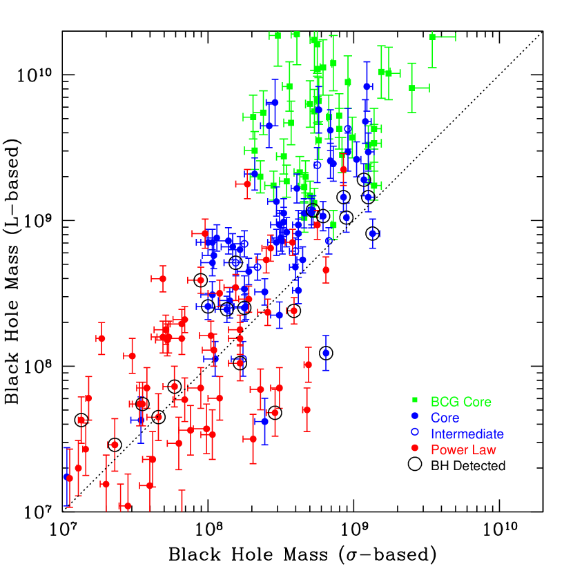
Figure 2: $M_{\bullet}(L)$ versus $M_{\bullet}(\sigma)$ the sample galaxies that have $\sigma$ measurements. Power-law galaxies are plotted as red dots, core galaxies are blue dots, “intermediate” galaxies are plotted as small open circles, and BCGs with resolved cores are plotted as green squares. Galaxies with large circles have directly determined black hole masses; however, the predicted rather than observed $M_{\bullet}$ values are still plotted. The $M_{\bullet}-\sigma$ relationship is that of Tremaine et al. (2002). The asymmetric error bar in the horizontal direction shows the change in predicted $M_{\bullet}$ if the (Wyithe, 2006) log-quadratic $M_{\bullet}-\sigma$ relationship is used instead. $M_{\bullet}(L)$ is the average of the minimum and maximum predictions for a given $L$ from the three $M_{\bullet}-L$ relationships in Figure 1, with the error bars showing the range of the predictions.

Figure 2 shows $M_{\bullet}(L)$ based on a combination of the three relationships presented in Figure 1 plotted against $M_{\bullet}(\sigma)$ from equation (1) for the sample. The error bars along the $M_{\bullet}(L)$ axis reflect the minimum and maximum predictions of $M_{\bullet}$ given by the three relationships shown in Figure 1; the central values plotted are the mean of the minimum and maximum predicted $M_{\bullet}.$ The $L$ and $\sigma$ predictors diverge at large $L,$ with all three $M_{\bullet}-L$ relationships predicting $M_{\bullet}\sim 10^{10}M_{\odot}$ for the most luminous galaxies, while equation (1) predicts no values of $M_{\bullet}$ larger than $\sim 3\times 10^{9}M_{\odot}.$ The errors in $M_{\bullet}(L)$ increase somewhat with galaxy luminosity but are much smaller than the differences between $M_{\bullet}(L)$ and $M_{\bullet}(\sigma),$ which approach an order of magnitude for some of the most luminous galaxies.

The differences between $M_{\bullet}(L)$ and $M_{\bullet}(\sigma)$ cannot be reconciled by the Wyithe (2006) log-quadratic $M_{\bullet}-\sigma$ relationship. The asymmetric error bars in the $\sigma$-based predictions of $M_{\bullet}$ shown in Figure 2 reflect the implied change in predicted $M_{\bullet}$ if the Wyithe (2006) relationship is used instead of the Tremaine et al. (2002) log-linear $M_{\bullet}-\sigma$ relationship. The Wyithe (2006) relationship predicts slightly larger $M_{\bullet}$ only for the largest $\sigma$ values ($\sim 30\%$), but still does not match the even larger $M_{\bullet}(L)$ for the same galaxies. As expected, $M_{\bullet}(L)$ and $M_{\bullet}(\sigma)$ do agree on average for the sample galaxies that actually have direct $M_{\bullet}$ determinations, since it was this subset of galaxies that defined the relationships in the first place.

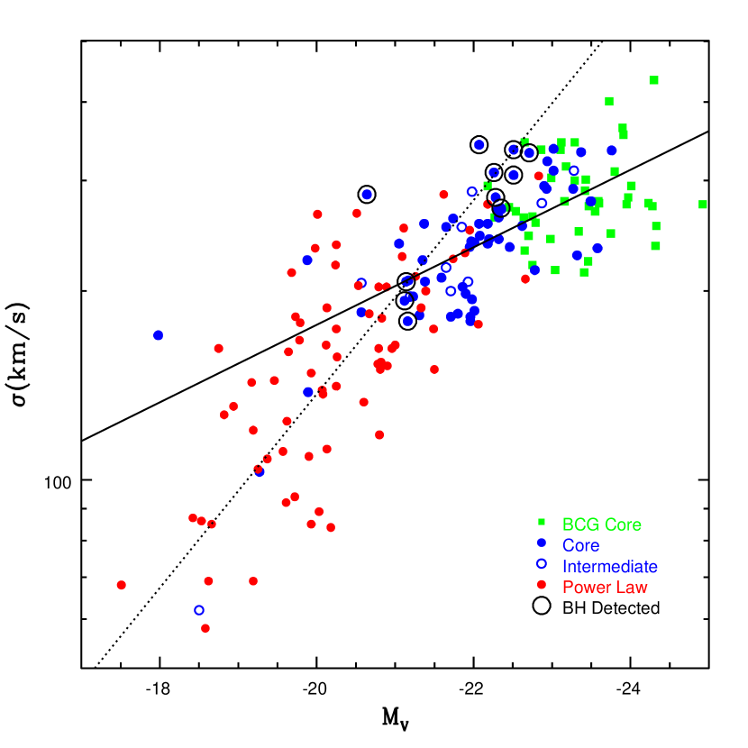
Figure 3: The relationship between central velocity dispersion, $\sigma,$ and $L$ for the sample is plotted. A fit to just the core galaxies and BCGs (solid line; equation 5) gives $L\sim\sigma^{7},$ a much steep relationship then the standard $L\sim\sigma^{4}$ Faber-Jackson relationship, and $L\sim\sigma^{2}$ for the power-law galaxies alone (dashed line; equation 6). It is this change in slope that leads to conflicting predictions for $M_{\bullet}$ from the $M_{\bullet}-L$ and $M_{\bullet}-\sigma$ relation for the most luminous galaxies. Core galaxies with directly measured black hole masses are circled.

The disagreement of the two $M_{\bullet}$ predictors for the larger set of galaxies lacking direct $M_{\bullet}$ determinations can be traced to changes in the form of the $L-\sigma$ relationship as a function of galaxy luminosity. Figure 3 shows this relationship for the sample galaxies. The typical $\sigma$ value appears to level off for large $L$; indeed, there appears to be little relationship between $\sigma$ and $L$ for galaxies with $M_{V}<-22.$ While most of the galaxies in this luminosity range are BCGs, other bright ellipticals show the same behavior. Put simply, the high luminosities of BCGs and other similarly bright ellipticals are not matched by similarly large velocity dispersions. The $M_{\bullet}-\sigma$ relationship thus predicts unexceptional black hole masses for these exceptionally luminous galaxies.

This “saturation” in $\sigma$ at BCG luminosities was noted in the BCG velocity dispersion study of Oegerle & Hoessel (1991), but it appears only weakly in the SDSS study of Bernardi et al. (2003). We suggest that this may be due to the use of different BCG luminosities, based on the analysis of the SDSS magnitudes of BCGs presented in Appendix A. For the core galaxies, we find $L\sim\sigma^{7},$ a much steeper relationship than the classic $L\sim\sigma^{4}.$ Specifically, a symmetrical least-squares fit (Press et al., 1992) to the 99 core galaxies with $M_{V}<-21$ and having a $\sigma$ value produces:

$$M_{V}=-2.5~{}(6.5\pm 1.3)\log(\sigma/{\rm 250~{}km~{}s^{-1}})-22.45\pm 0.18.$$ (5)

However, since the $L-\sigma$ relationship appears to be nonlinear, even this fit may not be the best approximation for the most luminous galaxies. This result also contrasts with the relationship measured for power-law galaxies alone,

$$M_{V}=-2.5~{}(2.6\pm 0.3)\log(\sigma/{\rm 150~{}km~{}s^{-1}})-20.30\pm 0.10.$$ (6)

The distribution of points with $M_{\bullet}$ measurements shows what appears to be a bias in the BH sample: galaxies with $M_{V}\sim-22.5$ with measured $M_{\bullet}$ have a higher-than-average $\sigma$ than typical galaxies at this luminosity — or conversely have low luminosities for their $\sigma$ values (see also Bernardi et al. 2006c). The 7 galaxies with measured $M_{\bullet}$ at $M_{V}\sim-22.5$ have average $\sigma=311\pm 25{\rm~{}km~{}s^{-1}},$ while equation (5) predicts only $\sim 250{\rm~{}km~{}s^{-1}}$ at $M_{V}\sim-22.5$ in agreement with the average $\sigma$ at this luminosity for the SDSS sample (Bernardi et al., 2003). If $\sigma$ is the best predictor of $M_{\bullet},$ then the black holes in these galaxies should be on average $(314/250)^{4}\approx 2.4\times$ more massive than is typical for galaxies with $M_{V}\sim-22.5.$ The $M_{\bullet}-L$ relationship in turn would be biased at the high luminosity end, and the large black hole masses predicted from $L$ shown in Figure 2 will be over-estimates. Conversely, if $L$ is the better predictor of $M_{\bullet},$ then then the $M_{\bullet}-\sigma$ relationship would be biased to predict lower $M_{\bullet}$ than would be correct.

The possibility that the galaxies with measured $M_{\bullet}$ are a biased sampling of the $L-\sigma$ relationship is echoed in Figure 2. For $M_{\bullet}>10^{8}M_{\odot},$ $M_{\bullet}(L)$ is on average greater that $M_{\bullet}(\sigma)$ for galaxies in the present sample. Lowering $M_{\bullet}(L)$ by the bias factor inferred above, or increasing $M_{\bullet}(\sigma)$ by a similar factor would bring the average predictions into excellent agreement, however. Note the galaxies with measured $M_{\bullet}$ in Figure 2, are presently in excellent agreement, since these are the very systems used to define the $M_{\bullet}-\sigma$ and $M_{\bullet}-L$ relationships.

Figure 2 also shows, however, that the large $M_{\bullet}(L)$ predicted for the most luminous galaxies still deviate from $M_{\bullet}(\sigma)$ by a much larger factor than this putative bias. The strong curvature in $L-\sigma$ relationship leads to the upward curvature in $M_{\bullet}(L)$ versus $M_{\bullet}(\sigma)$ well in excess of the selection biases implied by Figure 3. Any luminosity-based predictor of $M_{\bullet}$ calibrated for $M_{V}>-22$ would still predict $M_{\bullet}$ in excess of the $M_{\bullet}-\sigma$ relationship for $M_{V}<-22,$ since $\sigma$ for the brightest galaxies does not increase with luminosity.

4 Core Structure as an Independent Witness of $M_{\bullet}$

4.1 The Cusp Radius

Resolving whether $L$ or $\sigma$ is the best predictor for $M_{\bullet}$ for galaxies with $M_{V}<-23$ will only be possible when real $M_{\bullet}$ determinations can be made in this luminosity regime. Lacking this, we can attempt to obtain preliminary information by considering whether the central structure of galaxies may provide an independent witness to $M_{\bullet}.$ We characterize the physical scale of the core by the “cusp radius,” $r_{\gamma},$ which is the radius at which the negative logarithmic-slope of a galaxy’s surface brightness profile reaches a pre-specified value $\gamma^{\prime}.$ This measure of core size was first proposed by Carollo et al. (1997); we will discuss it in detail in Appendix C. The core is also characterized by the cusp brightness, $I_{\gamma},$ the local surface brightness at $r_{\gamma}$ ($\mu_{\gamma}$ is $I_{\gamma}$ expressed in magnitude units). In terms of the Nuker-law parameters, for $\gamma\leq\gamma^{\prime}\leq\beta,$

$$r_{\gamma}\equiv r_{b}\left({\gamma^{\prime}-\gamma\over\beta-\gamma^{\prime}}\right)^{1/\alpha};$$ (7)

$I_{\gamma}$ is then found directly from the fitted Nuker-law,

$$I_{\gamma}=2^{(\beta-\gamma)/\alpha}I_{b}\left({r_{b}\over r_{\gamma}}\right)^{\gamma}\left[1+\left({r_{\gamma}\over r_{b}}\right)^{\alpha}\right]^{(\gamma-\beta)/\alpha}.$$ (8)

Carollo et al. (1997) advocated use of $r_{\gamma}$ with $\gamma^{\prime}=1/2$ as a core scale-parameter. We show in Appendix C that using $r_{\gamma}$ with $\gamma^{\prime}=1/2,$ indeed gives tighter correlations with other galaxy parameters than the choice of $r_{b}$ as a scale parameter. While the Nuker-law $r_{b}$ is still used to calculate $r_{\gamma},$ we no longer use it directly as a measure of core size, in contrast to the analysis presented in Faber et al. (1997). Lastly, we emphasize that since $r_{\gamma}$ is generally well interior to $r_{b}$ it is not meant to describe the actual complete extent of the core; it is just a convenient representative scale.

4.2 Core Structure and Galaxy Parameters

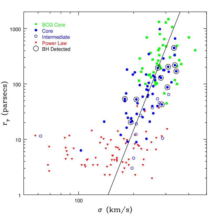
Figure 4: Cusp radius, $r_{\gamma},$ is plotted as a function of stellar velocity dispersion. The power-law galaxies are now plotted as triangles to indicate that their cusp radii are only upper limits. The solid line is the fitted relationship (equation 9) between $r_{\gamma}$ and $\sigma$ for core galaxies. The figure shows that $r_{\gamma}$ is a steep function of $\sigma.$ If $M_{\bullet}\sim\sigma^{4}$ as equation (1), the observed empirical relationship between $r_{\gamma}$ and $\sigma$ (solid line) implies that $r_{\gamma}\sim M_{\bullet}^{2.1\pm 0.4}.$

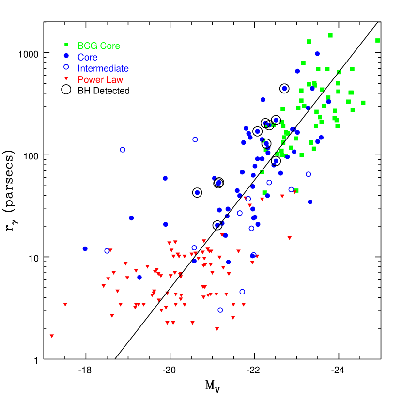
Figure 5: Cusp radius, $r_{\gamma},$ is plotted as a function of total galaxy luminosity. Power-law galaxies are plotted as $\nabla$ to indicate that their $r_{\gamma}$ values are as upper limits. The solid line shows the best-fit relationship between $r_{\gamma}$ and $M_{V}$ for core galaxies (equation 10). The figure shows that $r_{\gamma}$ varies nearly linearly with $L.$ If $M_{\bullet}\sim L_{V}^{1.4}$ as in equation (4), the observed empirical relationship between $r_{\gamma}$ and $L$ (solid line) implies that $r_{\gamma}\sim M_{\bullet}^{0.96\pm 0.09}.$

It has long been known that the physical scale of cores in early-type galaxies is correlated with galaxy luminosity (Lauer, 1985; Kormendy, 1985). This relationship may be due to the action of central black holes on the central distribution of stars (e.g., Faber et al. 1997). Figures 4 and 5 show the relationships between $\sigma,$ $L,$ and cusp radius, $r_{\gamma},$ for the present sample. The $r_{\gamma}-\sigma$ relationship is particularly steep, as $r_{\gamma}$ varies by over two orders of magnitude, while $\sigma$ changes by only a factor of two. For core galaxies with $M_{V}<-21,$ a symmetrical least-squares fit gives

$$\log(r_{\gamma}/{\rm pc})=(8.4\pm 1.6)\log(\sigma/{\rm 250~{}km~{}s^{-1}})+1.99\pm 0.09,$$ (9)

while the $r_{\gamma}-L$ relationship is

$$\log(r_{\gamma}/{\rm pc})=(1.32\pm 0.11)(-M_{V}-23)/2.5+2.28\pm 0.04.$$ (10)

Of the two relationships, $L$ is the better predictor of $r_{\gamma},$ with only 0.31 rms scatter in $\log r_{\gamma},$ while the scatter of $\log r_{\gamma}$ versus $\sigma$ is 0.63. Note that BCGs and non-BCG core galaxies appear to follow the same relationships between $r_{\gamma}$ and $\sigma$ or $L.$ For the non-BCG core galaxies,

$$\log(r_{\gamma}/{\rm pc})=(7.4\pm 1.2)\log(\sigma/{\rm 250~{}km~{}s^{-1}})+2.00\pm 0.07,$$ (11)

and

$$\log(r_{\gamma}/{\rm pc})=(1.94\pm 0.29)(-M_{V}-22)/2.5+1.77\pm 0.06,$$ (12)

while for the BCGs,

$$\log(r_{\gamma}/{\rm pc})=(15.2\pm 7.5)\log(\sigma/{\rm 300~{}km~{}s^{-1}})+2.80\pm 0.31,$$ (13)

and

$$\log(r_{\gamma}/{\rm pc})=(1.24\pm 0.17)(-M_{V}-23)/2.5+2.28\pm 0.05.$$ (14)

While the slopes of the relationships are different from those for the entire sample of core galaxies, there is no significant difference between the relationships within the parameter ranges in which BCGs and non BCGs overlap. A critical result that is evident in Figure 5 is that while BCGs have larger cores than less luminous core galaxies, they are completely consistent with the larger total luminosity of BCGs. In contrast, there is essentially no correlation between $r_{\gamma}$ and $\sigma$ for $r_{\gamma}>300$ pc, as is evident in Figure 4; luminosity is a much better predictor of core size in BCGs than $\sigma.$

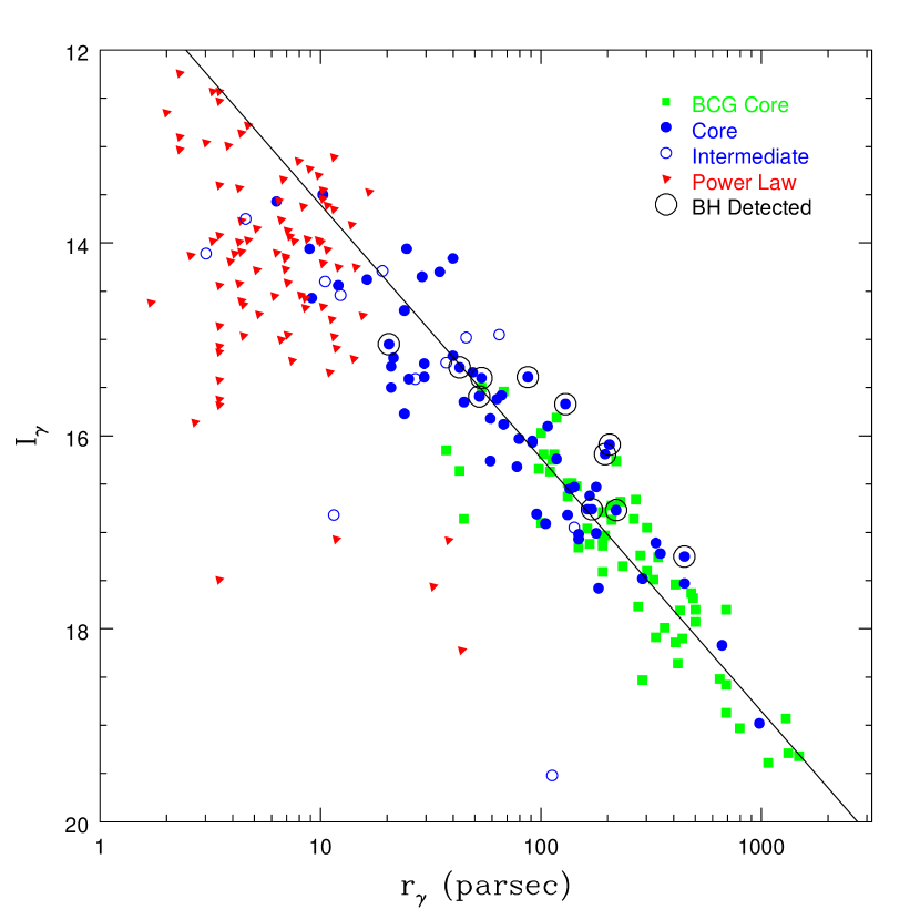
Figure 6: Cusp brightness, $\mu_{\gamma},$ is plotted as a function of cusp radius, $r_{\gamma}.$ The power-law triangles are rotated and shown as arrows to reflect that the points are only upper limits for both $I_{\gamma}$ and $r_{\gamma}.$ The tight relationship between $I_{\gamma}$ and $r_{\gamma}$ (equation 15) means that either can serve for the other in the context of relating core structure to $M_{\bullet},$ $L$ or $\sigma.$

The core is characterized by a surface brightness as well as a physical scale, thus one could also explore the relationships between $I_{\gamma}$ and $\sigma$ or $L,$ but as we show in Figure 6, $I_{\gamma}$ and $r_{\gamma}$ are so closely related that they can be regarded as interchangeable. The fitted relationship between the two parameters for core galaxies with $M_{V}<-21$ is

$$\mu_{\gamma}=2.5~{}(1.05\pm 0.07)\log(r_{\gamma}/{\rm 100~{}pc})+16.23\pm 0.10,$$ (15)

where $\mu_{\gamma}$ is $I_{\gamma}$ in units of $V-$band magnitudes per square-arcsecond.

Lastly, $I_{\gamma}$ and $r_{\gamma}$ can be combined to estimate the stellar mass of the core interior to the cusp as $M_{\gamma}=\pi I_{\gamma}r_{\gamma}^{2}(M/L_{V}),$ again using the conversion between mass and light given in the context of equation (4). Symmetrical fits give the relationships between $M_{\gamma}$ and $L$ or $\sigma$ as;

$$\log(M_{\gamma}/M_{\odot})=(1.35\pm 0.13)(-M_{V}-22)/2.5+9.17\pm 0.05,$$ (16)

and

$$\log(M_{\gamma}/M_{\odot})=(8.6\pm 1.0)\log(\sigma/200{\rm km~{}s^{-1}})+8.55\pm 0.13.$$ (17)

4.3 Core Scouring and Black Hole Mass

4.3.1 Black Hole Mass and $r_{\gamma}$

The existence of the $r_{\gamma}-\sigma$ and $r_{\gamma}-L$ relationships implies empirical relationships between $r_{\gamma}$ and $M_{\bullet},$ given the separate $M_{\bullet}-\sigma$ and $M_{\bullet}-L$ relationships. By combining equation (1) with equation (9) we find $r_{\gamma}\sim M_{\bullet}^{2.1\pm 0.4},$ or more precisely,

$$M_{\bullet}(\sigma)\Longrightarrow\quad\log(r_{\gamma}/{\rm pc})=(2.1\pm 0.4)\log(M_{\bullet}/10^{9}M_{\odot})+2.7\pm 0.2.$$ (18)

At the same time, we can also combine equations (10) and (4) to find $r_{\gamma}\sim M_{\bullet}^{1.0\pm 0.1},$ or

$$M_{\bullet}(L)\Longrightarrow\quad\log(r_{\gamma}/{\rm pc})=(0.96\pm 0.09)\log(M_{\bullet}/10^{9}M_{\odot})+1.9\pm 0.1.$$ (19)

Equations (18) and (19) are inconsistent. The conflict between $M_{\bullet}(L)$ and $M_{\bullet}(\sigma)$ leads in turn to contradictory predictions for how the physical scale of cores is related to black hole mass.

Comparison of the observed $r_{\gamma}-M_{\bullet}$ relationship to the two inferred relationships presented above may offer a path to determining which of $M_{\bullet}(\sigma)$ or $M_{\bullet}(L)$ is more accurate for the most massive galaxies. In the “core-scouring” scenario, cores are created by the orbital decay of a massive binary black hole, which would be formed during the merging of two galaxies. As the merger progresses, black holes in the nuclei of the progenitor galaxies are brought to the center of the merged system by dynamical friction. While the center of the merger may initially be highly concentrated (Milosavljević & Merritt, 2001), as is the case for power-law galaxies, central stars interacting with the binary black hole are ejected from the center as the binary hardens. The ejection of stars erodes the steep central stellar density profile, creating a shallow cusp, or break from the steeper profile that still persists at larger radii. A core is the region of the galaxy interior to the break (cf. Lauer et al. 1995).

Under this hypothesis, the relationship between core scale and $M_{\bullet}$ ought to be more fundamental than either of the $r_{\gamma}-\sigma$ or $r_{\gamma}-L$ relationships alone. The action of the black hole mass on stellar orbits at the galaxy center creates the core structure directly, and the $r_{\gamma}-\sigma$ and $r_{\gamma}-L$ relationships are then merely consequences of the separate $M_{\bullet}-\sigma$ and $M_{\bullet}-L$ relationships. According to this logic, we would conclude that the larger cores of BCGs are evidence of higher BH masses.

A major caveat standing in the way of this conclusion is that core scouring may not lead directly to a clean relationship between $r_{\gamma}$ and $M_{\bullet}.$ The binary BH ejects a total mass of stars, $M_{ej},$ that is expected to be proportional to the total merged $M_{\bullet}$ (Quinlan, 1996; Milosavljević & Merritt, 2001; Merritt, 2006). However, the resultant $r_{\gamma}$ would depend on the radii over which stars are ejected from the center. Further, Merritt (2006) presents simulations that show that core formation should be a cumulative process. Cores formed in one merger event will be depleted even further in subsequent mergers, presumably leading to even larger increases in $r_{\gamma}$ that would reflect not only the total BH mass, but the integrated merger history as well. Under this hypothesis, cores resulting from successive dry mergers would be abnormally large compared to their BH masses, potentially explaining the extra-large cores of BCGs, which are thought to be formed by such multiple mergers. Under scrutiny, however, this explanation seems difficult to support, since the cores of BCGs show no excess compared to the luminosities of their host galaxies, and it is this latter quantity that is probably the best indicator of the amount of dry merging that any massive elliptical has experienced. In other words, the core masses of BCGs galaxies are the same fixed fraction of their total light as in other galaxies, not some amplified value driven by multiple mergers. Thus, we seem to be driven back to the basic explanation that the larger cores of BCGs are due simply to larger BH masses.

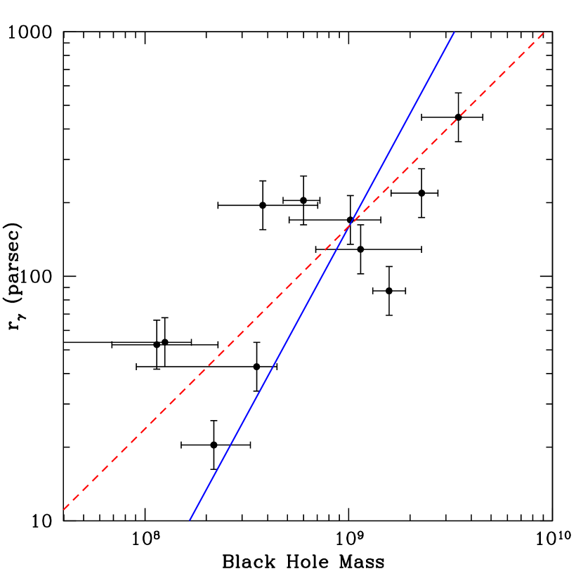
Figure 7: Black hole mass versus core size, $r_{\gamma},$ for the 11 core galaxies that have $M_{\bullet}$ measurements. The red line is the symmetric fit between $M_{\bullet}$ and $r_{\gamma}$ provided by equation (20), while the blue line gives the fit presented in equation (21), which assumes that $r_{\gamma}$ is the independent variable.

Can we use actual core data to identify the correct $r_{\gamma}-M_{\bullet}$ relationship? Figure 7 tries this by plotting $r_{\gamma}$ versus $M_{\bullet}$ for the 11 core galaxies for which there are direct determinations of $M_{\bullet}.$ A symmetric fit to $r_{\gamma}$ and $M_{\bullet}$ for these galaxies has the form

$$\log(r_{\gamma}/{\rm pc})=(0.83\pm 0.25)\log(M_{\bullet}/10^{9}M_{\odot})+2.20\pm 0.10.$$ (20)

This equation is essentially consistent with equation (19), the relationship inferred from $M_{\bullet}(L),$ rather than equation (18), which inferred from $M_{\bullet}(\sigma).$ At the same time, the scatter in Figure 7 is large, thus this result is sensitive to how the $r_{\gamma}-M_{\bullet}$ relationship is fitted. For example, if $r_{\gamma}$ is treated as the independent variable in an attempt to predict $M_{\bullet},$ given $r_{\gamma},$ then

$$\log(r_{\gamma}/{\rm pc})=(1.5\pm 0.8)\log(M_{\bullet}/10^{9}M_{\odot})+2.20\pm 0.11$$ (21)

(although we express $r_{\gamma}$ as the dependent variable for comparison with the relationships above). The slope of this relationship is intermediate between that in equations (18) and (19). For completeness, if $M_{\bullet}$ is treated as the independent variable, which corresponds to the scouring hypothesis that $M_{\bullet}$ determines $r_{\gamma},$ then

$$\log(r_{\gamma}/{\rm pc})=(0.59\pm 0.18)\log(M_{\bullet}/10^{9}M_{\odot})+2.19\pm 0.10$$ (22)

These three fits do not in fact suffice to identify the “correct” $r_{\gamma}-M_{\bullet}$ relation for four reasons: 1) the various slopes differ considerably because the native scatter in the data is large; 2) we are seeking the “true” underlying relationship (i.e., the “theorist’s” question of Novak et al. 2006), but without a knowledge of cosmic scatter and its separate contribution to both $M_{\bullet}$ and $r_{\gamma},$ we cannot fit the data properly to find it; 3) the slopes in equations (18) and (19) were likewise meant to embody “true” relations, but they were derived from prior fits that themselves suffered a similar ambiguity; and 4) the sample of core galaxies with measured $M_{\bullet}$ is potentially biased in some way that is not understood (cf. Figures 3 to 6), and any new fit based on these galaxies might therefore not be representative. On this last point, we emphasize caution. While the galaxies with measured $M_{\bullet}$ may on average have offsets in the parameter plots shown, this does not mean a priori that the directly observed $r_{\gamma}-M_{\bullet}$ relationship is biased. The small number of core galaxies with measured $M_{\bullet}$ plus the number of parameters in play means that understanding any biases must await a richer sample.

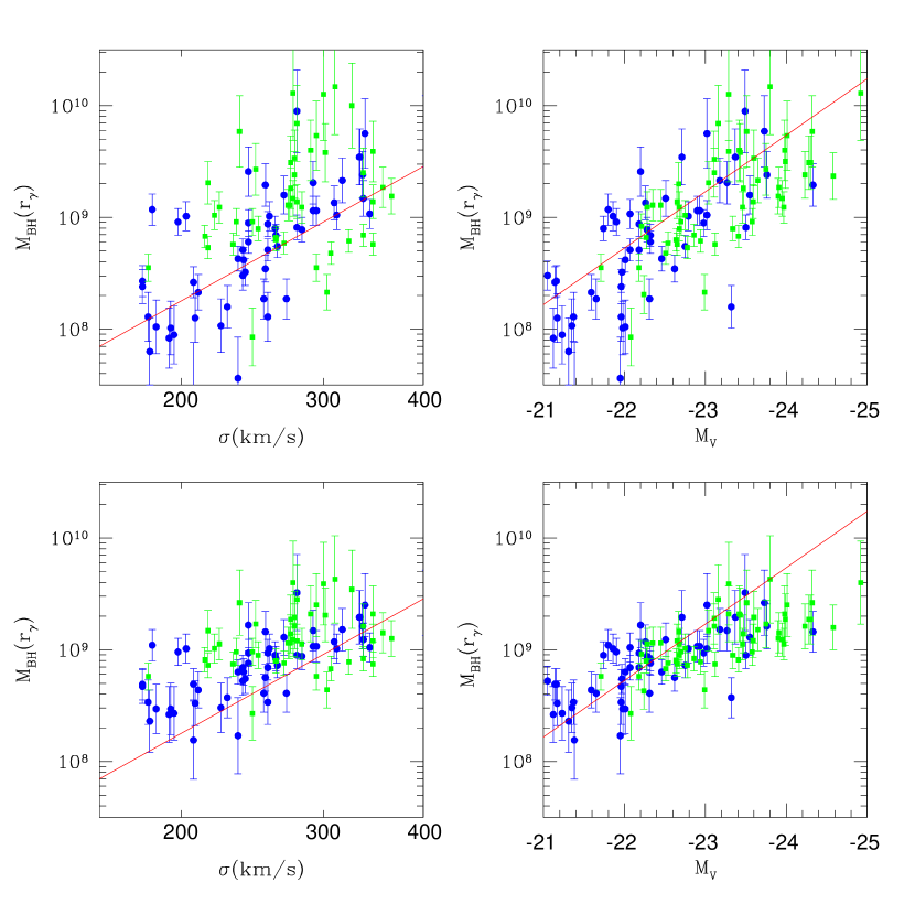
Figure 8: The four panels plot $M_{\bullet}$ predicted from $r_{\gamma}$ as function of $\sigma$ and $M_{V}$ for core galaxies, where green symbols are BCGs, and blue symbols are the remaining core galaxies. The red lines give $M_{\bullet}$ values predicted either from the $M_{\bullet}-\sigma$ relationship (equation 1) or the $M_{\bullet}-L$ relationship (equation 4). The upper panels give $M_{\bullet}$ predicted by $r_{\gamma}$ through equation (20), which was derived by a symmetrical fit to the points in Figure 7. The bottom panels, in contrast, use equation (21), which was derived assuming $r_{\gamma}$ as the independent variable. Both equations typically predict $M_{\bullet}$ in excess of the predictions from the $M_{\bullet}-\sigma$ relationship.

Likewise, the sample of core galaxies with measured $M_{\bullet}$ will have to be increased considerably before it can be used to convincingly discriminate between the $M_{\bullet}(L)$ and $M_{\bullet}(\sigma)$ relations. Nevertheless, we may be able to obtain some guidance in advance of such observations by comparing $M_{\bullet}$ estimated from $r_{\gamma}$ to values estimated from $L$ or $\sigma.$ Figure 8 shows the results of using either equation (20) or (21) to predict $M_{\bullet}$ from $r_{\gamma},$ in analogy to Figure 2, which compared predictions of $M_{\bullet}$ based on $\sigma$ versus $L.$ Both versions of the $r_{\gamma}-M_{\bullet}$ relationship predict larger $M_{\bullet}$ than would be inferred from $M_{\bullet}(\sigma).$ The symmetrically-fitted $r_{\gamma}-M_{\bullet}$ in equation (20) appears to be consistent with $M_{\bullet}(L),$ also predicting $M_{\bullet}\sim 10^{10}M_{\odot}$ for the most massive galaxies.

Presently, the large scatter in the observed $r_{\gamma}-M_{\bullet}$ relationship and the attendant uncertainties in any empirical relationship derived from it does not decisively favor $M_{\bullet}(L)$ over $M_{\bullet}(\sigma).$ Equations (20) and (21) however, on average predict greater $M_{\bullet}$ than would be inferred from $M_{\bullet}(\sigma),$ while equation (20) is consistent with the larger black hole masses implied by $L$ for the most massive galaxies. At this early stage the $r_{\gamma}-M_{\bullet}$ relationship thus may favor consistency with the $M_{\bullet}(L)$ relationship. The fact that the scatter of $r_{\gamma}$ on $L$ is smaller than that on $\sigma$ (as would be expected if $r_{\gamma}$ is produced directly by black hole scouring and $M_{\bullet}$ correlates more closely with $L$) as well as the fact that $M_{\bullet}(L)$ plausibly explains the large core of BCGs as being due to more massive black holes, whereas $M_{\bullet}(\sigma)$ seems to provide no ready explanation this, may offer additional support that $M_{\bullet}(L)$ is more appropriate for the most massive galaxies.

4.3.2 Black Hole Mass and Core Mass

An alternative approach to explore the relationship between core structure and black hole mass is to compare the core mass, $M_{\gamma}=\pi I_{\gamma}r_{\gamma}^{2}(M/L_{V})$, rather than $r_{\gamma},$ to $M_{\bullet}.$ Although, as we noted earlier, $I_{\gamma}$ and $r_{\gamma}$ are closely related, so the relationship between $M_{\gamma}$ and $M_{\bullet}$ will contain information similar to the $r_{\gamma}-M_{\bullet}$ relationship, core mass should be a more direct indicator of the amount of core scouring and its relationship to black hole mass. If cores are created from power-law galaxies by core scouring following a dry merger, one might expect that the core mass would be approximately proportional to the black-hole mass. This conjecture is supported by N-body calculations by Merritt (2006), who argues that the core mass produced by scouring in a single merger is $\simeq fM_{\bullet}$, where $M_{\bullet}$ is the mass of the merged black hole and $f\simeq 0.5$, largely independent of the mass ratio of the merging black holes; he also argues that the total core mass after $N$ dry mergers should be given by $f\simeq 0.5N$. Direct estimation of the mass ejected from the core by scouring is much more difficult observationally than theoretically, because we do not know the state of the galaxy before the merger. Thus we will simply use $M_{\gamma}$ as an “indicative” core mass, recognizing that the factor $f$ relating indicative core mass to black-hole mass is very uncertain, but should be approximately independent of galaxy luminosity for core galaxies.

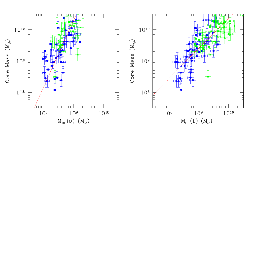
Figure 9: The two panels plot core mass $M_{\gamma}$ as function of $M_{\bullet}(\sigma)$ and $M_{\bullet}(L)$ for core galaxies, where green symbols are BCGs, and blue symbols are the remaining core galaxies. The red lines give the mean $M_{\gamma}-M_{\bullet}$ relationships inferred by combining either the $M_{\bullet}-\sigma$ relationship (equation 1) with the $M_{\gamma}-\sigma$ (equation 17), or the $M_{\bullet}-L$ relationship (equation 4) with the $M_{\gamma}-L$ relationship (equation 16).

Figure 9 shows the relationships between $M_{\gamma}$ and $M_{\bullet}$ as derived from the $M_{\bullet}-\sigma$ and $M_{\bullet}-L$ relationships. By combining $M_{\bullet}(\sigma)$ (equation 1) with the $M_{\gamma}-\sigma$ relationship (equation 17), we find

$$M_{\bullet}(\sigma)\Longrightarrow\quad\log(M_{\gamma}/M_{\odot})=(2.2\pm 0.3)\log(M_{\bullet}/10^{9}M_{\odot})+10.29\pm 0.18,$$ (23)

while the combinations of $M_{\bullet}(L)$ (equation 4) with the $M_{\gamma}-L$ relationship (equation 16) gives

$$M_{\bullet}(L)\Longrightarrow\quad\log(M_{\gamma}/M_{\odot})=(1.0\pm 0.1)\log(M_{\bullet}/10^{9}M_{\odot})+9.39\pm 0.11.$$ (24)

The relation between indicative core mass and black-hole mass predicted by the $M_{\bullet}-L$ relation is essentially linear, as expected, while the relation predicted by the $M_{\bullet}-\sigma$ relation is twice as steep. Moreover the ratio of indicative core mass to black-hole mass is $\sim 2.4$ at $M_{\bullet}=10^{9}M_{\odot}$ from the $M_{\bullet}-L$ relation, not far from the value of order unity that we might expect, while the corresponding value from the $M_{\bullet}-\sigma$ relation is $\sim 19$. It is difficult to devise dynamical models in which core scouring could be efficient enough to create cores with mass so much bigger than the black-hole mass.

5 The Growth of the Most Massive Galaxies and Why $M_{\bullet}(L)$ Might be Favored Over $M_{\bullet}(\sigma)$

Having found suggestive but not conclusive arguments to prefer one relation over the other, we turn now to physical arguments for additional guidance. We stress again that the tension between $M_{\bullet}(L)$ and $M_{\bullet}(\sigma)$ arises due to the breakdown, or curvature, in the $L-\sigma$ relationship at high galaxy masses. It is appropriate to inquire at least briefly into physical reasons why this might happen, and whether this offers insight into which of $M_{\bullet}(L)$ and $M_{\bullet}(\sigma)$ might be preferred for the most massive galaxies.

Curvature in a gravitational scaling relation may signal a breakdown in perfect homology in galaxy formation, which in turn may reflect a change in the relative importance of different physical processes as a function of galaxy size. One such effect, suggested some time ago, is an increase in the importance of dissipationless (i.e., “dry”) merging in forming the most massive ellipticals (Bender et al., 1992; Faber et al., 1997; Naab et al., 2006). A second effect, following logically from the first, is a change in the nature of dissipationless mergers with galaxy mass. As hierarchical clustering proceeds, clusters of galaxies become more massive, and previously formed elliptical galaxies at the centers of these clusters merge. Each new round of merging thus increases the galaxy stellar mass along with the cluster dark halo mass in which it is embedded. The largest ellipticals are thus produced by dry mergers at the centers of the largest clusters. These are BCGs. The above scenario is supported by the steep environmental dependence among bright ellipticals, the brightest ones being found in the densest environments (Hogg et al., 2004).

There are at least two trends that might contribute to a breakdown in perfect homology for dry merging to produce the observed curvature in the $L-\sigma$ relationship. The first is a change in the typical orbital eccentricity of central merging pairs as cluster mass grows. Boylan-Kolchin et al. (2006) have suggested that head-on collisions may become more frequent when massive clusters merge, and their N-body simulations indicate less loss of energy from stars to dark matter in such collisions. The resultant stellar remnants are puffed up in radius and have significantly lower stellar velocity dispersions compared to encounters with normal orbital geometry. A second effect, not considered by them, is the fact that the ratio of cluster velocity dispersion to internal galaxy velocity dispersion also rises as clustering proceeds. This appears to happen because gas cooling is reduced in large dark-matter halos (e.g., Birnboim & Dekel 2003), which means that the baryonic masses of central galaxies grow more slowly than their dark-matter halos. This is why the stellar velocity dispersions within BCG galaxies in large clusters are so much lower than those of their surrounding clusters, whereas the same is not true of ellipticals in small groups (cf. Figure 2 of Blumenthal et al. 1984). The net result is that central merging pairs will approach each other at relatively higher speeds, with the potential of injecting more orbital kinetic energy into the final stellar remnant. This would also cause the remnant to puff up and have smaller final velocity dispersion.

The relative importance of these two effects can only be decided using realistic two-component N-body simulations containing both stars and dark matter that are appropriately embedded in a cosmological clustering scenario. It seems probable that both effects will be found to play a role. The point for now is that there are at least two reasons to expect non-homology in dissipationless mergers, and thus two reasons for curvature in the $L-\sigma$ relationship.

If this logic is correct, it points towards $M_{\bullet}(L)$ as being the proper scaling law for massive galaxies. That is because the major growth in black hole mass during dissipationless merging occurs by merging black holes as the galaxies themselves merge. With little mass accretion directly onto black holes during this stage and no attendant star formation, black hole mass should increase in proportion to galaxy mass. The ratio of stellar mass to black hole mass is constant over dry merging, consistent with $M_{\bullet}$ scaling linearly with galaxy mass. Conversely, for $M_{\bullet}(\sigma)$ to be maintained over dry merging, given the plateau in $\sigma$ at high galaxy luminosity, would require one of the two merging black holes to be ejected from the galaxy as a common occurrence. These arguments provide yet a another reason to prefer the $M_{\bullet}(L)$ relation over $M_{\bullet}(\sigma).$

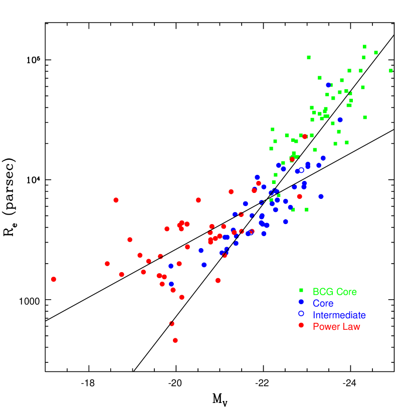
Figure 10: Effective radius as a function of luminosity for the galaxy sample. The steepening of the $R_{e}-L$ relationship sets in at $M_{V}<-22,$ similar to the luminosity at which the velocity dispersion starts to “plateau” in Figure 3. We attribute this to a progressive change in the character of “dry mergers” at higher galaxy masses. The shallow line is defined by a fit to power-law galaxies only (equation 25), while the steep line is a fit to core galaxies with $M_{V}<-21$ (equation 26). Power-law galaxies and core galaxies, however, have similar $R_{e}$ at $M_{V}\sim-21$ where the transition between the two forms takes place.

Regardless of which mechanism is dominant for determining the velocity dispersion of the merged galaxy, “puffing-up” of the remnant does appear to happen in the most luminous galaxies, supporting an overall scenario in which velocity dispersion in the largest galaxies does not increase strongly via mergers. The evidence for this comes from the effective radii of the largest galaxies (see also Bernardi et al. 2006b). Figure 10 shows the $R_{e}-L$ relationship for the whole sample, where $R_{e}$ is the effective radius measured from $r^{1/4}$-law fits to those galaxies that have ground-based surface photometry extending to large radii (Lauer et al., 2007a). For low galaxy luminosity, the the mean $R_{e}-L$ relationship is relatively shallow. We find

$$\log(R_{e}/{\rm pc})=(-0.50\pm 0.08)(M_{V}+21)/2.5+3.62\pm 0.04$$ (25)

based on fits to just power-law galaxies. This stands in contrast to the steeper relationship defined by core galaxies with $M_{V}<-21,$

$$\log(R_{e}/{\rm pc})=(-1.18\pm 0.06)(M_{V}+23)/2.5+4.27\pm 0.02$$ (26)

The transition between the two forms occurs at $M_{V}\approx-22,$ which corresponds to the luminosity at which the average central structure changes from power-law to core (Lauer et al., 2007a). This is also the scale at which $\sigma$ starts to plateau in Figure 3 — the leveling-off of the $L-\sigma$ relationship is thus associated with a rapid increase in $R_{e}$ with $L$ not seen in less luminous galaxies. This is as predicted if extra energy is injected into these galaxies by merging: the objects will have lower $\sigma$ but larger $R_{e}.$

It should be stressed that the arguments presented in support of the $M_{\bullet}(L)$ relation in this section apply only to bright ellipticals, which are those produced by dissipationless merging. The mass-accretion processes that built black holes when galaxies were younger were drastically different and might have obeyed different scaling laws. The $M_{\bullet}(\sigma)$ law might be a better fit to such galaxies, which in general will be smaller than the objects considered in this paper. The broader point of this discussion, however, is that “non-homology” processes may have affected the growth of galaxies generally, with the result that a single black hole scaling law with global galaxy properties might not fit all galaxies.

6 The Space Density of the Most Massive Black Holes

The preceding sections have presented suggestive if not conclusive reasons to suspect that the $M_{\bullet}-L$ relation might be a better predictor of black hole mass than the $M_{\bullet}-\sigma$ relation for the most massive galaxies.

1. The velocity dispersions of the most massive elliptical galaxies rises slowly if at all with galaxy luminosity implying that their black holes are no larger than those of much smaller ellipticals if $M_{\bullet}-\sigma$ is the governing relation — this seems rather surprising.

2. The core-scouring model says that $r_{\gamma}$ should correlate directly with $M_{\bullet}$ whereas correlations between $r_{\gamma}$ and $L$ or $\sigma$ should be secondary; if so, the smaller scatter of $r_{\gamma}$ on $L$ validates $L$ as the more accurate predictor of $M_{\bullet}$.

3. The $M_{\bullet}-L$ relation offers a simple explanation for the large cores of BCGs in terms of bigger black holes whereas the $M_{\bullet}-\sigma$ relation offers no such ready explanation.

4. Either of the two fits of $M_{\bullet}$ on $r_{\gamma}$ for core galaxies with measured BHs (equations 20 and 21) predicts large $M_{\bullet}$ when extrapolated to luminous galaxies, in better agreement with $M_{\bullet}-L$ than with $M_{\bullet}-\sigma$.

5. The largest elliptical galaxies are believed to be formed by dry merging, which predicts that black hole mass should grow in proportion to stellar mass; the observed $M_{\bullet}\propto L$ relation is thus the simplest relation predicted on these grounds. By contrast, the saturation of black holes mass in the largest galaxies that is predicted by the $M_{\bullet}-\sigma$ relation requires that one of the two merging BHs be ejected from the galaxy as a common occurrence, which may not by natural.

6. The largest elliptical galaxies are likely formed by dry mergers at the centers of massive clusters; non-homology merger arguments plausibly explain the low velocity dispersions (and large radii) of such galaxies, but the same arguments then imply that $\sigma$ ought not to be a fundamental parameter for predicting black hole mass in the biggest galaxies.

7. As noted in the introduction, there is evidence from AGN physics that $M_{\bullet}\sim 10^{10}M_{\odot}$ in some systems.

Although these lines of argument are not conclusive, they motivate us to consider the implications for the local BH mass function should the $M_{\bullet}-L$ relation prove correct. The differences from the $M_{\bullet}-\sigma$ relation are large, as we shall show. In this section we first compute these two mass functions based on $M_{\bullet}-\sigma$ and $M_{\bullet}-L$, and then we compare the resulting mass functions to estimates of the relic black hole mass function based on the space density of QSOs as a function of luminosity and redshift.

6.1 The Black Hole Cumulative Mass Distribution Functions

We first compute the black hole mass function by combining the $M_{\bullet}(\sigma)$ predictor with the velocity-dispersion function (the space density of galaxies as a function of velocity dispersion), We then repeat the calculation, but then using $M_{\bullet}(L)$ combined with the galaxy luminosity function. Our analysis follows the precepts of Yu & Tremaine (2002), departing in the choice of dispersion functions. Both calculations use the same formalism, thus for the sake of generality we denote the log of either the velocity dispersion, $\sigma,$ or luminosity of the galaxy, $L,$ by $s$ and assume that the correlations of BH mass $M_{\bullet}$ with either parameter can be formalized through the statement that the probability of finding a galaxy a given BH mass is

$$dP(M_{\bullet})=(2\pi\Delta^{2})^{-1/2}\exp\left[-{[\log(M_{\bullet})-F(s)]^{2}\over 2\Delta^{2}}\right]d\log(M_{\bullet}),$$ (27)

where $F(s)$ is the ridge line of either $\log(M_{\bullet})-s$ relation. The number of BHs near a given mass is then

$${d\,n(M_{\bullet})\over d\log(M_{\bullet})}=(2\pi\Delta^{2})^{-1/2}\int_{-\infty}^{\infty}{dn\over ds}\,\exp\left[-{[\log(M_{\bullet})-F(s)]^{2}\over 2\Delta^{2}}\right]ds,$$ (28)

and the cumulative distribution is

$$n(M_{\bullet})=\int_{M_{\bullet}}^{\infty}{d\,n(M_{\bullet})\over d\log(M_{\bullet})}d\log(M_{\bullet}).$$ (29)

For the dispersion-based predictor, we start with the Sheth et al. (2003) SDSS-based velocity-dispersion function. Bernardi et al. (2006a) reprocessed the SDSS data and recovered a number of galaxies with larger dispersions than those used in Sheth et al. (2003). We use that set of high dispersion galaxies to compute a cumulative dispersion function above $\sigma=350{\rm km~{}s^{-1}}$ by

$$n(>\sigma)=N(>\sigma)/V,$$ (30)

where $N(>\sigma)$ is the number of galaxies with dispersions greater than $\sigma$ and $V$ is the Sloan survey volume given by Bernardi et al. (2006a) as $3.34\times 10^{-7}{\rm Mpc}$ (for $H_{0}=70~{}{\rm km~{}s^{-1}~{}Mpc^{-1}}$ and $z<0.3$). This cumulative function is well approximated by a power law. Differentiating it gives an estimate of the dispersion function above $\sigma=350{\rm km~{}s^{-1}}$ of

$${d\,n(M_{\bullet})\over d\log(\sigma)}=6.67\times 10^{-6}\left({\sigma\over 350{\rm km~{}s^{-1}}}\right)^{-10.27}{\rm Mpc}^{-3}$$ (31)

Equation 31 predicts about 10 times as many galaxies with dispersions greater than $400{\rm km~{}s^{-1}}$ as the Schechter function fit given in Sheth et al. (2003). Above $\sigma=350{\rm km~{}s^{-1}}$ we add it to the Sheth et al. (2003) dispersion function in the analysis of equation (28).

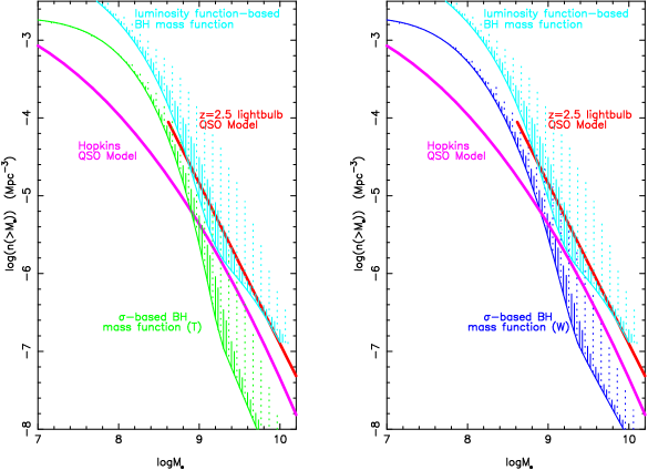
Figure 11: The log cumulative density of black holes above a given mass versus $\log M_{\bullet}$ for different mass functions. The red curve in both panels is derived from a lightbulb model for quasars applied to the Richards et al. (2005) best-fit quasar luminosity function from SDSS, evaluated at $z=2.5$. The model assumes they radiate at their Eddington Luminosity with a duty fraction $f=0.03$ (see text). The pink curve in both panels is the BH mass function produced by the Hopkins et al. (2006) model for quasar, described in detail in the text. The cyan curve in both panels is the BH mass function obtained by augmenting the Blanton et al. (2003) best-fit Schechter (1976) luminosity function for SDSS galaxies with the Postman & Lauer (1995) brightest cluster galaxies and calibrated by the Häring & Rix (2004) relation. The solid and dotted lines above the curve show the effect of cosmic scatter of 0.25 and 0.50 (respectively) about the mean relation (derived by Häring & Rix (2004)) between BH mass and galaxy mass. The green curve (in the left panel) is a BH mass function predicted from the SDSS velocity dispersion function (Sheth et al., 2003) augmented by the Bernardi et al. (2006a) high-dispersion sample and calibrated by the Tremaine et al. (2002) $M_{\bullet}(\sigma)$ predictor for zero cosmic scatter. The solid and dotted lines above the curve show the effect of a cosmic scatter of 0.15 and 0.30 in the decimal log of the BH mass about the mean Tremaine relation. The dark blue curve in the right panel illustrates the same dispersion function calibrated instead by the Wyithe (2006) $M_{\bullet}(\sigma)$ predictor.

We think this is the best available estimate of $dn/dlog(\sigma)$ for early-type galaxies at zero redshift. We combine the Sheth/Bernardi dispersion function with the Tremaine et al. (2002) $M_{\bullet}(\sigma)$ predictor (equation 1) $F(s)=8.19+4.02\times x$ where $x=s-\log(200~{}{\rm km~{}s^{-1}})$, in equations 28 and 29. As an alternative, we consider the $\sigma$ – BH mass function using the Wyithe (2006) predictor $F(s)=8.11+4.2\times x+1.6\times x^{2}$. We illustrate both cumulative BH mass functions so derived in Figure 11. Choosing the Wyithe predictor only increases the predicted BH number density modestly near $M_{\bullet}=3\times 10^{9}M_{\odot}$.

Inclusion of the cosmic scatter in the $M_{\bullet}$ relationships is crucial (Yu & Tremaine, 2002; Yu & Lu, 2004; Tundo et al., 2006). The total population of galaxies at any given $L$ or $\sigma$ will host black holes with a range in $M_{\bullet}.$ The final BH mass functions thus are not a simple “relabeling” of the $L$ or $\sigma$ distributions with black hole mass, but are rather a convolution of the of these distributions with an assumed distribution of $M_{\bullet}$ at constant $L$ or $\sigma.$ This convolution is especially critical at a large BH mass, where both the galaxy luminosity and dispersion functions decline rapidly. As a result of cosmic scatter, most of the high mass BHs actually come from “modest” galaxies with unusually large BHs for their luminosities or dispersions, as compared to the expected contribution of massive black holes from the most massive galaxies (Lauer et al., 2007b).

We emphasize that $\Delta$ above is the scatter about the mean relation due to cosmic scatter in the relation and not due to measurement error. Tremaine et al. (2002) notes that the $\Delta=0.30$ scatter about their derivation of $M_{\bullet}(\sigma)$ might be entirely due to measurement error, leaving no room for cosmic scatter. In plots of BH mass functions in Figure 11 we illustrate illustrate 3 values of the cosmic scatter for the Tremaine and Wyithe results: $\Delta=0,\ 0.15\ {\rm and}\ 0.30$. This scatter is probably not larger than $0.30$, but may be considerably smaller.

We compute the the $L$-based black hole mass function by the same approach, starting with the Blanton et al. (2003) SDSS $g^{\prime}$ galaxy luminosity function. We convert the $g^{\prime}$ galaxy luminosity function to $V-$band using $g^{\prime}=V+0.41$ — suitable for E galaxies at $z=0$ (Fukugita et al., 1995). Comparison of the Blanton et al. galaxy luminosity function with the Postman & Lauer (1995) BCG survey suggests that the Blanton work undercounts BCGs. We argue in Appendix A that this may be due to the effects of excessive sky subtraction on the most luminous galaxies. To correct for this, we have added an estimate of the space density of BCGs as a function of V-band luminosity to the Blanton et al. sample. We used the Postman & Lauer (1995) BCG sample, which is volume-limited, to construct an estimate of the luminosity function in $R_{C},$ transforming it to $V$ using $R_{C}=V-0.55$. Using the combined $dn/dM_{V}$, we determine the number of BHs above a specified mass $M_{\bullet}$ from equations 29 and 28, where we set $s=M_{V}$ and $F(s)$ is the right-hand side of equation (4) — the Häring & Rix (2004) predictor. Because Blanton et al. (2003) represented their luminosity function as that observed at $z=0.1,$ rather than the present epoch, both k-corrections and corrections for evolutionary fading are required. These two terms fortuitously cancel each other: Blanton et al. (2003) show that their sample dims by 0.2 mag in $g^{\prime}$ from $z=0.1$ to the present, while the filter k-correction to transform to $z=0$ is $-0.20$ mag. Lastly, we use $\Delta=0.25$ and 0.50, larger values than were used for $M_{\bullet}(\sigma),$ given the larger scatter in $M_{\bullet}(L).$

The cumulative BH mass functions based on the two different methods are shown in Figure 11. Near BH masses of $10^{8}M_{\odot}$ (luminosities near $L_{*}$) and lower, the $L$-based function overpredicts BH numbers by a factor of two and larger. In part, this is due to the fact that the $L$-based mass function includes galaxies that are disk-dominated, thereby overestimating the numbers and masses of BH at lower masses, since the $L-M_{\bullet}$ relationship is based on bulges and elliptical galaxies. At higher masses this correction is negligible since most galaxies are ellipticals or bulge dominated S0s. There is also the possibility that the $L-M_{\bullet}$ relationship is biased in the sense that the galaxies with black hole mass determinations have larger velocity dispersions than the average values for galaxies of their luminosities (see Figure 1). If so, this would cause the $L$-based mass function in Figure 11 to shift to the left, in better agreement with the $\sigma$-based mass function.

For $M_{\bullet}>10^{9}M_{\odot}$ the $L$ and $\sigma$ mass functions diverge. The $L$ based mass function predicts a local density of the most massive black holes that is about an order of magnitude greater than would be inferred from the $M_{\bullet}-\sigma$ relationship for $M_{\bullet}>2\times 10^{9}M_{\odot}$. This disagreement was foretold in Figure 2 — the present Figure 11 simply recasts the disagreement between $M_{\bullet}-L$ and $M_{\bullet}-\sigma$ in terms of the BH mass function.

6.2 The Black Hole Distribution Function Inferred From QSOs

There are two different approaches that can be used to infer the present BH mass function from quasar counts (specifically from the joint distribution of quasar numbers as a function of redshift and luminosity). One line, started by Sołtan (1982), relies on energy conservation. Under that argument, the energy emitted by the quasars at any redshift propagates through the universe declining in co-moving density due to the redshift of the photons as $(1+z)^{-1}$, and thus behaves exactly like a background. Hence the observed quasar flux translates directly to the total energy emitted given a known redshift distribution of emitters, and further translates into the total mass accreted by black holes, given their radiative efficiency. An alternate approach, started by Small & Blandford (1992), is to assume that all quasars go through a phase in which they accrete at the Eddington limit, followed by a period of slower or intermittent accretion according to a universal model dependent on BH mass and time. This assumption, together with a continuity argument (the number of BHs at a given mass changes only by accretion and merging) permits the recovery, not merely of the local BH density, but also of the local BH mass function. This second approach achieves a more detailed result than the Sołtan argument, but at the expense of additional assumptions.

A third more limited approach, which shares some logic with Small-Blanford, is to assume simply that the BHs of known mass accrete near the Eddington limit for some period and to ignore their fainter growth period — the so called “lightbulb model.” In this model quasars are either on or off. Because the number of luminous quasars in the universe varies strongly with time, the model doesn’t count BHs directly, rather it counts those that are accreting. In what follows, we evaluate the lightbulb model at $z=2.5$ where the top end of the quasar LF is largest. We assume that no BHs above $10^{9}M_{\odot}$ are destroyed by mergers since that time, so the fall-off in the LF is due to a halt in accretion. At earlier times the BH mass function may be evolving. The full-width half maximum of the bright quasar LF is about $10^{9}$ yrs. So our lightbulb model implicitly assumes that every massive BH accretes for $10^{9}f$ yrs, where $f$ is defined as the duty fraction, and then shuts off. This idealization ignores low mass BHs and low-level accretion. Another significant limitation is that the model provides no procedure to identify the mass below which it fails, although that failure is implicit within the assumptions: some of the lower luminosity quasars must be high mass BHs accreting at less than their Eddington limit. A third limitation is that the model is fundamentally inconsistent: the assignment of mass corresponding to a quasar luminosity gives the instantaneous mass of an accreting BH, while the present day mass function depends on its final mass. If the quasar is “on” for less than the Salpeter time (for BH mass to e-fold in Eddington-limited accretion), then the problem is small, but if it is on for much longer than the Salpeter time it is catastrophic: the present BH mass may be much larger than that assigned to the quasar.

Nonetheless, the lightbulb model permits a comparison of the quasar LF with the number density of the most massive BHs in the local universe, with the duty fraction as a free parameter, under the assumption that the brightest objects in the quasar luminosity function are accreting near the Eddington limit. This approach was used by Richstone et al. (1998) to make a crude estimate of the duty fraction of BH accretion. We perform a similar analysis here. We start with the Richards et al. (2005) luminosity function at $z=2.5$, where the bright quasar density is greatest. The Richards et al. (2005) fit reports number densities per magnitude at an AB absolute magnitude at rest-frame $\lambda=$1500Å. We integrate their fitting function from a given luminosity to infinity to get a cumulative number of objects brighter than that luminosity, we apply a bolometric correction of 5 (Marconi et al., 2004), and then we deduce a mass from the Eddington limit. This procedure identifies the number density of BHs greater than a given mass accreting at a given redshift. We compute this cumulative density at redshift $z=2.5$ where the density of bright quasars is greatest. We divide this result by the duty fraction $f.$ We adopt $f=0.03$ based on the extensive work by Steidel et al. (2002) and Adelberger & Steidel (2005). This yields the line labeled “lightbulb” in Figure 11.

An improvement on both the lightbulb approach and the Small-Blandford approach is to use a physical model for the accretionary evolution of the BHs. One such model is the merger-induced accretion model that has been explored in detail by Springel et al. (2005) and Robertson et al. (2006). They simulate the merger of disk+bulge+BH galaxies containing gas using the GADGET code, treating the BH growth by computing the Eddington-limited Bondi accretion rate at their smallest resolution element. They compute the luminosity of the accreting BH from the accretion rate under reasonable assumptions about the radiative efficiency. Their simulations permit the development of a model (Hopkins et al., 2006) that predicts the X-ray background and the zero-redshift BH mass function from the quasar LF. We believe the Hopkins model is a profound advance over simpler analyses. While it might turn out that their model does not correspond in detail to the quasar phenomenon, the approach may have broader utility. We summarize the salient points of their model below.

The Hopkins et al. (2006) simulations exhibit very complex behavior of luminosity as a function of time for a given galaxy merger, but the time spent above a given luminosity turns out to be a universal profile over a wide range of galaxy or merger parameters, provided it is scaled appropriately with the peak luminosity and relic BH mass of the merger. For their simulations, the lifetime near a given bolometric luminosity L can be parametrized as

$$dt/d\log L=t_{Q}^{*}\exp(-L/L_{Q}^{*}),$$ (32)

where the timescale $t_{Q}^{*}$ (a crude quasar lifetime) and luminosity scale $L_{Q}^{*}$ are functions of the peak luminosity $L_{p}$ as follows.

$$L_{Q}^{*}=0.2L_{p},$$ (33)

and

$$t_{Q}^{*}=1.37\left({L_{p}\over 10^{10}L_{\odot}}\right)^{-0.11}{\rm Gyr}.$$ (34)

The final or relic BH mass has a one-to-one correspondence with the peak luminosity given by

$$M_{\bullet}=1.24\left({L_{p}\over 10^{13}L_{\odot}}\right)^{-0.11}\times M_{Edd}(L_{p}),$$ (35)

where $M_{Edd}(L_{p})$ is the mass with an Eddington luminosity of $L_{p}$. An ensemble of objects with the same $L_{p}$ should have a luminosity distribution proportional to the $dt$ in equation 32.

Hopkins et al. (2006) use the model of quasar lifetimes described above together with a log-normal distribution of quasar birth rate per unit time to match the quasar luminosity function. We use their parameterization

$$\dot{n}={\dot{n}_{*}\over\sigma_{*}\sqrt{2\pi}}\ exp\left(-{[\log(L_{p}/L_{*})]^{2}\over 2\sigma_{*}^{2}}\right),$$ (36)

where $\dot{n}$ is the number of quasars born per unit comoving volume per unit time. Hopkins et al. (2006) find a good fit to the X-ray and optical quasar luminosity functions with

$$L_{*}(z)=L_{*}(0)\exp(k\tau),$$ (37)

where $\tau$ is the dimensionless lookback time $\tau=H_{0}\int dt$ and the other parameters are presumed constant. In what follows we use their best fit model with $(\log L_{*},\ k,\ \log\dot{n}_{*},\ \sigma_{*})=$ (9.94, 5.61, -6.29, 0.91), with $L_{*}$ in solar units and $\dot{n}_{*}$ in comoving ${\rm Mpc}^{-3}{\rm Myr}^{-1}$.

We can compute the present day density of quasar relics by integrating the quasar birthrate over time at any specific mass or $L_{p}$. Therefore the cumulative density of BHs above a given mass $M_{\bullet}$ is

$$n(M_{\bullet})=\int_{L_{p}(M_{\bullet})}^{-\infty}\left[\int_{0}^{z_{max}}\dot{n}{dt\over dz}dz\right]d\log L_{p}.$$ (38)

Following Hopkins et al. (2006) we set $z_{max}=3$. We plot the result of equation (38) in Figure 11.

An important feature of the Hopkins model is that owing to the exponential distribution of time above a given luminosity (equation 32) the quasar spends only a fraction of its lifetime accreting near the Eddington rate. For example, a $10^{9}M_{\odot}$ relic BH had a peak luminosity, $L_{p}$ of $3.03\times 10^{13}L_{\odot}$ and spent the time $t_{e}=t_{Q}^{*}\log e\times E_{1}(5/e)=15{\rm Myr}$ above a factor of $1/e$ of $L_{p},$ where $E_{1}(x)=\int_{x}^{\infty}\exp(-u)/u\ du$ is the usual exponential integral. The Hopkins model guarantees that the BH will accrete enough mass, but not too much, over its lifetime.

Figure 11 permits us to compare the lightbulb and Hopkins models with the two relic BH mass functions. The BH mass functions diverge at about $10^{9}M_{\odot}$. The dispersion-based predictors predict considerably fewer BH at above $10^{9}M_{\odot}$ than the luminosity-based predictors. They are not consistent with the lightbulb model; consistency with the Hopkins model is possible with the Wyithe (2006) form of $M_{\bullet}(\sigma),$ but with the assumption of more cosmic scatter in the $M_{\bullet}-\sigma$ relationship than is probably realistic. The luminosity-based mass function is barely consistent with the lightbulb model, but probably overpredicts the AGN density compared to the Hopkins model. We thus cannot make a clear determination between the dispersion-based and luminosity-based BH mass predictors by comparing zero redshift BH demographics to quasar demographics; however, the linear Tremaine et al. (2002) $M_{\bullet}(\sigma)$ relationship is disfavored in all of the present models to explain the QSO population.

An important caveat is that our calculations have neglected the effects of dry merging on the most massive galaxies after the epoch of QSOs. Merging might produce high mass black holes as a relatively recent phenomenon, thereby helping to reconcile the estimates made from $M_{\bullet}(L)$ with the QSO population. Another caveat for both results is the possibility of super-Eddington accretion among the biggest BHs (Begelman, 2006). If common, super-Eddington accretion would make it very hard to make any estimates of the mass function of relic BHs from quasar LFs.

7 Conclusions

The $M_{\bullet}-\sigma$ relationship has come to be the “gold standard” for predicting black hole masses from galaxy properties due to its small scatter and its implications for illuminating the co-formation of galaxies and their nuclear black holes. At first sight, the $M_{\bullet}-L$ relationship might be dismissed as a simple consequence of the Faber-Jackson relationship. With $M_{\bullet}\sim\sigma^{4}$ and $L\sim\sigma^{4},$ one would expect something like $M_{\bullet}\sim L.$ The larger scatter in the $M_{\bullet}-L$ relationship further suggests that the $M_{\bullet}-\sigma$ relationship is really more fundamental. But as galaxy luminosity increases, $\sigma$ levels off and the basic Faber-Jackson relationship does not appear to hold. At BCG luminosities there are no direct measurements of $M_{\bullet}$ and $M_{\bullet}(\sigma)$ versus $M_{\bullet}(L)$ present contradictory extrapolations. The contradiction essentially begs the question, do these exceptionally luminous galaxies have exceptionally massive black holes? The $M_{\bullet}-L$ relationship answers this in the affirmative, while for the $M_{\bullet}-\sigma$ relationship to be correct we must accept the puzzling result that the black holes in BCGs have relatively modest masses. But this question leads to a broader issue, namely. is is there a significant population of black holes with $M_{\bullet}$ approaching $10^{10}M_{\odot}$ in the local universe?

The best way to answer these questions is to attempt to weigh the BHs in BCGs. With the advent of LASER-guided adaptive optics-fed spectrographs on 10m class telescopes, it is now possible to do this. This paper may therefore be premature. However, given the high attention to the $M_{\bullet}-\sigma$ relationship and its implications for galaxy formation, we believe that advancing the implications of $M_{\bullet}-L$ relationship offers an important alternative view that should not be overlooked. Lacking hard measures of $M_{\bullet}$ in the most massive galaxies, we have marshalled a number of less-direct arguments that this hypothesis may be favored for the most luminous galaxies.

The first set of arguments is based on the hypothesis that cores in the most luminous galaxies are created in a “core scouring” process in which a binary BH created in the merger of two galaxies evacuates stars from the center of the newly-merged product. There presently is little observational support for the creation of binary black holes in mergers, but abundant theoretical work shows that realistic cores can be created by binary black holes, and the prevalence of nuclear black holes in galaxies overall strongly argues that such binaries must be created as a natural consequence of mergers. If so, the physical scale of cores, which we have parameterized as $r_{\gamma}$ may be an independent witness of $M_{\bullet},$ and thus use the large cores in BCGs as an indicator of their black hole masses.

Based on central structural parameters derived from HST observations, we find that the large cores in BCGs are commensurate with their high luminosities, while $\sigma$ is a poor predictor of $r_{\gamma}$ for $r_{\gamma}>300$ pc. The scatter in the $r_{\gamma}-L$ relationship is much smaller than that in the $r_{\gamma}-\sigma$ relationship, again implying that $L$ and core scale are more closely related. The observed $r_{\gamma}-M_{\bullet}$ relationship for 11 core galaxies with directly determined black hole masses has large scatter, but appears to be more consistent with the $M_{\bullet}-L$ rather than the $M_{\bullet}-\sigma$ relationship. Lastly. the core masses in BCGs are over an order of magnitude larger than the black hole masses estimated from $M_{\bullet}(\sigma),$ but are only a few times larger than those estimated from $M_{\bullet}(L);$ making such large cores with the smaller $\sigma$-based black hole masses would be a strong challenge for the core-scouring hypothesis of core formation.

The second set of arguments comes from considering theoretical arguments concerning whether or not $L$ rather than $\sigma$ should predict $M_{\bullet}$ in BCGs. The favored origin of BCGs is that they are the remnants of dissipationless purely-stellar mergers of less-luminous elliptical galaxies, augmented by ongoing galactic cannibalism of elliptical galaxies in the rich environments at the center of galaxy clusters. The plateau in the $L-\sigma$ relationship plus but the steeper $L-R_{e}$ relationship at high galaxy luminosity presented here strongly favor this formation scenario. The luminosity of a BCG is the sum of the luminosities of its progenitors. Similarly, setting aside the possible ejection of nuclear black holes in the final stages of a merger, the final nuclear black hole mass should be the sum of the progenitor black holes. Stated more directly, the ratio $M_{\bullet}/L$ should be largely invariant over dissipationless mergers, leading to $M_{\bullet}\sim L$ at the high end of the galaxy LF. In contrast, $\sigma$ appears to be nearly constant over these mergers. In effect, even if a relationship between $M_{\bullet}$ and $\sigma$ were set up in the initial stages of galaxy formation, it might not survive in a dissipationless merging hierarchy.

A final argument comes from attempting to infer the $z=0$ space density of the remnant black holes associated with the most luminous QSOs seen at $z\sim 2.$ As noted in the Introduction, the properties of the broad-line regions in the most luminous QSOs argue that they are powered by black holes with $M_{\bullet}\sim 10^{10}M_{\odot}.$ The heating of the intra-cluster medium in the richest galaxy clusters may also demand that some black holes in BCGs approach this mass. The critical part of this analysis is understanding how to correct the QSO space density for QSO luminosity evolution. The remnant black holes last forever, but the QSOs represent only those BHs made visible during an epoch of high mass-accretion, which presumably lasts only a small fraction of the age of the universe. We used the Hopkins et al. (2006) simulations to estimate the QSO lifetimes. The resulting shape and space density of the bright end of the QSO LF falls between the higher space density of the most massive black holes implied by $M_{\bullet}(L)$ and those implied by $M_{\bullet}(\sigma),$ while the simple “lightbulb” model of QSO duty cycles favors the $M_{\bullet}(L)$ relation. This treatment is sensitive to the assumed amount of cosmic scatter in both $M_{\bullet}$ relationships; however, it appears difficult for the log-linear $M_{\bullet}-\sigma$ relationship to explain the the observed space densities of the most luminous QSOs without assuming that its cosmic scatter is larger than is likely to be the case.

Appendix A The Luminosities of BCGs and Comparison to SDSS Magnitudes

Our analysis depends critically on the accuracy of the absolute luminosities of the brightest galaxies in the sample, such as BCGs. This is underscored by the bright-end disagreements of our $L-\sigma$ relationship and galaxy luminosity function with those based on Sloan Digital Sky Survey (SDSS) data (Bernardi et al. 2003 and Blanton et al. 2003, respectively). We thus describe the derivation of our BCG luminosities, and compare them to magnitudes based on the SDSS for BCGs in common. We conclude that the SDSS BCG magnitudes are strongly affected by sky subtraction errors, causing them to be biassed to significantly fainter values.

The BCGs in the present sample come from the Laine et al. (2002) HST BCG study. This program, in turn, was based on the volume-limited Postman & Lauer (1995) BCG sample, which provides ground-based profiles and aperture photometry. As outlined in $\S\ref{sec:gallum}$, we derive apparent magnitudes of the BCGs by fitting the classic $r^{1/4}$ form to the inner portions of the brightness profiles, where the inner limit of the fit was set to avoid seeing and the outer limit was specified to avoid portions of the profile that appeared to rise above the $r^{1/4}$ fit. Graham et al. (1996) showed that the BCG profiles could be described by single-component Sérsic (1968) forms, but ones that often had index $n>4.$ The apparent magnitudes, which were derived by integrating the $r^{1/4}$-law over radius, thus if anything are underestimates of the total BCG fluxes. An alternative to this procedure would be to integrate the Sérsic forms, however, as is shown in Graham et al. (1996), the Sérsic $R_{e}$ and $n$ values are closely coupled, such that large $n$ is matched with large $R_{e},$ The implied total magnitude strongly diverges as $n$ increases, and must essentially be regarded as unphysical extrapolations because the derived $R_{e}$ is typically well outside the actual radial domain of the surface brightness profile for large $n;$ this is not true for $n=4.$ A contrasting treatment that occurs in much of the literature is based on the presumption that BCG must be completely well described by $r^{1/4}$-laws (in contrast to other giant elliptical galaxies, which also have $n>4$), and that Sérsic $n>4$ is really the signature of an intracluster light component that must be subtracted. We conclude that an unambiguous procedure to derive total BCG luminosity does not presently exist. Our procedure of deriving magnitudes from just the inner portion of the profile that is well described by an $r^{1/4}$-law again should give a sensible lower limit to the total luminosity.

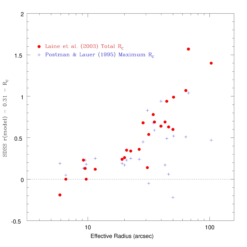
Figure 12: SDSS $r$ “model magnitudes” are compared to two separate $R_{C}$ magnitudes for the Postman & Lauer (1995) BCGs inc common, where the SDSS values are transformed assuming $R_{C}=r-0.31.$ Red points show the difference between SDSS model $r$ magnitudes and the Laine et al. (2002) $R_{C}$ total BCG luminosity versus effective radius, $R_{e},$ which is derived from $r^{1/4}$ fits to the Postman & Lauer (1995) surface brightness profiles. The blue points are the same exercise, but with the Postman & Lauer (1995) maximum-aperture magnitudes used instead. Clearly, the larger a BCG is, the more the present total luminosity disagrees with the SDSS value. The maximum-aperture magnitudes are not intended to be interpreted as a total magnitude, but provide a model-independent lower limit on its value. Since the maximum-aperture magnitudes are brighter than the SDSS magnitudes for most BCGs, this clearly shows that the SDSS values cannot be regarded as total luminosities.

The high luminosity end of the Blanton et al. (2003) luminosity function falls well below the BCG space densities measured by Postman & Lauer (1995). The Bernardi et al. (2003) $L-\sigma$ relationship shows no plateau at its bright limit. These discrepancies would both be explained if the total magnitudes for BCGs in the SDSS database are significantly underestimated. We checked this hypothesis by examining the 25 Postman & Lauer (1995) BCGs present in the SDSS DR4 database. In detail, we compared the total $R_{C}$ apparent magnitude in Laine et al. (2002) against the SDSS $r$ “model magnitude,” (which in almost all cases is the most luminous total magnitude provided by the SDSS database) transformed by $R_{C}=r-0.31.$ The results are shown in Figure 12 as a function of effective radius (based on our fits). A strong systematic trend is evident such that larger galaxies have greater offsets between the two total magnitudes. The median $r-0.31-R_{C}$ value is 0.54 mag and rises to 1.57 mag for the NGC 6166 (the BCG in A2199). As an additional check, we also compared the SDSS $r$ magnitudes against the maximum $R_{C}$ aperture magnitude published by Postman & Lauer (1995). The maximum aperture radius was not defined in any rigorous way and does not correspond to any fixed fraction of the total galaxy flux, but the magnitude is a model-independent integration of all the flux within the published radius. The median difference between the SDSS model $r$ magnitudes (transformed to $R_{C}$) and the maximum aperture magnitude is 0.24 mag and rises to values over a full magnitude for the largest galaxies. This demonstrates directly that the SDSS model magnitudes for the galaxies in question cannot be regarded as total magnitudes.

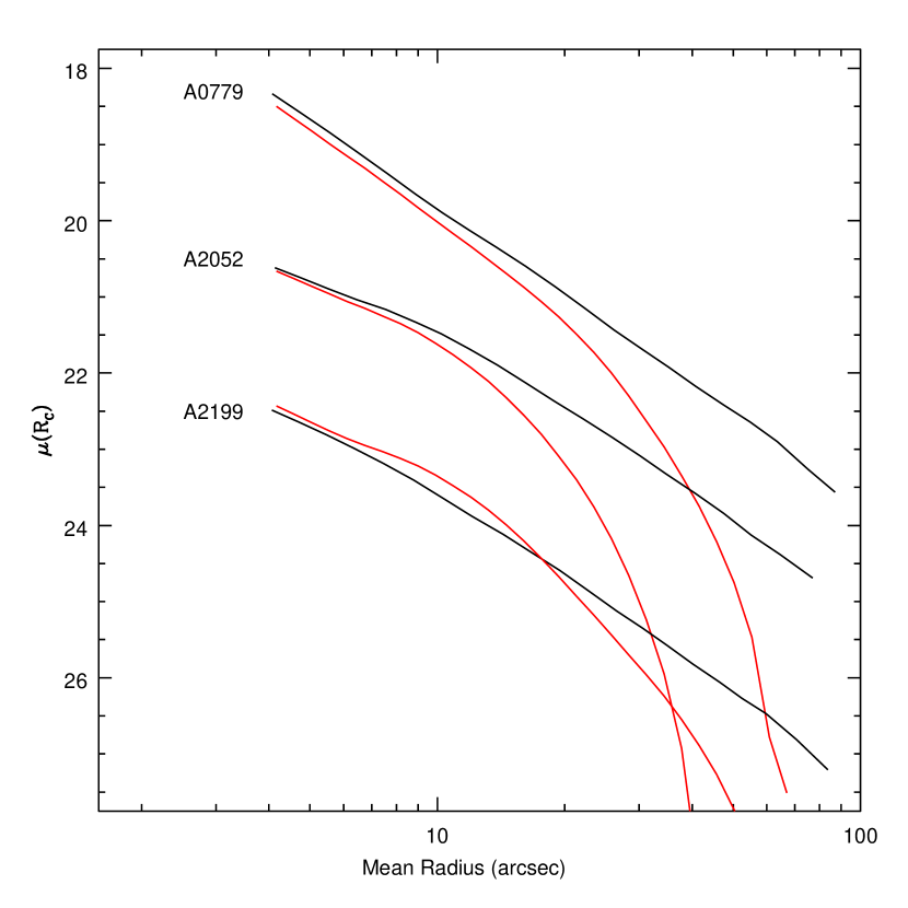
Figure 13: Surface brightness profiles from Postman & Lauer (1995) (black) are compared to “profmean” SDSS profiles (red) for three BCGs. The SDSS $r$ band magnitudes are transformed assuming $R_{C}=r-0.31.$ The SDSS profiles all fall below the Postman & Lauer (1995) profiles at large radii, consistent with excessive sky subtraction by the SDSS pipeline.

Conversations with a number of experienced users of the SDSS database for bright galaxies warned us that the SDSS pipeline measured sky levels on angular scales too small to accommodate bright nearby BCGs of the sort observed by Postman & Lauer (1995), and indeed the results shown in Figure 12 strongly suggest that a sky-subtraction error affects the SDSS magnitudes. As a check, we plot the SDSS $r$ surface brightness profiles against the Postman & Lauer (1995) profiles for three of the BCGs with the largest magnitude differences in Figure 13. The SDSS profiles agree well at small radii but all fall below the Postman & Lauer (1995) profiles at large radii, consistent with large sky subtraction errors.

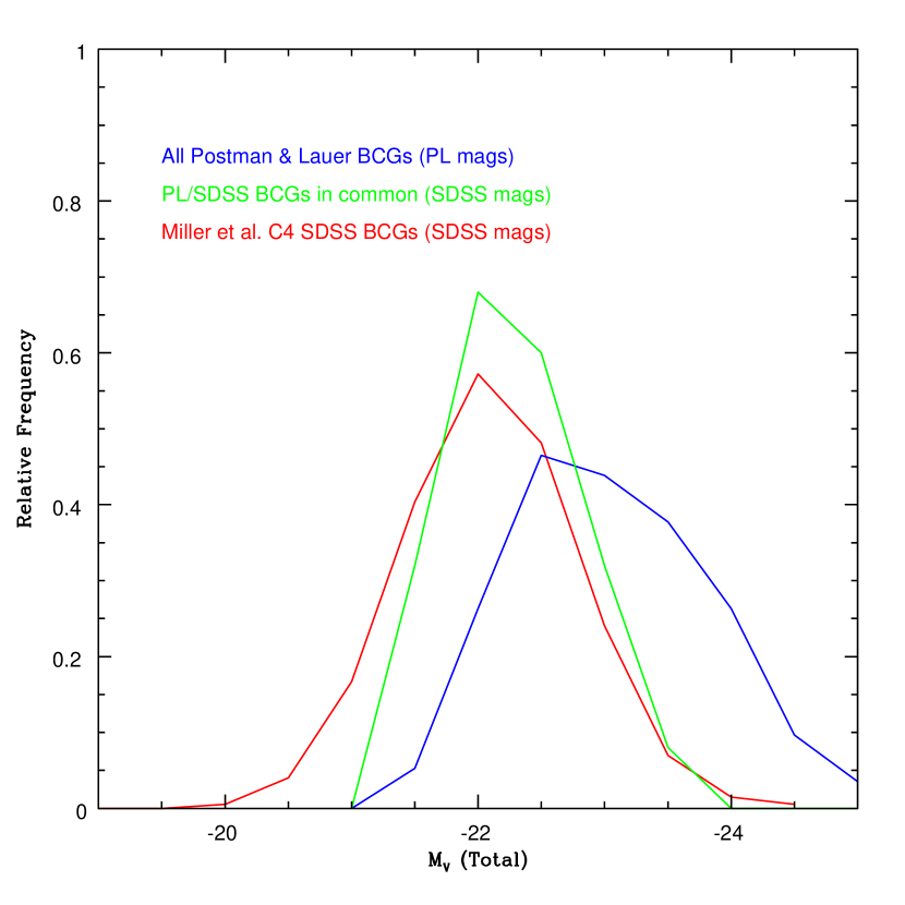
Figure 14: Histograms of estimated total $M_{V}$ are shown for three BCG samples. Magnitudes for the Postman & Lauer (1995) volume-limited BCG sample (blue) are based on $r^{1/4}$ fits to $R_{C}$-band surface photometry. The Miller et al. (2005) BCG sample is based on SDSS model $r$ magnitudes, and has typical luminosities one magnitude smaller than the Postman & Lauer (1995) sample. The histogram of the subset of Postman & Lauer (1995) BCGs observed by SDSS (green) agrees well with the Miller et al. (2005) sample when SDSS $r$ model magnitudes are used instead to estimate total $M_{V},$ yet we argue that these magnitudes are strongly affected by excessive sky subtraction. This concordance implies that the C4 BCGs, are also likely to have had their total luminosities under-estimated.

The large SDSS sky-subtraction errors for bright galaxies may have important implications for the Bernardi et al. (2003) and Blanton et al. (2003) studies, but exactly how is not clear. Both SDSS studies are based on galaxy samples with higher mean redshifts than the Postman & Lauer (1995) sample. Their BCGs should be angularly smaller and thus be less vulnerable to sky subtraction errors. Typical BCGs in the SDSS sample are listed in the Miller et al. (2005) sample of galaxy clusters identified from SDSS galaxy catalogues. Figure 14 shows a histogram of SDSS model $r$ magnitudes (converted to $M_{V}$) for the BCGs identified by Miller et al. (2005) compared to a histogram of all Postman & Lauer (1995) BCGs with $M_{V}$ based on their total $R_{C}$ magnitudes. There is a clear offset between the two samples, with the Postman & Lauer (1995) BCGs appearing to be typically one magnitude brighter than the Miller et al. (2005) BCGs. However, a histogram of SDSS $r$ magnitudes for the 25 Postman & Lauer (1995) BCGs in common with SDSS agrees well with the Miller et al. (2005) BCG histogram, yet these are the magnitudes shown to in be error. We conclude that the total magnitudes of nearby SDSS BCGs are wrong.

Appendix B The Use of Catalogued 2MASS XSC Apparent Luminosities of BCGs

After the first version of this paper was posted on astro-ph, Batcheldor et al. (2006) presented a $M_{\bullet}-L$ relationship for BCGs based on apparent magnitudes extracted from the 2MASS Extended Source Catalogue (XSC) (Jarrett et al., 2000, 2003). The implied NIR luminosity differential between BCGs and other giant elliptical galaxies is greatly reduced from that of the present work. As a result, the plateau in the $L-\sigma$ relationship presented here is greatly reduced in the NIR and the conflict between $M_{\bullet}(\sigma)$ and $M_{\bullet}(L)$ is thus resolved. Batcheldor et al. (2006) further suggest that the relatively higher luminosities inferred from the optical photometry may imply that the envelopes of the BCGs are extremely blue.

We have not conducted a complete comparison of the present photometry with that provided by the 2MASS XSC, but a spot check of a few systems makes it clear that the 2MASS imagery from which the catalogue magnitudes were derived is extremely shallow compared to that of Postman & Lauer (1995), which is the source of the $R$ band optical photometry (transformed to $V$) used in this paper. The most likely explanation for the difference between the present and Batcheldor et al. (2006) results is that the 2MASS images are simply not deep enough to obtain accurate total luminosities of the BCGs, at least as represented by the automatic reductions used to generate the XSC magnitudes.

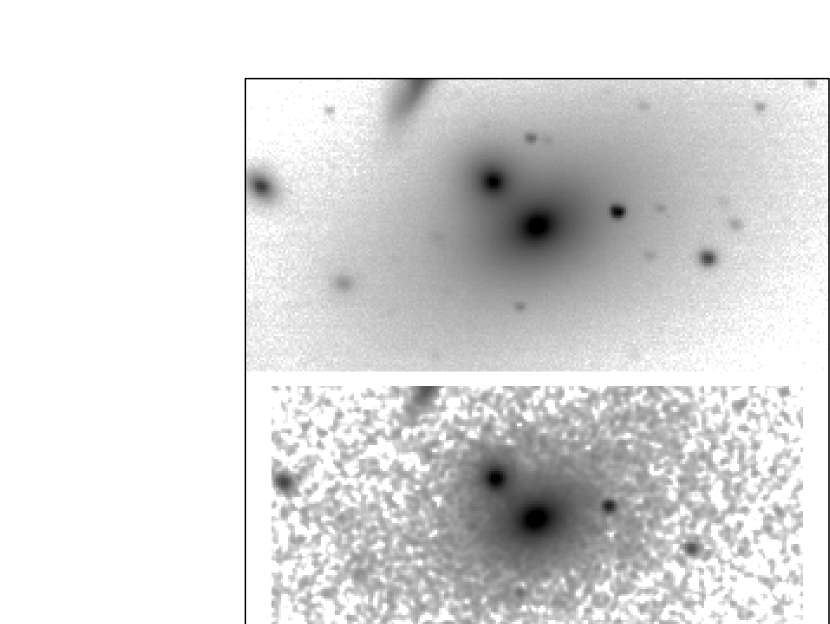
Figure 15: The archived 2MASS $J$ band image of NGC 2832, the BCG in A0779, is compared to a portion of the $R$ band image used by Postman & Lauer (1995) to derive surface photometry profile shown in the next figure. The stretch has been set to be the same for both images. The $R$ band image has been binned to a $0\hbox to1.0pt{}\hbox to0.0pt{${}^{\prime\prime}$\hss}.\hbox to2.0pt{}91$ pixel scale to roughly match the $1\hbox to1.0pt{}\hbox to0.0pt{${}^{\prime\prime}$\hss}.\hbox to2.0pt{}0$ scale of the $J$ band image. The sky level of the 2MASS image is effectively $26\times$ brighter in $J,$ taking the observed $R-J$ color of the galaxy into account. The $J$ band image is clearly considerably shallower than the $R$ band image, and the envelope of the galaxy disappears into the noise at radii where it is still clearly present in the $R$ band.

Figure 15 shows the $J$ band 2MASS image of NGC 2832, the BCG in A0779 compared to the central portion of the $R$ band image obtained by Postman & Lauer (1995). The $J$ sky level is 15.67 magnitudes per square arcsecond versus the $R$ band sky level of 20.90. Accounting for the $R-J=1.68$ color in the center of the galaxy implies that the $J$ band has a sky level effectively $26\times$ brighter. Further, the 2MASS image is a 7.8s exposure obtained with a 1.3m telescope as compared to the 200s $R$ image obtained with a 2.1m telescope (Postman & Lauer, 1995). The $J$ image is thus considerably shallower than the $R$ image as is evident in Figure 15. The galaxy envelope in the $J$ band image disappears into the noise at radii at which it is still clearly present in $R.$ This problem is exacerbated in the $H$ and $K$ bands, which have yet brighter sky levels.

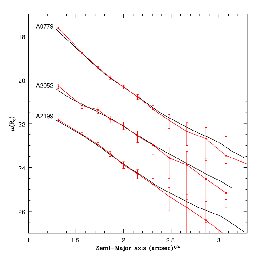
Figure 16: Major axis surface $J$ photometry profiles (red) derived from 2MASS $J$ band archive images are compared to the $R$ profiles derived by Postman & Lauer (1995) (black) for the three BCGs shown in Figure 13. The $\sim 0.4\%$ error in the 2MASS sky levels gives the large error bars. The last $J$ band isophotes fall $\sim 7$ magnitudes below the sky, and thus are less significant than the errors in the sky levels. The $R$ and $J$ profiles agree within the errors, and total luminosities estimated by $r^{1/4}$-law fits to the even the $J$ band profiles are considerably larger than the 2MASS XSC apparent luminosities.

Despite the much brighter $J$ sky level, the $J$ and $R$ band profiles of the A0779 BCG are consistent, as is evident in Figure 16, which compares the $R$ profiles measured by Postman & Lauer (1995) to $J$ profiles derived by us from the 2MASS archive images for the three BCGs shown earlier in Figure 13. The final $J$ band isophote shown for A0779 falls fully $\sim 6.8$ magnitudes below the sky level, but is still in agreement with the $R$ band profile within the large error bars, which represent a 0.004 magnitude error in the 2MASS $J$ sky level.

An $r^{1/4}$ law fitted to the $J$ band profile of A0779 yields $m_{J}=9.04,$ only 0.08 magnitudes fainter than $m_{J}=8.96,$ estimated by subtracting the $R-J=1.68$ color of the central isophotes from $m_{R}$ obtained from the Postman & Lauer (1995) photometry. These values are in poor agreement with the XSC isophotal ($J_{m_{k20fe}}$), and extrapolated ($J_{m_{ext}}$) $m_{J}$ values of 9.78 and 9.67, respectively, however. The isophotal radius, $r_{k20fe},$ is $53\hbox to1.0pt{}\hbox to0.0pt{${}^{\prime\prime}$\hss}.\hbox to2.0pt{}3,$ well interior to the limits of the surface photometry shown in Figure 16. The extrapolated magnitude is based on a Sérsic fit to a surface brightness profile generated by the XSC pipeline. However, even for giant elliptical galaxies the XSC Sérsic index is limited to $n<1.5$ (Jarrett et al. 2003; Jarrett, private communication). The XSC calculation of total magnitudes thus assumes that the galaxies essentially have exponential profiles, rather than the $r^{1/4}$ form standard for giant elliptical galaxies. The XSC pipeline gives $n=1.17$ for A0779, for example, while Graham et al. (1996) find $n>10$ based on the Postman & Lauer (1995) photometry. An exponential cutoff explains both the small difference between the XSC isophotal and total magnitudes, as well as the large deficit of both magnitudes compared to a total magnitude estimated from an $r^{1/4}$ law.

A similar pattern is seen for the two other BCGs shown in Figure 16. For A2052, the BCG has $J_{m_{k20fe}}=10.92,$ corresponding to $r_{k20fe}=38\hbox to1.0pt{}\hbox to0.0pt{${}^{\prime\prime}$\hss}.\hbox to2.0pt{}4,$ and $J_{m_{ext}}=10.60,$ while an $r^{1/4}$ fit to the surface photometry recovered from the 2MASS archive image gives $m_{J}=9.58,$ a full magnitude brighter and only 0.21 magnitudes dimmer than the $m_{J}=9.36$ inferred from the $R$ band imagery with $R-J=1.79.$ For A2199, the BCG (NGC 6166) has $J_{m_{k20fe}}=10.51,$ corresponding to $r_{k20fe}=50\hbox to1.0pt{}\hbox to0.0pt{${}^{\prime\prime}$\hss}.\hbox to2.0pt{}0,$ and $J_{m_{ext}}=10.41,$ generated from a Sérsic fit with $n=1.18$ (Jarrett, private communication); Graham et al. (1996) find $n=6.9.$ An $r^{1/4}$ fit to the surface photometry recovered from the 2MASS archive image gives $m_{J}=9.66,$ 0.75 magnitudes brighter, but 0.41 magnitudes dimmer than $m_{J}=9.20$ inferred from the $R$ band imagery with $R-J=1.82.$

To summarize, our fits to the 2MASS $J$ images for the three BCGs shown give $m_{J}$ values markedly brighter than the XSC apparent magnitudes, but that are much more consistent with the $R$ photometry of Postman & Lauer (1995). As a check, we found that the aperture photometry in Postman & Lauer (1995) interpolated to $r_{k20fe}$ was in excellent agreement with the $J_{m_{k20fe}}$ values, assuming the $R-J$ values derived by comparing the inner portions of the surface photometry profiles; however, $r_{k20fe}$ is well interior to the limits of the optical photometry, thus the XSC isophotal magnitudes cannot be regarded as a total apparent magnitudes. The nearly exponential profile form used by the XSC pipeline explains why $J_{m_{ext}}$ is only modestly brighter than $J_{m_{k20fe}}$ for the three galaxies shown, but is much dimmer than our fits, which assume Sérsic $n=4,$ the standard value for giant elliptical galaxies.

This analysis thus leads us to conclude that the extremely blue BCG envelopes and the relatively modest NIR BCG luminosities advanced by Batcheldor et al. (2006) are artifacts. We do note that the $J$ surface photometry does fall below the $R$ photometry at large radii in all three BCGs, but this occurs for $J$ isophotes well within the noise and well below the even the errors in the sky levels. Any color gradients implied by the profiles presented in Figure 16 are not significant, and in any case are considerably smaller than would be implied by direct comparison of the XSC apparent magnitudes to the parameters given in this paper.

Appendix C The Selection of $r_{\gamma}$ over $r_{b}$ as the Core Scale

The break-radius parameter in the Nuker-law has been used directly as the indicator of physical core scale in earlier work by our group. Faber et al. (1997) showed that $r_{b}$ is correlated with $M_{V}$ for core galaxies. The scatter about the $r_{b}-M_{V}$ relationship is large, however. With the present much larger sample of galaxies, we were able to conduct extensive searches for other parameters that might reduce the scatter, with the goal of better understanding how core structure varies with galaxy properties.

Several plots and parameter fits were conducted to search for correlations between residuals of the $r_{b}-L$ and $r_{b}-\sigma$ relationships with the Nuker profile shape parameters $\alpha,~{}\beta,$ and $\gamma.$ We also tried local values of $\gamma,$ $\gamma^{\prime},$ measured at constant fraction of $r_{b}$ interior to $r_{b}$ ($\gamma^{\prime}(fr_{b})$ with $f<1$). A correlation emerged between the Nuker-law outer profile slope $\beta$ and the residuals in the $r_{b}-L$ relationship, as is shown in Figure 17. Larger than average cores correspond to galaxies with large $\beta$ and vice versa. While one might be tempted to use this relationship to yield some sort of “$\beta$-corrected” break radii, the form of the correlation suggests a simpler, more useful approach. In the Nuker law, $r_{b}$ marks the maximum curvature of the profile in logarithmic coordinates, but also the location where the profile slope reaches the average of $\gamma$ and $\beta.$ Since the range of $\gamma$ for core galaxies is greatly restricted compared to that of $\beta,$ this effectively means that $r_{b}$ will fall at steeper portions of the profile for steeper $\beta.$ This suggests that some sort of “cusp radius,” $r_{\gamma},$ a radius at which the profile reaches a nominal slope value, $\gamma^{\prime},$ would provide a better description of the core scale than $r_{b}.$ The exact definition of $r_{\gamma}$ we use is given in equation (8). Carollo et al. (1997) had already suggested use of $r_{\gamma}$ with $\gamma^{\prime}=1/2,$ the choice that we adopt here.

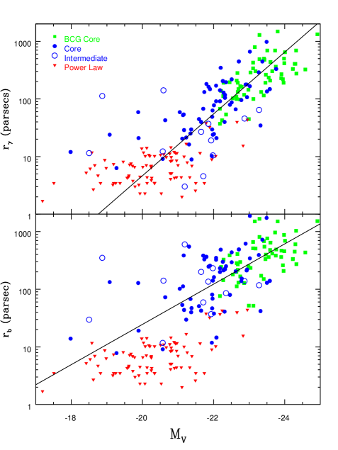
Figure 18: The $r_{\gamma}-L$ and $r_{b}-L$ relationships for core galaxies are compared. The lines are the mean relationships for $M_{V}<-21.$ The $r_{\gamma}-L$ relationship has smaller scatter for core galaxies with $M_{V}<-21.$ Power-law galaxies are plotted the same in both panels, with upper limits on $r_{\gamma}$ to be the same as upper limits on $r_{b}.$

Figure 18 compares the $r_{\gamma}-L$ relationship for $\gamma^{\prime}=1/2$ (shown earlier in Figure 5) and the more traditional $r_{b}-L$ relationship. A symmetrical fit to the latter yields

$$\log(r_{b})=(-0.71\pm 0.04)\left(M_{V}+21.64\right)/2.5+(2.05\pm 0.02),$$ (C1)

which can be compared to the $r_{\gamma}-L$ relation given in equation (10). For most galaxies $\beta>1,$ so in general, $r_{\gamma}<r_{b};$ on average $r_{\gamma}\sim 0.8r_{b}$ for $\gamma^{\prime}=1/2.$ We measured the rms scatter in the $r_{\gamma}-L$ relationship for core galaxies with $M_{V}<-21$ as a function of $\gamma^{\prime}$ over the range $0.4<\gamma^{\prime}<0.7.$ A broad minimum in the scatter of 0.31 in $\log r_{\gamma}$ occurs at $\gamma^{\prime}\sim 1/2.$ This is significantly smaller than the 0.38 scatter in $\log r_{b}$ for the $r_{b}-L$ relationship. The reduced scatter in the $r_{\gamma}-L$ relationship as compared to the $r_{b}-L$ relationship is clearly evident in Figure 18. We have thus chosen to use $r_{\gamma}$ over $r_{b}$ as the core scale.

Evaluation of $r_{\gamma}$ at $\gamma^{\prime}=1/2$ also leads to a clean separation of core and power-law galaxies. Since power-law galaxies have $\gamma^{\prime}>0.5$ at the HST resolution limit, they are naturally excluded from the analysis. The upper limits for $r_{\gamma}$ for power-law galaxies however have the same physical values as their $r_{b}$ limits; since $r_{\gamma}<r_{b}$ for core galaxies, this may create a false impression that the upper limits of $r_{\gamma}$ for power-law galaxies are more in line with the typical $r_{\gamma}$ values of core galaxies.

The issue of whether or not intermediate galaxies can be included within the class of core galaxies, or should be treated separately, unfortunately depends on which relationship is being considered. As is evident in Figure 18, the intermediate galaxies with $M_{V}\leq-21$ appear to be evenly distributed about the the mean $r_{b}-L$ relationship; their mean residual about the relationship is $-0.06\pm 0.15$ in $\log(r_{b}).$ In contrast, the same galaxies fall preferentially to the compact side of the $r_{\gamma}-L$ relationship, now having a mean $\log(r_{\gamma})$ residual of $-0.60\pm 0.11;$ given this systematic offset, we conclude that the intermediate galaxies should be treated separately from the core galaxies.

Table 1: Galaxy Parameters

			$\sigma$		$r_{\gamma}$	$\mu_{\gamma}$
Galaxy	Morph	$M_{V}$	(km/s)	P	$\log({\rm pc})$	(V-Band)	Alt-ID
NGC 0404	S$0-$	$-17.19$	38	$\backslash$	0.23	14.62
NGC 0474	S0	$-20.12$	164	$\backslash$	1.15	15.20
NGC 0507	S0	$-23.02$	311	$\cap$	2.22	16.62
NGC 0524	S0+	$-21.85$	253	$\wedge$	1.57	15.24
NGC 0545	BCG	$-22.98$	242	$\cap$	2.16	16.52	A0194-M1
NGC 0584	E	$-21.38$	207	$\cap$	0.95	14.06
NGC 0596	E	$-20.90$	152	$\backslash$	0.63	13.99
NGC 0720	E	$-22.20$	242	$\cap$	2.54	17.22
NGC 0741	E	$-23.27$	291	$\cap$	2.46	17.48
NGC 0821	E	$-21.71$	200	$\wedge$	0.66	13.75
NGC 0910	BCG	$-22.79$	257	$\cap$	2.21	16.96	A0347-M1
NGC 1016	E	$-22.90$	294	$\cap$	2.25	17.01
NGC 1023	S$0-$	$-20.53$	204	$\backslash$	0.36	12.90
NGC 1052	E	$-21.17$	208	$\cap$	1.46	14.35
NGC 1172	E	$-20.13$	112	$\backslash$	0.64	14.09
NGC 1316	E	$-23.32$	228	$\cap$	1.54	14.30
NGC 1331	E	$-18.58$	58	$\backslash$	1.07	17.07
NGC 1351	S$0-$	$-20.08$	137	$\backslash$	1.01	14.21
NGC 1374	E	$-20.57$	185	$\cap$	0.96	14.57
NGC 1399	E	$-22.07$	342	$\cap$	2.23	16.76
NGC 1400	S$0-$	$-21.37$	256	$\cap$	1.47	15.25
NGC 1426	E	$-20.78$	153	$\backslash$	0.71	14.28
NGC 1427	E	$-20.79$	162	$\backslash$	0.61	14.11
NGC 1439	E	$-20.82$	154	$\backslash$	0.71	13.85
NGC 1500	BCG	$-22.75$	263	$\cap$	1.99	16.34	A3193-M1
NGC 1553	S0	$-22.06$	177	$\backslash$	1.01	13.54
NGC 1600	E	$-23.02$	337	$\cap$	2.82	18.17
NGC 1700	E	$-21.95$	235	$\cap$	1.01	13.50
NGC 2300	S0	$-21.74$	261	$\cap$	2.12	16.82
NGC 2434	E	$-21.33$	188	$\backslash$	0.64	14.60
NGC 2549	S0	$-19.17$	143	$\backslash$	0.51	13.98
NGC 2592	E	$-20.01$	265	$\backslash$	0.82	13.76
NGC 2634	E	$-20.83$	181	$\backslash$	0.93	14.57
NGC 2636	E	$-19.19$	69	$\backslash$	0.87	15.22
NGC 2685	S0+	$-19.72$	94	$\backslash$	0.84	14.16
NGC 2699	E	$-20.25$	141	$\backslash$	0.84	14.14
NGC 2778	E	$-18.75$	162	$\backslash$	0.67	13.97
NGC 2832	BCG	$-23.76$	335	$\cap$	2.52	17.11	A0779-M1
NGC 2841	Sb	$-20.57$	206	$\wedge$	1.09	14.54
NGC 2872	E	$-21.62$	285	$\backslash$	1.06	13.65
NGC 2902	S0	$-20.59$	$\ldots$	$\wedge$	2.15	16.95
NGC 2907	Sa	$-21.23$	$\ldots$	$\backslash$	1.22	13.47
NGC 2950	S0	$-19.73$	182	$\backslash$	0.58	12.99
NGC 2974	E	$-21.09$	227	$\backslash$	0.64	13.77
NGC 2986	E	$-22.32$	262	$\cap$	2.07	16.24
NGC 3056	S0+	$-18.98$	$\ldots$	$\backslash$	0.80	14.10
NGC 3065	S0	$-19.64$	160	$\backslash$	0.86	13.93
NGC 3078	E	$-21.95$	250	$\backslash$	0.95	13.23
NGC 3115	S$0-$	$-21.11$	252	$\backslash$	0.30	12.65
NGC 3193	E	$-21.98$	194	$\cap$	1.38	14.70
NGC 3266	S0	$-20.11$	$\ldots$	$\backslash$	0.85	14.95
NGC 3348	E	$-22.18$	238	$\cap$	1.96	16.05
NGC 3377	E	$-20.07$	139	$\backslash$	0.36	12.24
NGC 3379	E	$-21.14$	207	$\cap$	1.72	15.59
NGC 3384	S$0-$	$-19.93$	148	$\backslash$	0.36	13.03
NGC 3414	S0	$-20.25$	237	$\backslash$	0.81	13.56
NGC 3551	BCG	$-23.55$	268	$\cap$	2.37	17.35	A1177-M1
NGC 3585	E	$-21.93$	207	$\wedge$	1.28	14.29
NGC 3595	E	$-20.96$	$\ldots$	$\backslash$	0.93	14.67
NGC 3599	S0	$-19.93$	85	$\backslash$	0.65	14.64
NGC 3605	E	$-19.61$	92	$\backslash$	0.65	14.96
NGC 3607	S0	$-19.88$	224	$\cap$	1.77	16.26
NGC 3608	E	$-21.12$	193	$\cap$	1.31	15.05
NGC 3610	E	$-20.96$	162	$\backslash$	0.64	12.86
NGC 3613	E	$-21.59$	210	$\cap$	1.65	15.65
NGC 3640	E	$-21.96$	182	$\cap$	1.47	15.39
NGC 3706	S$0-$	$-22.31$	270	$\cap$	1.60	14.16
NGC 3842	BCG	$-23.18$	314	$\cap$	2.48	17.40	A1367-M1
NGC 3900	S0+	$-20.80$	118	$\backslash$	1.16	14.25
NGC 3945	S0+	$-20.25$	174	$\backslash$	0.59	14.19
NGC 4026	S0	$-19.79$	178	$\backslash$	0.48	12.96
NGC 4073	E	$-23.50$	278	$\cap$	2.13	16.55
NGC 4121	E	$-18.53$	86	$\backslash$	0.79	14.55
NGC 4128	S0	$-20.79$	203	$\backslash$	0.92	13.62
NGC 4143	S0	$-19.68$	214	$\backslash$	0.88	13.98
NGC 4150	S0	$-18.66$	85	$\backslash$	0.85	13.87
NGC 4168	E	$-21.80$	184	$\cap$	2.26	17.58
NGC 4239	E	$-18.50$	62	$\wedge$	1.06	16.82
NGC 4261	E	$-22.26$	309	$\cap$	2.31	16.09
NGC 4278	E	$-21.05$	238	$\cap$	1.77	15.82
NGC 4291	E	$-20.64$	285	$\cap$	1.63	15.29
NGC 4365	E	$-22.18$	256	$\cap$	2.15	16.53
NGC 4374	E	$-22.28$	282	$\cap$	2.11	15.67
NGC 4382	S0+	$-21.96$	179	$\cap$	1.69	15.34
NGC 4387	E	$-19.25$	104	$\backslash$	0.54	15.13
NGC 4406	E	$-22.46$	235	$\cap$	1.90	16.03
NGC 4417	S0	$-18.94$	131	$\backslash$	0.94	13.96
NGC 4434	E	$-19.19$	120	$\backslash$	0.54	14.44
NGC 4458	E	$-19.27$	103	$\cap$	0.80	13.57
NGC 4464	E	$-18.82$	127	$\backslash$	0.54	13.92
NGC 4467	E	$-17.51$	68	$\backslash$	0.54	15.07
NGC 4472	E	$-22.93$	291	$\cap$	2.25	16.53
NGC 4473	E	$-21.16$	179	$\cap$	1.73	15.40
NGC 4474	S0	$-18.42$	87	$\backslash$	0.72	14.74
NGC 4478	E	$-19.89$	138	$\cap$	1.32	15.50
NGC 4482	E	$-18.87$	26	$\wedge$	2.05	19.52
NGC 4486	E	$-22.71$	332	$\cap$	2.65	17.25
NGC 4486B	cE	$-17.98$	170	$\cap$	1.08	14.44
NGC 4494	E	$-21.50$	150	$\backslash$	0.54	13.40
NGC 4503	S$0-$	$-19.57$	111	$\backslash$	0.63	14.42
NGC 4551	E	$-19.37$	108	$\backslash$	0.54	14.86
NGC 4552	E	$-21.65$	253	$\cap$	1.60	15.17
NGC 4564	E	$-20.26$	157	$\backslash$	0.63	13.43
NGC 4589	E	$-21.35$	224	$\cap$	1.40	15.41
NGC 4621	E	$-21.74$	225	$\backslash$	0.54	12.43
NGC 4636	E	$-21.86$	203	$\cap$	2.21	16.76
NGC 4648	E	$-20.24$	220	$\backslash$	0.83	13.34
NGC 4649	E	$-22.51$	336	$\cap$	2.34	16.77
NGC 4660	E	$-20.13$	188	$\backslash$	0.54	12.53
NGC 4696	BCG	$-24.33$	254	$\cap$	2.44	17.77	A3526-M1
NGC 4697	E	$-21.49$	174	$\backslash$	0.41	14.13
NGC 4709	E	$-22.32$	242	$\cap$	2.02	16.91
NGC 4742	E	$-19.90$	109	$\backslash$	0.51	12.43
NGC 4874	E	$-23.49$	278	$\cap$	2.99	18.98
NGC 4889	BCG	$-23.73$	401	$\cap$	2.84	17.80	A1656-M1
NGC 5017	E	$-20.67$	184	$\backslash$	0.99	13.30
NGC 5061	E	$-22.01$	186	$\cap$	1.39	14.06
NGC 5077	E	$-22.07$	256	$\cap$	1.96	16.07
NGC 5198	E	$-21.23$	196	$\cap$	1.33	15.19
NGC 5308	S$0-$	$-21.26$	211	$\backslash$	0.90	13.15
NGC 5370	S0	$-20.60$	133	$\backslash$	1.04	15.34
NGC 5419	E	$-23.37$	333	$\cap$	2.65	17.53
NGC 5557	E	$-22.62$	254	$\cap$	1.82	15.58
NGC 5576	E	$-21.31$	183	$\cap$	1.21	14.38
NGC 5796	E	$-21.98$	288	$\wedge$	1.02	14.40
NGC 5812	E	$-21.39$	200	$\backslash$	0.84	14.27
NGC 5813	E	$-22.01$	239	$\cap$	1.89	16.32
NGC 5831	E	$-21.00$	164	$\backslash$	0.85	14.41
NGC 5838	S$0-$	$-20.51$	266	$\backslash$	1.03	13.61
NGC 5845	E	$-19.98$	234	$\backslash$	1.14	13.81
NGC 5898	E	$-21.65$	218	$\wedge$	1.43	15.41
NGC 5903	E	$-21.90$	198	$\cap$	2.17	17.07
NGC 5982	E	$-21.97$	240	$\cap$	1.80	15.62
NGC 6086	BCG	$-23.11$	336	$\cap$	2.53	17.26	A2162-M1
NGC 6166	BCG	$-23.80$	310	$\cap$	3.17	19.32	A2199-M1
NGC 6173	BCG	$-23.59$	278	$\cap$	2.32	16.72	A2197-M1
NGC 6278	S0	$-20.81$	150	$\backslash$	0.99	13.97
NGC 6340	S0	$-19.46$	144	$\backslash$	0.91	14.54
NGC 6849	S0	$-22.78$	216	$\cap$	1.98	16.81
NGC 6876	E	$-23.58$	234	$\cap$	2.17	17.02
NGC 7014	BCG	$-22.18$	263	$\cap$	1.83	15.54
NGC 7052	E	$-22.35$	271	$\cap$	2.29	16.19
NGC 7213	Sa	$-21.71$	182	$\cap$	1.83	15.88
NGC 7332	S0	$-19.62$	124	$\backslash$	0.67	12.78
NGC 7457	S$0-$	$-18.62$	69	$\backslash$	0.43	15.86
NGC 7578B	BCG	$-23.41$	214	$\cap$	2.06	16.19	A2572-M1
NGC 7619	E	$-22.94$	322	$\cap$	2.03	15.90
NGC 7626	E	$-22.87$	276	$\wedge$	1.66	14.98
NGC 7647	BCG	$-23.97$	282	$\cap$	2.28	17.14	A2589-M1
NGC 7727	Sa	$-21.19$	196	$\wedge$	0.48	14.11
NGC 7743	S0+	$-20.18$	84	$\backslash$	1.03	14.07
NGC 7785	E	$-22.08$	245	$\cap$	1.32	15.28
IC 0115	BCG	$-22.67$	$\ldots$	$\cap$	2.45	17.24	A0195-M1
IC 0613	BCG	$-22.27$	262	$\cap$	2.05	16.25	A1016-M1
IC 0664	BCG	$-22.86$	336	$\cap$	2.07	15.81	A1142-M1
IC 0712	BCG	$-23.29$	345	$\cap$	2.69	17.68	A1314-M1
IC 0875	S0	$-20.21$	$\ldots$	$\backslash$	1.01	13.45
IC 1459	E	$-22.51$	306	$\cap$	1.94	15.39
IC 1565	BCG	$-22.99$	303	$\cap$	1.65	16.86	A0076-M1
IC 1633	BCG	$-23.91$	355	$\cap$	2.43	16.66	A2877-M1
IC 1695	BCG	$-23.90$	364	$\cap$	2.36	16.68	A0193-M1
IC 1733	BCG	$-23.43$	301	$\cap$	2.68	17.63	A0260-M1
IC 2738	BCG	$-22.18$	275	$\backslash$	1.57	16.15	A1228-M1
IC 4329	BCG	$-23.95$	275	$\cap$	2.34	16.26	A3574-M1
IC 4931	BCG	$-23.47$	273	$\cap$	2.42	16.86	A3656-M1
IC 5353	BCG	$-22.64$	262	$\cap$	2.04	16.37	A4038-M1
UGC 4551	S0	$-19.78$	167	$\backslash$	0.82	15.00
UGC 4587	S0	$-20.77$	$\ldots$	$\backslash$	1.05	14.79
UGC 6062	S0	$-20.34$	$\ldots$	$\backslash$	1.01	14.66
VCC 1199	E	$-20.34$	$\ldots$	$\backslash$	0.54	15.42
VCC 1440	E	$-20.34$	$\ldots$	$\backslash$	0.54	15.62
VCC 1545	E	$-20.34$	$\ldots$	$\backslash$	0.54	17.49
VCC 1627	E	$-20.34$	$\ldots$	$\backslash$	0.54	15.68
ESO 378-20	S0	$-20.97$	$\ldots$	$\backslash$	1.06	13.11
ESO 443-39	S0	$-20.93$	$\ldots$	$\backslash$	1.06	14.97
ESO 447-30	S0	$-21.17$	$\ldots$	$\backslash$	1.00	13.99
ESO 462-15	E	$-22.83$	305	$\backslash$	1.19	14.75
ESO 507-27	S0	$-20.89$	203	$\backslash$	1.08	14.25
ESO 507-45	S0	$-23.28$	311	$\wedge$	1.81	14.95
MCG 11-14-25A	E	$-19.08$	$\ldots$	$\cap$	1.38	15.77
MCG 08-27-18	S0	$-20.03$	89	$\backslash$	1.07	15.09
A0119-M1	BCG	$-24.01$	294	$\cap$	2.81	18.52
A0168-M1	BCG	$-23.12$	345	$\cap$	2.00	16.90
A0189-M1	BCG	$-21.89$	230	$\backslash$	1.51	17.56
A0261-M1	BCG	$-22.95$	$\ldots$	$\backslash$	1.64	18.22
A0295-M1	BCG	$-23.11$	$\ldots$	$\cap$	2.63	17.81
A0376-M1	BCG	$-23.60$	276	$\cap$	2.64	18.10
A0397-M1	BCG	$-23.42$	289	$\cap$	2.70	17.80
A0419-M1	BCG	$-21.79$	$\ldots$	$\backslash$	1.58	17.08
A0496-M1	BCG	$-24.28$	273	$\cap$	2.61	18.14
A0533-M1	BCG	$-22.68$	$\ldots$	$\cap$	2.28	17.08
A0548-M1	BCG	$-22.75$	220	$\cap$	2.22	17.12
A0634-M1	BCG	$-22.70$	245	$\cap$	2.17	17.16
A0912-M1	BCG	$-22.24$	$\ldots$	$\cap$	1.63	16.36
A0999-M1	BCG	$-22.45$	272	$\cap$	2.29	17.03
A1020-M1	BCG	$-22.65$	345	$\cap$	2.32	16.87
A1631-M1	BCG	$-23.34$	249	$\cap$	2.12	16.49
A1831-M1	BCG	$-23.51$	$\ldots$	$\cap$	2.84	18.58
A1983-M1	BCG	$-22.35$	270	$\wedge$	1.73	15.50
A2040-M1	BCG	$-23.46$	223	$\cap$	2.28	17.41
A2052-M1	BCG	$-23.04$	216	$\cap$	2.46	18.53
A2147-M1	BCG	$-23.16$	278	$\cap$	2.90	19.03
A2247-M1	BCG	$-22.66$	209	$\backslash$	1.60	20.06
A3144-M1	BCG	$-22.28$	$\ldots$	$\cap$	2.28	16.79
A3376-M1	BCG	$-23.29$	300	$\cap$	3.11	18.93
A3395-M1	BCG	$-24.23$	276	$\cap$	2.52	18.09
A3528-M1	BCG	$-24.30$	434	$\cap$	2.61	17.54
A3532-M1	BCG	$-24.58$	$\ldots$	$\cap$	2.51	17.49
A3554-M1	BCG	$-23.99$	$\ldots$	$\cap$	2.62	18.36
A3556-M1	BCG	$-23.65$	$\ldots$	$\cap$	2.48	16.95
A3558-M1	BCG	$-24.92$	275	$\cap$	3.12	19.29
A3562-M1	BCG	$-24.32$	236	$\cap$	2.84	18.87
A3564-M1	BCG	$-22.68$	$\ldots$	$\cap$	2.12	16.63
A3570-M1	BCG	$-22.54$	268	$\cap$	2.01	16.19
A3571-M1	BCG	$-25.30$	325	$\cap$	3.03	19.39
A3677-M1	BCG	$-22.21$	$\ldots$	$\cap$	2.14	16.49
A3716-M1	BCG	$-23.75$	247	$\cap$	2.56	17.99
A3736-M1	BCG	$-23.98$	$\ldots$	$\cap$	2.70	17.93
A3747-M1	BCG	$-22.65$	232	$\cap$	2.00	15.97

Note. — Derivation of the parameters listed are presented in Lauer et al. (2007a). Bulge luminosities are given for S0 and spiral galaxies. Velocity dispersion are provided by the “Hyperleda” database. The profile type, P, is $\backslash=$ power-law, $\wedge=$ intermediate form, and $\cap=$ core. BCG identifications are referred to their hosting Abell clusters; see Postman & Lauer (1995) for details.

Table 2: Core Galaxies with Measured Black Hole Masses

Galaxy	$M_{V}$	$\log(r_{\gamma}/\rm{pc})$	$I_{\gamma}$ (V)	$\log(M_{\bullet}/M_{\odot})$	$M_{\bullet}$ Source
NGC 1399	$-22.07$	2.23	16.76	8.95	1, 2
NGC 3379	$-21.14$	1.72	15.59	8.00	3
NGC 3608	$-21.12$	1.31	15.05	8.28	4
NGC 4261	$-22.26$	2.31	16.09	8.72	5
NGC 4291	$-20.64$	1.63	15.29	8.49	4
NGC 4374	$-22.28$	2.11	15.67	9.00	6, 7
NGC 4473	$-21.16$	1.73	15.40	8.04	4
NGC 4486	$-22.71$	2.65	17.25	9.48	8
NGC 4649	$-22.51$	2.34	16.77	9.30	4
NGC 7052	$-22.35$	2.29	16.19	8.52	9
IC 1459	$-22.51$	1.94	15.39	9.18	10, 11

Note. — Black hole mass references are 1) Houghton et al. (2006), 2) Gebhardt et al. (2007), 3) Gebhardt et al. (2000b), 4) Gebhardt et al. (2003), 5) Ferrarese et al. (1996), 6) Bower et al. (1998), 7) Maciejewski & Binney (2001), 8) Macchetto et al. (1997), 9) van der Marel & van den Bosch (1998), 10) Verdoes Kleijn et al. (2000), and 11) Cappellari et al. (2002). For galaxies with two references, the black hole mass is an average value.

Figure 1: Black hole masses for all black holes with direct mass determinations are plotted as a function of $M_{V}.$ Galaxies are drawn from the Tremaine et al. (2002) sample with augmentations as described in the text. The solid line is the Häring & Rix (2004) relationship (equation (4)) between $M_{\bullet}$ and galaxy mass transformed to luminosity using $M/L_{V}\sim L_{V}^{0.23}$ with zeropoint $M/L_{V}=6$ at $M_{V}=-22.$ A symmetrical least-squares fit to all data points is shown as the dashed line (equation 2), and a fit to just the galaxies with $M_{V}<-19$ is shown as the dotted line (equation 3).

Note that for core galaxies the range in $r_{\gamma}$ at any given $L$ is smaller than it is at a given $\sigma.$

Figure 17: Residuals about the mean $r_{b}-M_{V}$ relationship are plotted for core galaxies as a function of the logarithmic envelope slope $\beta.$ At any given $M_{V},$ excessively large cores (positive residuals) correspond to higher $\beta$ (steeper envelopes) while excessively small cores correspond to small $\beta.$

References

- Adelberger & Steidel (2005) Adelberger, K. L & Steidel, C. C. 2005 ApJ, 630, 50
- Batcheldor et al. (2006) Batcheldor, D., Marconi, A., Merritt, D., & Axon, D. J. 2006, ArXiv Astrophysics e-prints, arXiv:astro-ph/0610264
- Bechtold et al. (2003) Bechtold, J., et al. 2003, ApJ, 588, 119
- Begelman (2006) Begelman, M. C. 2006, ApJ, 643, 1065
- Begelman et al. (1980) Begelman, M. C., Blandford, R. D., & Rees, M. J. 1980, Nature, 287, 307
- Bender et al. (1992) Bender, R., Burstein, D., & Faber, S. M. 1992, ApJ, 399, 462
- Bernardi et al. (2006b) Bernardi, M., Hyde, J. B., Sheth, R. K., Miller, C. J., & Nichol, R. C. 2006b, ArXiv Astrophysics e-prints, arXiv:astro-ph/0607117
- Bernardi et al. (2006c) Bernardi, M., Sheth, R. K., Tundo, E., & Hyde, J. B. 2006c, ArXiv Astrophysics e-prints, arXiv:astro-ph/0609300
- Bernardi et al. (2003) Bernardi, M., et al. 2003, AJ, 125, 1849
- Bernardi et al. (2006a) Bernardi, M., et al. 2006a, AJ, 131, 2018
- Binney & Tabor (1995) Binney, J., & Tabor, G. 1995, MNRAS, 276, 663
- Birnboim & Dekel (2003) Birnboim, Y., & Dekel, A. 2003, MNRAS, 345, 349
- Blanton et al. (2003) Blanton, M. R., et al. 2003, ApJ, 592, 819
- Blumenthal et al. (1984) Blumenthal, G. R., Faber, S. M., Primack, J. R., & Rees, M. J. 1984, Nature, 311, 517
- Bower et al. (2000) Bower, G. A., Wilson, A. S., Heckman, T. M., Magorrian, J., Gebhardt, K., Richstone, D. O., Peterson, B. M., & Green, R. F. 2000, BAAS, 32, 1566
- Bower et al. (1998) Bower, G. A., et al. 1998, ApJ, 492, L111
- Boylan-Kolchin et al. (2006) Boylan-Kolchin, M., Ma, C.-P., & Quataert, E. 2006, MNRAS, 369, 1081
- Cappellari et al. (2002) Cappellari, M., Verolme, E. K., van der Marel, R. P., Kleijn, G. A. V., Illingworth, G. D., Franx, M., Carollo, C. M., & de Zeeuw, P. T. 2002, ApJ, 578, 787
- Carollo et al. (1997) Carollo, C. M., Franx, M., Illingworth, G. D., & Forbes, D. 1997, ApJ, 481, 710
- Churazov et al. (2002) Churazov, E., Sunyaev, R., Forman, W., Böhringer, H. 2002, MNRAS, 332, 729
- de Vaucouleurs et al. (1991) de Vaucouleurs, G., de Vaucouleurs, A., Corwin, H. G., Buta, R. J., Paturel, G., & Fouque, P. 1991, Volume 1-3, XII, 2069 pp. 7 figs.. Springer-Verlag Berlin
- Djorgovski & Davis (1987) Djorgovski, S., & Davis, M. 1987, ApJ, 313, 59
- Dressler (1989) Dressler, A. 1989, IAU Symp. 134: Active Galactic Nuclei, 134, 217
- Dressler et al. (1987) Dressler, A., Lynden-Bell, D., Burstein, D., Davies, R. L., Faber, S. M., Terlevich, R., & Wegner, G. 1987, ApJ, 313, 42
- Ebisuzaki et al. (1991) Ebisuzaki, T., Makino, J., & Okumura, S. K. 1991, Nature, 354, 212
- Faber & Jackson (1976) Faber, S. M., & Jackson, R. E. 1976, ApJ, 204, 668
- Faber et al. (1997) Faber, S. M., Tremaine, S., Ajhar, E. A., Byun, Y., Dressler, A., Gebhardt, K., Grillmair, C., Kormendy, J., Lauer, T. R., & Richstone, D. 1997, AJ, 114, 1771
- Faber et al. (1989) Faber, S. M., Wegner, G., Burstein, D., Davies, R. L., Dressler, A., Lynden-Bell, D., & Terlevich, R. J., 1989, ApJS, 69, 763
- Fabian et al. (2002) Fabian, A. C., Voigt, L. M., & Morris, R. G. 2002, MNRAS, 335, L71
- Ferrarese et al. (1996) Ferrarese, L., Ford, H. C., & Jaffe, W. 1996, ApJ, 470, 444
- Ferrarese & Merritt (2000) Ferrarese, L., & Merritt, D. 2000, ApJ, 539, L9
- Ferrarese et al. (2006) Ferrarese, L., et al. 2006, ApJS, 164, 334
- Fukugita et al. (1995) Fukugita, M., Shimasaku, K., & Ichikawa, T. 1995, PASP, 107, 945
- Gebhardt et al. (2000a) Gebhardt, K., et al. 2000a, ApJ, 539, L13
- Gebhardt et al. (2000b) Gebhardt, K., et al. 2000b, AJ, 119, 1157
- Gebhardt et al. (2003) Gebhardt, K., et al. 2003, ApJ, 583, 92
- Gebhardt et al. (2007) Gebhardt, K., et al. 2007, in preparation
- Gonzalez et al. (2005) Gonzalez, A. H., Zabludoff, A. I., & Zaritsky, D. 2005, ApJ, 618, 195
- Graham et al. (1996) Graham, A., Lauer, T. R., Colless, M., & Postman, M. 1996, ApJ, 465, 534
- Greenhill et al. (1997) Greenhill, L. J., Moran, J. M., & Herrnstein, J. R. 1997, ApJ, 481, L23
- Häring & Rix (2004) Häring, N. & Rix, H. 2004, ApJ, 604, L89
- Harms et al. (1994) Harms, R. J., et al. 1994, ApJ, 435, L35
- Hogg et al. (2004) Hogg, D. W., et al. 2004, ApJ, 601, L29
- Hopkins et al. (2006) Hopkins, P. F., Hernquist, L., Cox, T. J., Di Matteo, T., Robertson, B., & Springel, V. 2006, ApJS, 163, 1
- Houghton et al. (2006) Hougton, R. C. W., Magorrian, J., Sarzi, M., Thatte, N., Davies, R. L., Krajnovic, D. 2006, MNRAS, in press
- Jarrett et al. (2000) Jarrett, T. H., Chester, T., Cutri, R., Schneider, S., Skrutskie, M., & Huchra, J. P. 2000, AJ, 119, 2498
- Jarrett et al. (2003) Jarrett, T. H., Chester, T., Cutri, R., Schneider, S. E., & Huchra, J. P. 2003, AJ, 125, 525
- Kormendy (1985) Kormendy, J. 1985, ApJ, 295, 73
- Kormendy (1993) Kormendy, J. 1993, Coleccion Nuevas Tendencias (The nearest active galaxies), Proceedings of the meeting on The nearest active galaxies, held in Madrid in May 1992, Madrid: Consejo Superior de Investigaciones Cientificas, —c1993, Edited by J. Beckman, L. Colina and H. Netzer, p. 197-218., 197
- Kormendy et al. (2007) Kormendy, J., Fisher, D. B., Cornell, M. E., & Bender, R. 2007, ApJ, submitted
- Kormendy & Richstone (1995) Kormendy, J., & Richstone, D. 1995, ARA&A, 33, 581
- Kormendy et al. (1997) Kormendy, J., et al. 1997, ApJ, 482, L139
- Laine et al. (2002) Laine, S., van der Marel, R. P., Lauer, T. R., Postman, M., O’Dea, C. P., & Owen, F. N. 2003, AJ, 125, 478
- Lauer (1985) Lauer, T. R. 1985, ApJ, 292, 104
- Lauer et al. (1995) Lauer, T. R., et al. 1995, AJ, 110, 2622
- Lauer et al. (2005) Lauer, T. R., et al. 2005, AJ, 129, 2138
- Lauer et al. (2007a) Lauer, T. R., et al. 2007a, ApJ, submitted
- Lauer et al. (2007b) Lauer, T. R., et al. 2007b, in preparation
- Macchetto et al. (1997) Macchetto, F., Marconi, A., Axon, D. J., Capetti, A., Sparks, W., & Crane, P. 1997, ApJ, 489, 579
- Maciejewski & Binney (2001) Maciejewski, W., & Binney, J. 2001, MNRAS, 323, 831
- Magorrian et al. (1998) Magorrian, J., et al. 1998, AJ, 115, 2285
- Marconi et al. (2001) Marconi, A., Capetti, A., Axon, D. J., Koekemoer, A., Macchetto, D., & Schreier, E. J. 2001, ApJ, 549, 915
- Marconi et al. (2004) Marconi, A., Risaliti, G., Gilli, R., Hunt, L. K., Maiolino, R., & Salvati, M. 2004, MNRAS, 351, 169
- McLure et al. (2004) McLure, R. J., Willott, C. J., Jarvis, M. J., Rawlings, S., Hill, G. J., Mitchell, E., Dunlop, J. S., & Wold, M. 2004, MNRAS, 351, 347
- Merritt (2006) Merritt, D. 2006, ApJ, 648, 976
- Miller et al. (2005) Miller, C. J., et al. 2005, AJ, 130, 968
- Milosavljević & Merritt (2001) Milosavljević, M., & Merritt, D. 2001, ApJ, 563, 34
- Naab et al. (2006) Naab, T., Khochfar, S., & Burkert, A. 2006, ApJ, 636, L81
- Nelson et al. (2000) Nelson, C. H., Weistrop, D., Bower, G. A., Green, R. F., & STIS Team 2000, BAAS, 32, 701
- Netzer (2003) Netzer, H. 2003, ApJ, 583, L5
- Novak et al. (2006) Novak, G. S., Faber, S. M., & Dekel, A. 2006, ApJ, 637, 96
- Oegerle & Hoessel (1991) Oegerle, W. R., & Hoessel, J. G. 1991, ApJ, 375, 15
- Patel et al. (2006) Patel, P., Maddox, S., Pearce, F. R., Aragón-Salamanca, A., & Conway, E. 2006, MNRAS, 370, 851
- Postman & Lauer (1995) Postman, M., & Lauer, T. R. 1995, ApJ, 440, 28
- Press et al. (1992) Press, W. H., Teukolsky, S. A., Vetterling, W. T., & Flannery, B. P. 1992, Numerical Recipes (2d ed.; Cambridge: Cambridge Univ. Press)
- Prugniel & Simien (1996) Prugniel, P., & Simien, F. 1996, A&A, 309, 749
- Quillen et al. (2000) Quillen, A. C., Bower, G. A., & Stritzinger, M. 2000, ApJS, 128, 85
- Quinlan (1996) Quinlan, G. D. 1996, New Astronomy, 1, 35
- Quinlan & Hernquist (1997) Quinlan, G. D., & Hernquist, L. 1997, New Astronomy, 2, 533
- Ravindranath et al. (2001) Ravindranath, S., Ho, L. C., Peng, C. Y., Filippenko, A. V., & Sargent, W. L. W. 2001, AJ, 122, 653
- Rest et al. (2001) Rest, A., van den Bosch, F. C., Jaffe, W., Tran, H., Tsvetanov, Z., Ford, H. C., Davies, J., & Schafer, J. 2001, AJ, 121, 2431
- Richards et al. (2005) Richards, G. T., et al. 2005, MNRAS, 360, 839
- Richstone et al. (1998) Richstone, D., et al. 1998, Nature, 395, A14
- Robertson et al. (2006) Robertson, B., Hernquist, L., Cox, T. J., Di Matteo, T., Hopkins, P. F., Martini, P., & Springel, V. 2006, ApJ, 641, 90
- Salpeter (1964) Salpeter, E. E. 1964, ApJ, 140, 796
- Schechter (1976) Schechter, P. 1976, ApJ, 203, 297
- Schlegel et al. (1998) Schlegel, D. J., Finkbeiner, D. P., & Davis, M. 1998, ApJ, 500, 525
- Sérsic (1968) Sérsic, J. L. 1968, Cordoba, Argentina: Observatorio Astronomico, 1968
- Sheth et al. (2003) Sheth, R. K., et al. 2003, ApJ, 594, 225
- Small & Blandford (1992) Small, T. A., & Blandford, R. D. 1992, MNRAS, 259, 725
- Sołtan (1982) Sołtan, A. 1982, MNRAS, 200, 115
- Springel et al. (2005) Springel, V., Di Matteo, T., & Hernquist, L. 2005, MNRAS, 361, 776
- Steidel et al. (2002) Steidel, C. . et al. 2002, ApJ576, 653
- Tadhunter et al. (2003) Tadhunter, C., Marconi, A., Axon, D., Wills, K., Robinson, T. G., & Jackson, N. 2003, MNRAS, 342, 861
- Tonry et al. (2001) Tonry, J. L., Dressler, A., Blakeslee, J. P., Ajhar, E. A., Fletcher, A. B., Luppino, G. A., Metzger, M. R., & Moore, C. B. 2001, ApJ, 546, 681
- Tremaine et al. (2002) Tremaine, S. et al. 2002, ApJ, 574, 740
- Tundo et al. (2006) Tundo, E., Bernardi, M., Hyde, J. B., Sheth, R. K., & Pizzella, A. 2006, ArXiv Astrophysics e-prints, arXiv:astro-ph/0609297
- van der Marel & van den Bosch (1998) van der Marel, R. P., & van den Bosch, F. C. 1998, AJ, 116, 2220
- Verdoes Kleijn et al. (2000) Verdoes Kleijn, G. A., van der Marel, R. P., Carollo, C. M., & de Zeeuw, P. T. 2000, AJ, 120, 1221
- Vestergaard (2004) Vestergaard, M. 2004, ApJ, 601, 676
- Voit & Donahue (2005) Voit, G. M., & Donahue, M. 2005, ApJ, 634, 955
- Wyithe (2006) Wyithe, J. S. B. 2006, MNRAS, 365, 1082
- Wyithe & Loeb (2005) Wyithe, J. S. B., & Loeb, A. 2005, ApJ, 634, 910
- Yu & Lu (2004) Yu, Q., & Lu, Y. 2004, ApJ, 610, 93
- Yu & Tremaine (2002) Yu, Q., & Tremaine, S. 2002, MNRAS, 335, 965
- Zibetti et al. (2005) Zibetti, S., White, S. D. M., Schneider, D. P., & Brinkmann, J. 2005, MNRAS, 358, 949