Phantom Dark Energy Models with Negative Kinetic Term

Abstract

We examine phantom dark energy models derived from a scalar field with a negative kinetic term for which $V(\phi)\rightarrow\infty$ asymptotically. All such models can be divided into three classes, corresponding to an equation of state parameter $w_{\phi}$ with asymptotic behavior $w_{\phi}\rightarrow-1$, $w_{\phi}\rightarrow w_{0}<-1$, and $w_{\phi}\rightarrow-\infty$. We derive the conditions on the potential $V(\phi)$ which lead to each of these three types of behavior. For models with $w_{\phi}\rightarrow-1$, we derive the conditions on $V(\phi)$ which determine whether or not such models produce a future big rip. Observational constraints are derived on two classes of these models: power-law potentials with $V(\phi)=\lambda\phi^{\alpha}$ (with $\alpha$ positive or negative) and exponential potentials of the form $V(\phi)=\beta e^{\lambda\phi^{\alpha}}$. It is shown that these models spend more time in a state with $\Omega_{m}\sim\Omega_{\phi}$ than do corresponding models with a constant value of $w_{\phi}$, thus providing a more satisfactory solution to the coincidence problem.

I Introduction

Observational evidence Knop ; Riess indicates that roughly 70% of the energy density in the universe is in the form of an exotic, negative-pressure component, dubbed dark energy. (See Ref. Copeland for a recent review). If $\rho_{\phi}$ and $p_{\phi}$ are the density and pressure, respectively, of the dark energy, then the dark energy can be characterized by the equation of state parameter $w_{\phi}$, defined by

$$w_{\phi}=p_{\phi}/\rho_{\phi}.$$ (1)

It was first noted by Caldwell Caldwell that observational data do not rule out the possibility that $w_{\phi}<-1$. Such “phantom” dark energy models have several peculiar properties. The density of the dark energy increases with increasing scale factor, and both the scale factor and the phantom energy density can become infinite at a finite $t$, a condition known as the “big rip” Caldwell ; rip ; rip2 . Further, it has been suggested that the finite lifetime for the universe which is exhibited in these models may provide an explanation for the apparent coincidence between the current values of the matter density and the dark energy density doomsday .

The simplest way to achieve a phantom model is to take a scalar field Lagrangian with a negative kinetic term. While such models have certain well-known problems Carroll ; Cline ; Hsu1 ; Hsu2 , they nonetheless provide an interesting set of representative phantom models, and they have been widely studied Guo ; ENO ; NO ; Hao ; Aref ; Peri ; Sami ; Faraoni .

In this paper, we provide a more general analysis of phantom models with negative kinetic terms. In the next section, we reexamine the behavior of such models, and we generalize previous studies to determine the asymptotic behavior of such models and the generic conditions for the existence of a future singularity. In Sec. 3, we derive observational constraints on a subset of these models from the supernova data. In Sec. 4, we examine the solution to the coincidence problem for these models. Our conclusions are summarized in Section 5.

II Phantom Models

II.1 General Results

We limit our discussion to a spatially-flat universe, for which

$$H^{2}=\frac{\rho}{3}$$ (2)

and

$$\dot{\rho}=-3H(\rho+p)\,,$$ (3)

where $H=\dot{a}/a$, $a$ is the scale factor, and we take $\hbar=c=8\pi G=1$ throughout. In equations (2) and (3), $\rho$ and $p$ represent the total energy density and pressure of the matter, radiation, and phantom fields:

$$\rho = \rho_{m}+\rho_{r}+\rho_{\phi},$$ (4)

$$p = p_{r}+p_{\phi}.$$ (5)

In a phantom model with negative kinetic term, the energy density and pressure of the phantom are given by

$$\rho_{\phi}={-(1/2)\dot{\phi}^{2}+V(\phi)},$$ (6)

and

$$p_{\phi}={-(1/2)\dot{\phi}^{2}-V(\phi)},$$ (7)

so that the equation of state parameter is

$$w_{\phi}=\frac{(1/2)\dot{\phi}^{2}+V(\phi)}{(1/2)\dot{\phi}^{2}-V(\phi)}\,,$$ (8)

The evolution equation for this field is

$$\ddot{\phi}+3H\dot{\phi}-V^{\prime}(\phi)=0.$$ (9)

where the prime denotes the derivative with respect to $\phi$. A field evolving according to equation (9) rolls uphill in the potential. If the field gets stuck in a local maximum, we simply have $w_{\phi}=-1$ and no future singularity Carroll ; Hao ; Faraoni . We will confine our attention to models for which $V(\phi)\rightarrow\infty$ asymptotically. (A third possibility is a phantom model for which $V(\phi)$ approaches a constant, e.g., a potential of the form $V(\phi)=V_{0}\phi/(\phi+\phi_{0})$. We will not examine such models here, but they are discussed briefly in Ref. ENO ).

Specific phantom models with $V(\phi)\rightarrow\infty$ have been previously examined in Refs. Guo ; ENO ; NO ; Hao ; Aref ; Peri , while some conditions which produce a future singularity have been examined by Sami and Toporensky Sami and by Faraoni Faraoni . It is these latter studies which we will now generalize.

Sami and Toporensky considered several classes of models, including power-law potentials, $V(\phi)\propto\phi^{\alpha}$ with $\alpha>0$, exponential potentials with $V(\phi)\propto e^{\lambda\phi}$, and potentials steeper than exponential (specifically, $V(\phi)\propto e^{\lambda\phi^{2}}$). They found that the power-law potentials asymptotically produce $w_{\phi}\rightarrow-1$, with a big rip occurring only for the cases with $\alpha>4$. Exponential potentials lead to a big rip with $w_{\phi}$ approaching a constant (see also Refs. ENO ; Hao ), while the $e^{\lambda\phi^{2}}$ potential gives a singularity with $w_{\phi}\rightarrow-\infty$.

Consider first the general relation between the asymptotic behavior of $V(\phi)$ and the asymptotic behavior of $w_{\phi}$. This relation can be derived by writing the equation of motion as Chiba

$$\pm\frac{V^{\prime}}{V}=\sqrt{\frac{-3(1+w_{\phi})}{\Omega_{\phi}}}\left[1+\frac{1}{6}\frac{d\ln(x)}{d\ln(a)}\right],$$ (10)

where $\Omega_{\phi}$ is the density of the phantom field in units of the critical density (note that $\Omega_{\phi}$ evolves with time). In equation (10), $x=\dot{\phi}^{2}/2V$, so that $x$ and $w_{\phi}$ are related via

$$x=-\frac{1+w_{\phi}}{1-w_{\phi}}.$$ (11)

Equation (10) differs slightly from the corresponding equation in Ref. Chiba because we use a different definition of $x$. Equation (10) is the phantom version of the quintessence equation of motion first derived in Ref. Steinhardt ; it differs from the latter equation only in the sign of $1+w$ on the right-hand side.

Now consider the asymptotic evolution of $w_{\phi}$ in the limit where the universe is phantom-dominated. We can distinguish three possible cases, which are determined by the asymptotic behavior of $V^{\prime}/V$ as $V\rightarrow\infty$. Note first that if $V^{\prime}/V$ asymptotically approaches a finite constant, a solution exists for which $w$ approaches a constant; in this case we have $d\ln(x)/d\ln(a)\rightarrow 0$ in equation (10). On the other hand, if $V^{\prime}/V$ becomes asymptotically infinite, we see that there is a solution with $w\rightarrow-\infty$. In this case, $x\rightarrow 1$ (the latter result was noted in the numerical simulations of Ref. Sami ), so that we again have $d\ln(x)/d\ln(a)\rightarrow 0$ in equation (10). Thus, from equation (10), the relation between $V^{\prime}/V$ and $w_{\phi}$ is given by:

Class 1:

$$\frac{V^{\prime}}{V}\rightarrow 0\Leftrightarrow w_{\phi}\rightarrow-1,$$ (12)

Class 2:

$$\frac{V^{\prime}}{V}\rightarrow constant\Leftrightarrow w_{\phi}\rightarrow w_{0}<-1,$$ (13)

Class 3:

$$\frac{V^{\prime}}{V}\rightarrow\pm\infty\Leftrightarrow w_{\phi}\rightarrow-\infty.$$ (14)

These results illuminate the behavior of the specific examples in Refs. Hao ; Sami . For an arbitrary power-law potential, $V\propto\phi^{\alpha}$, we have $V^{\prime}/V=\alpha/\phi$. For positive $\alpha$, $\phi\rightarrow\infty$ and $V^{\prime}/V\rightarrow 0$, so we have $w_{\phi}\rightarrow-1$, as noted in Ref. Sami . On the other hand, if $\alpha<0$, as in the models investigated below, we have $\phi\rightarrow 0$ and $V^{\prime}/V\rightarrow-\infty$, so that $w_{\phi}\rightarrow-\infty$.

The only potential that corresponds exactly to Class 2 is the exponential: $V(\phi)\propto e^{\lambda\phi}$. In this case we see that $w_{\phi}$ approaches a constant; equation (10) gives $w_{\phi}=-1-\lambda^{2}/3$, in agreement with the results of Ref. Hao .

Finally, the potential $V\propto e^{\lambda\phi^{\alpha}}$ gives $V^{\prime}/V=\lambda\alpha\phi^{\alpha-1}$. For $\lambda>0$ and $\alpha>0$, the field rolls in the positive $\phi$ direction, and we see that $V^{\prime}/V\rightarrow 0$ for $\alpha<1$ (so $w_{\phi}\rightarrow-1$), while $V^{\prime}/V\rightarrow\infty$ for $\alpha>1$, so $w_{\phi}\rightarrow-\infty$. For the particular case $\alpha=2$, Sami and Toporensky Sami found $w_{\phi}\rightarrow-\infty$, which agrees with our general result.

Faraoni Faraoni showed that models in which $V(\phi)$ has a vertical asymptote necessarily lead to a singularity in a finite time. All such models fall under our Class 3 (e.g., negative power-law potentials), but there are also models in Class 3 that do not have a vertical asymptote (e.g., $V(\phi)\propto e^{\lambda\phi^{\alpha}}$ with $\lambda>0$ and $\alpha>1$).

All models belonging to Class 2 and Class 3 necessarily lead to a future singularity, but for Class 1, we must distinguish models that produce a big rip from those that do not. In the limit where $w_{\phi}\rightarrow-1$, we have $\dot{\phi}^{2}/2V\rightarrow 0$, and we can neglect the $\ddot{\phi}$ term in equation (9), so that equations (9) and (2) reduce to Sami

$$\dot{\phi}=\frac{V^{\prime}(\phi)}{3H},$$ (15)

and

$$H^{2}=\frac{V(\phi)}{3}.$$ (16)

Combining these two equations gives

$$\dot{\phi}=\frac{V^{\prime}(\phi)}{\sqrt{3V(\phi)}}.$$ (17)

The condition for a big rip is that $V(\phi)$ become infinite in a finite time. From equation (17), this big rip condition is equivalent to the requirement that

$$\int\frac{\sqrt{V(\phi)}}{V^{\prime}(\phi)}d\phi\rightarrow finite$$ (18)

One limit of integration in equation (18) is the value of $\phi$ for which $V\rightarrow\infty$, while the other limit is fixed at an arbitrary constant $\phi_{c}$. Equation (18) distinguishes models with $w_{\phi}\rightarrow-1$ that produce a big rip from those that do not.

Now consider the specific example of the positive power-law potentials. For $V(\phi)=\lambda\phi^{\alpha}$, with $\alpha>0$, the integral in equation (18) becomes

$$\int_{\phi_{c}}^{\infty}\frac{\phi^{\alpha/2}}{\sqrt{\lambda}\alpha\phi^{\alpha-1}}d\phi\propto\phi^{2-\alpha/2}|_{\phi_{c}}^{\infty}$$ (19)

for $\alpha\neq 4$. Clearly, this integral converges (corresponding to a big rip) for $\alpha>4$ and diverges (giving no big rip) for $\alpha<4$, in agreement with the results of Ref. Sami . The case $\alpha=4$ gives an integral that diverges logarithmically, corresponding to no big rip. Again, this agrees with Ref. Sami .

The future singularity that occurs for Class 1 and Class 2 has the property that the scale factor and density both become infinite at a finite time, $t_{s}$. (In the classification scheme of Nojiri, Odintsov, and Tsujikawa NOT , this is a Type I singularity). This need not be the case for Class 3, in which $w_{\phi}\rightarrow-\infty$. As noted in Ref. Sami , the potential $V\propto e^{\lambda\phi^{2}}$ produces a singularity in which the scale factor goes to a constant at finite $t_{s}$, but the density becomes infinite (a Type III singularity in Ref. NOT ). We find that the negative power models investigated in the next section also produce a singularity with finite scale factor and infinite density.

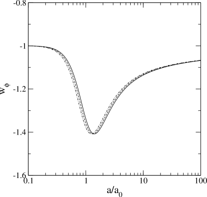
Figure 1: Evolution of the equation of state parameter $w_{\phi}$ as a function of scale factor $a$ ($a_{0}$ is the scale factor today) for $V=\lambda\phi^{2}$ with $\Omega_{m0}=0.25$ (dot-dashed curve), $\Omega_{m0}=0.3$ (dashed curve) and $\Omega_{m0}=0.35$ (solid curve), with $\phi_{0}=1$.

II.2 Specific Cases

II.2.1 Power-Law Potentials

Consider first the case of power-law potentials, for which

$$V(\phi)=\lambda\phi^{\alpha},$$ (20)

and we allow for the exponent $\alpha$ to be either positive or negative. Positive power-law potentials have been previously investigated in Refs. Sami ; Peri ; Guo . Negative power-law potentials have not been previously investigated in general, although Hao and Li Hao showed that such models do not lead to tracker solutions. Note that $\lambda$ in equation (20) is chosen to fix the value of $\Omega_{\phi}$ today, so it is not taken to be a free parameter in these models.

We evolve these models using equation (9).

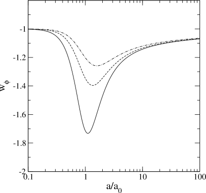
Figure 2: Evolution of the equation of state parameter $w_{\phi}$ as a function of scale factor $a$ ($a_{0}$ is the scale factor today) for $V=\lambda\phi^{2}$ with $\Omega_{m0}=0.3$, and $\phi_{0}=0.5$ (solid curve), $\phi_{0}=1$ (dashed curve), and $\phi_{0}=1.5$ (dot-dashed curve).

We take $\dot{\phi}=0$ initially, but we have verified that the evolution is independent of this initial condition. As long as $\rho_{\phi}\ll\rho_{m}+\rho_{r}$, $\dot{\phi}$ quickly decays to zero. On the other hand, we do find that these models are highly sensitive to the initial value for $\phi$, which we designate as $\phi_{0}$. This contrasts sharply with the behavior of ordinary quintessence models with power-law potentials, for which the evolution can be insensitive to the initial conditions Steinhardt ; LS . The actual value of $\phi_{0}$ is, of course, a model-dependent quantity. (For quintessence models, some estimates of plausible values of $\phi_{0}$, produced by quantum fluctuations during inflation, have been derived by Malquarti and Liddle phi0 ). In this paper, we simply emphasize that many of our results are very sensitive to the assumed value of $\phi_{0}$.

We now present two representative examples, the case $V(\phi)=\lambda\phi^{2}$, which does not lead to a big rip, and the case $V(\phi)=\lambda\phi^{6}$, which does yield a big rip. Fig. 1 shows the evolution of the equation of state parameter $w_{\phi}$ for $V=\lambda\phi^{2}$ with a fixed value of $\phi_{0}$ ($\phi_{0}=1$, in the units defined in Sec. II.A.), and $\Omega_{m0}=0.25,0.30,0.35$ (where $\Omega_{m0}$ is the present-day matter density in units of the critical density). Note that equation (10) implies that for a fixed set of initial conditions, there is a single functional behavior for $w_{\phi}$ as a function of $\Omega_{\phi}$. Hence, we can simply calculate $w_{\phi}$ as a function of $\Omega_{m}$ and define the “present” to be the point at which $\Omega_{m}$ evolves to the given desired value, $\Omega_{m0}$. This implies that the three curves for $w(a)$ differ only in an overall multiplicative constant for $a$; on the log scale in Fig. 1, the three curves are therefore identical and are simply displaced horizontally from each other. Given this simple dependence on $\Omega_{m0}$, and the fairly narrow observational limits on $\Omega_{m0}$, we choose to fix the value of $\Omega_{m0}$ to be $\Omega_{m0}=0.3$ thoughout the rest of this paper.

In Fig. 2, we show the evolution of $w_{\phi}$ for the same power-law potential for three different values of $\phi_{0}$ ($\phi_{0}=0.5,1,1.5$). Here we see a much wider divergence in the evolution of these models.

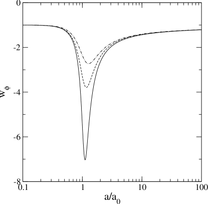
Figure 3: Evolution of the equation of state parameter $w_{\phi}$ as a function of scale factor $a$ ($a_{0}$ is the scale factor today) for $V=\lambda\phi^{6}$ with $\Omega_{m0}=0.3$, and $\phi_{0}=0.5$ (solid curve), $\phi_{0}=1$ (dashed curve), and $\phi_{0}=1.5$ (dot-dashed curve).

Fig. 3 gives the evolution of $w_{\phi}$ for the power-law potential $V=\lambda\phi^{6}$ and three different values for $\phi_{0}$. We note that for both power laws, $w_{\phi}\approx-1$ at early times, but then $w_{\phi}$ decreases sharply as soon as $\rho_{\phi}$ becomes comparable to $\rho_{m}$. Then $w_{\phi}$ asymptotically returns to $-1$ at late times. This behavior is consistent with the results for the single power-law model [$V(\phi)=\lambda\phi^{2}$] investigated in Ref. Sami .

Now consider negative power-law potentials. In Figs. 4 and 5, we show the evolution of $w_{\phi}$ for two negative power-law models: $V=\lambda\phi^{-1}$ and $V=\lambda\phi^{-2}$. As for the positive power-law models, these models begin with $w_{\phi}\approx-1$, but, as noted in the previous section, $w_{\phi}$ generically evolves toward $-\infty$. The change in behavior from $w_{\phi}\approx-1$ to $w_{\phi}\rightarrow-\infty$ is triggered by $\rho_{\phi}$ dominating the expansion. Again, we see that the evolution is quite sensitive to the initial value of $\phi$. For small values of $\phi_{0}$ ($\phi_{0}\lesssim 0.5$), these models yield a singularity at the present, a result not favored by observations.

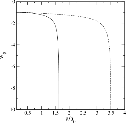
Figure 4: Evolution of the equation of state parameter $w_{\phi}$ as a function of scale factor $a$ ($a_{0}$ is the scale factor today) for $V=\lambda\phi^{-1}$ with $\Omega_{m0}=0.3$ and $\phi_{0}=1$ (solid curve), $\phi=1.5$ (dashed curve).

II.2.2 Exponential Potentials

Now consider a second class of models of the form

$$V(\phi)=\beta\exp\left(\lambda\phi^{\alpha}\right).$$ (21)

For simplicity, we will consider only the case $\lambda>0$. As for the power-law case, it is clear from equation (10) that the functional form of $w_{\phi}(\Omega_{\phi})$ is independent of $\beta$, since $V^{\prime}/V$ is independent of $\beta$, so we choose $\beta$ to give the desired value of $\Omega_{m0}$.

Using our classification scheme of Sec. II.A., we find that

$$\frac{V^{\prime}}{V}=\lambda\alpha\phi^{\alpha-1}$$ (22)

with the field rolling in the positive $\phi$ direction. Hence, the asymptotic behavior of $w_{\phi}$ depends on the value of $\alpha$. For $\alpha=1$, equation (21) reduces to a simple exponential, previously investigated in Refs. ENO ; Hao ; Sami . In this case $w_{\phi}\approx-1$ initially, with $w_{\phi}$ evolving to the value $w_{\phi}=-1-\lambda^{2}/3$ at late times Hao . As noted in the previous section, this is the only scalar field model with negative kinetic term that corresponds exactly to Class 2 ($w_{\phi}=w_{0}\neq-1$ at late times). For $\alpha>1$, we see from equation (22) that $V^{\prime}/V\rightarrow\infty$ asymptotically, so that $w_{\phi}\rightarrow-\infty$ at late times.

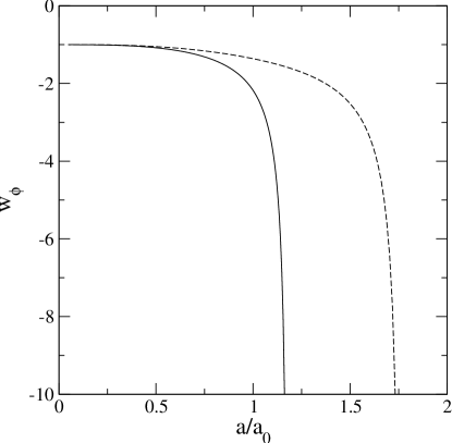
Figure 5: Evolution of the equation of state parameter $w_{\phi}$ as a function of scale factor $a$ ($a_{0}$ is the scale factor today) for $V=\lambda\phi^{-2}$ with $\Omega_{m0}=0.3$ and $\phi_{0}=1$ (solid curve), $\phi=1.5$ (dashed curve).

(The special case of $\lambda=1,\alpha=2$ was investigated in Ref. Sami ). Finally, for $\alpha<1$, we see that $V^{\prime}/V\rightarrow 0$ asymptotically, so that $w_{\phi}\rightarrow-1$ at late times. For these models, the question of whether or not a big rip occurs is determined by equation (18). We see that

$$\int\frac{\sqrt{V(\phi)}}{V^{\prime}(\phi)}d\phi=\int_{\phi_{c}}^{\infty}\frac{1}{\lambda\alpha\sqrt{\beta}}\phi^{1-\alpha}e^{-\lambda\phi^{\alpha}/2}d\phi$$ (23)

For $0<\alpha<1$, this integral always converges, which indicates that for these cases we get a big rip.

The behavior of several representative examples of these models is illustrated in Figs. 6 and 7. For these models, we take $\phi_{0}=1$, although the case $\alpha=1$ (only) is insensitive to the initial conditions. For all of these models, the transition in $w_{\phi}$ is triggered by the onset of dark energy domination, as was the case for the power-law potentials.

III Supernova Constraints on Phantom Models

Supernova Ia observations Knop ; Riess provide the best current constraints on the value of $w_{\phi}$. However, these limits normally assume either a constant $w_{\phi}$, or a value for $w_{\phi}$ that varies linearly with $a$ near the present. The phantom models discussed here clearly display quite different behavior for the evolution of $w_{\phi}$. Hence, it is useful to derive supernova constraints for these models directly.

In this section, we investigate the goodness of fit of various phantom models to the corresponding observed luminosity distance $D_{L}^{obs}$ coming from the SnIa Gold data set Riess .

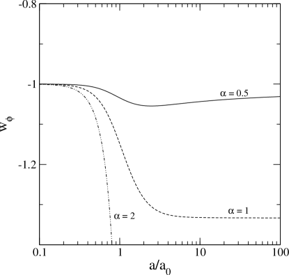
Figure 6: Evolution of the equation of state parameter $w_{\phi}$ as a function of scale factor $a$ ($a_{0}$ is the scale factor today) for the exponential potential $V=\beta e^{\lambda\phi^{\alpha}}$, with $\lambda=1$, $\Omega_{m0}=0.3$, and $\phi_{0}=1$, for the indicated values of $\alpha$.

The observations of supernovae measure essentially the apparent magnitude $m$, which is related to the luminosity distance $d_{L}$ by

$$m(z)={\cal M}+5\log_{10}D_{L}(z)~{},$$ (24)

where

$$D_{L}(z)\equiv{\frac{H_{0}}{c}}d_{L}(z)~{},$$ (25)

is the dimensionless luminosity distance and

$$d_{L}(z)=(1+z)d_{M}(z)~{},$$ (26)

with $d_{M}(z)$ being the comoving distance given by

$$d_{M}(z)=c\int_{0}^{z}{\frac{1}{H(z^{\prime})}}dz^{\prime}~{}.$$ (27)

Also,

$${\cal M}=M+5\log_{10}\left({\frac{c/H_{0}}{1~{}\mbox{Mpc}}}\right)+25~{},$$ (28)

where $M$ is the absolute magnitude.

The data points in these samples are given in terms of the distance modulus

$$\mu_{\rm obs}(z)\equiv m(z)-M(z)~{}=5\log d_{L}+25,$$ (29)

where $d_{L}$ is measured in Mpc. The $\chi^{2}$ is calculated from

$$\chi^{2}=\sum_{i=1}^{n}\left[{{\mu_{\rm obs}(z_{i})-\mu_{\rm th}(z_{i};H_{0},c_{\alpha})}\over{\sigma_{\mu_{\rm obs}}(z_{i})}}\right]^{2}~{},$$ (30)

where the present-day Hubble parameter, $H_{0}$, is a nuisance parameter that is marginalized over, and $c_{\alpha}$ are the model parameters.

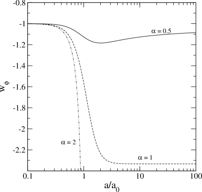
Figure 7: As Fig. 6, for $\lambda=2$.

In what follows, we study $\Delta\chi^{2}$ given by

$$\Delta\chi^{2}=\chi^{2}-\chi^{2}_{lcdm}$$ (31)

where $\chi^{2}_{lcdm}=177.1$ is the value for the $\Lambda$CDM model with $\Omega_{m}=0.3$ and $\Omega_{\Lambda}=0.7$, which we take as our fiducial model, as it provides a good fit to all current cosmological observations. Thus, $\Delta\chi^{2}$ measures how much worse (or better, for $\Delta\chi^{2}<0$) the phantom model fits the data compared to the standard $\Lambda$CDM model.

The value of $\Delta\chi^{2}$ for the potentials $V=\lambda\phi^{\alpha}$ is shown in Fig. 8 as a function of $\alpha$. (In this section, we take $\phi_{0}=1$ throughout). It is clear that large positive or negative values of $\alpha$ are excluded. At the $2\sigma$ level, we have

$$-1.5<\alpha<2.$$ (32)

A comparison of these limits with the evolution graphs for $w_{\phi}$ in Sec. II. B. shows, not surprisingly, that the best agreement with the observations occurs for models which most closely resemble a cosmological constant up to the present. The allowed models with negative power-law potentials generically resemble a cosmological constant at early times, deviating toward large negative values of $w_{\phi}$ and a singularity at late times. In this regard, they resemble some variants of the Chaplygin gas model Sen . Positive power-law models with large $\alpha$, which correspond to more negative values of $w_{\phi}$ at the present, are excluded. In particular, we must have $\alpha>4$ to produce a big rip, and all such models are excluded by observations. Note, however, that we have confined our investigation to the initial state $\phi_{0}=1$; these conclusions will differ for other values of $\phi_{0}$.

The value of $\Delta\chi^{2}$ for the exponential potentials, $V=\beta e^{\lambda\phi^{\alpha}}$ is shown in Fig. 9. The likelihood here is obviously a function of both $\lambda$ and $\alpha$, but it is clear that smaller values of $\alpha$ are favored. Conservative limits are $\alpha<1.5$ for $\lambda=1$ and $\alpha<1$ for $\lambda<2$. Within these limits, models with $\lambda=1$ allow all three classes of behavior for the asymptotic value of $w_{\phi}$, as defined in Sec. II. A. However, with $\lambda>2$, we see that only $\alpha<1$ is allowed, corresponding to $w_{\phi}\rightarrow-1$ asymptotically. As noted, however, these $\alpha<1$ models do produce a big rip at late times.

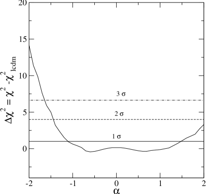
Figure 8: The value of $\Delta\chi^{2}=\chi^{2}-\chi^{2}_{lcdm}$ as a function of $\alpha$ for the power-law potentials $V=\lambda\phi^{\alpha}$, with $\Omega_{m0}=0.3$ and $\phi_{0}=1$. Here $\chi^{2}_{lcdm}$ is the value of $\chi^{2}$ for the $\Lambda$CDM model with $\Omega_{m0}=0.3$ and $\Omega_{\Lambda 0}=0.7$. Horizontal lines give the $1\sigma$, $2\sigma$, and $3\sigma$ limits.

IV Coincidence Analysis

This section is an extension of the coincidence analysis of Ref. doomsday to the models outlined in the previous section. Observational evidence suggests that the matter density and the dark energy density have similar values today. However, for a cosmological constant (for instance), we have $\rho_{\Lambda}$ constant, $\rho_{m}\propto a^{-3}$, so there is only a very small epoch in time when these two densities are within an order of magnitude of each other; this constitutes the “coincidence problem.”

Scherrer doomsday argued that phantom models provide a natural explanation of this result, since the big rip in such a universe is itself triggered by the onset of phantom domination. Hence, the universe spends an appreciable fraction of its total lifetime in a “coincidental” state, with $\rho_{\phi}\approx\rho_{m}$. (Extensions and elaborations of this argument can be found in Refs. Avelino ; Cai ; Yang ).

As in Ref. doomsday we define the parameter $r$ to be the ratio of scalar field energy density to nonrelativistic matter density:

$$r\equiv\frac{\rho_{\phi}}{\rho_{m}}.$$ (33)

For a universe with a future singularity, we then calculate the fraction of the total (finite) lifetime of the universe that is spent in a state for which the two energy densities are within a factor of $r_{0}$ from each other: $1/r_{0}<r<r_{0}$.

This fraction $f$ can be derived by first calculating the total lifetime of the universe, given by

$$t_{U}=\int_{0}^{\infty}\frac{da}{aH(a)}\,.$$ (34)

and comparing it to the time that the universe spends in expanding from an initial scale factor, $a_{1}$, to a final scale factor $a_{2}$:

$$t_{12}=t_{2}-t_{1}=\int_{a_{1}}^{a_{2}}\frac{da}{aH(a)}\,,$$ (35)

where we choose the scale factors to correspond to energy density ratios of $r_{1}=1/r_{0}$ for $a_{1}$ and $r_{2}=r_{0}$ for $a_{2}$. The coincidence fraction $f$ is then given by

$$f=t_{12}/t_{U}\,,$$ (36)

which tells us the fraction of time that the energy densities are within a factor of $r_{0}$ from each other.

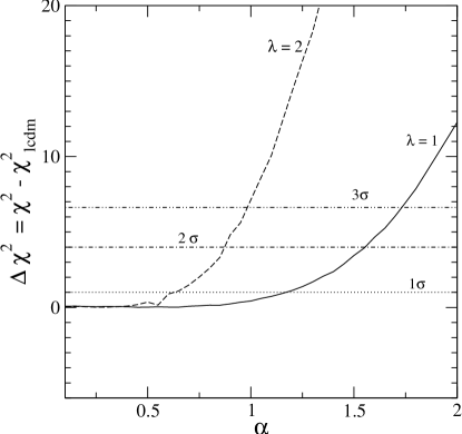
Figure 9: As Fig. 8, for the exponential potentials $V=\beta e^{\lambda\phi^{\alpha}}$, with $\lambda=1$ and $\lambda=2$.

For phantom models with constant $w_{\phi}$, this coincidence fraction can be expressed as doomsday

$$f=\frac{\Gamma(1/2)}{\Gamma(-\frac{1}{2w})\Gamma(\frac{1}{2}+\frac{1}{2w})}\int_{1/r_{0}}^{r_{0}}\frac{r^{-(2w+1)/2w}}{\sqrt{1+r}}dr.$$ (37)

A larger value of $f$ corresponds to a universe in which it is more natural to observe $\Omega_{\phi}\sim\Omega_{m}$ today, ameliorating the coincidence problem.

Note that the choice of $r_{0}$ is somewhat arbitrary; in this paper we choose $r_{0}=10$, corresponding to $\rho_{\phi}$ and $\rho_{m}$ lying within an order of magnitude of each other.

Figure 10: Solid curve gives the fraction of time $f$ that the universe spends in a state with $0.1<\rho_{\phi}/\rho_{m}<10$, for phantom models with $V(\phi)=\lambda\phi^{\alpha}$; $f$ is given as a function of $\alpha$. Dashed curve gives $f$ for models with constant $w_{\phi}$ having the same value of $w_{\phi}$ at the present as the corresponding power-law model.

Since our goal is to compare scalar field phantom models with constant-$w_{\phi}$ phantom models, the actual value of $r_{0}$ is not crucial. Further, we note that the value of $f$, like the evolution of the scalar field, depends on the initial value for $\phi_{0}$. For definiteness, we consider only $\phi_{0}=1$ in what follows, but these results are easily extended to other values of $\phi_{0}$.

In Fig. 10, we show the coincidence fraction $f$ for the power-law models $V(\phi)\propto\phi^{\alpha}$ as a function of $\alpha$, for the range of values of $\alpha$ that is not ruled out at the $2\sigma$ level (cf. Fig. 8). No positive values for $\alpha$ are displayed, since only the region $\alpha<2$ is consistent with the supernova data, while a future singularity can occur only for $\alpha>4$, and only models with a future singularity are relevant in this coincidence analysis. Within the allowed range for $\alpha$, the value of $f$ can be quite large, roughly 0.7 for the most negative allowed values of $\alpha$. This means that the universe spends 70% of its lifetime in a “coincidental” state, i.e., one in which the matter and dark energy densities lie within an order of magnitude of each other.

Further, we note that these scalar-field-based phantom models provide a more satisfactory solution to the coincidence problem than the corresponding models with constant $w_{\phi}$ (such as those discussed in Ref. doomsday ) in the sense that the former models yield a significantly larger value for $f$ for a given current value of $w_{\phi}$. The physical explanation for this lies in the way in which $w_{\phi}$ evolves in the models with negative power law potentials. In these models, just as in the constant-$w_{\phi}$ models, the onset of the singularity is triggered by the dominance of the dark energy component. However, in the scalar field models, the beginning of phantom dominance also triggers a rapid decrease in $w_{\phi}$, producing an even more rapid evolution toward the singularity.

In Fig. 11, we show the coincidence fraction $f$ for the exponential models $V(\phi)=\beta e^{\lambda\phi^{\alpha}}$ for $\lambda=1$. Note that this figure encompasses all three classes of behavior discussed in Sec. II.A. For $\alpha<1$, we have $w_{\phi}\rightarrow-1$ (with a big rip), for $\alpha=1$, we have $w_{\phi}\rightarrow-4/3$ and for $\alpha>1$ we have $w_{\phi}\rightarrow-\infty$.

Figure 11: As Fig. 10, for exponential potential $V(\phi)=\beta e^{\lambda\phi^{\alpha}}$, with $\lambda=1$.

Again, we see that over most of the allowed range for $\alpha$, the scalar field models yield a larger value for $f$ than do the corresponding constant-$w_{\phi}$ models with the same present-day value for $w_{\phi}$.

V Conclusions

Our results provide a comprehensive classification of phantom models with negative kinetic term for which $V(\phi)\rightarrow\infty$ asymptotically. All such models lead to either $w_{\phi}\rightarrow-1$, $w_{\phi}\rightarrow w_{0}<-1$, or $w_{\phi}\rightarrow-\infty$, depending on the asymptotic form of the potential. The first set of these models need not lead inevitably to a big rip singularity; we have derived the conditions on $V(\phi)$ which determine when a big rip occurs. Our results agree with all of the specific cases that have been previously investigated elsewhere.

Power-law potentials of the form $V=\lambda\phi^{\alpha}$ lead to $w_{\phi}\rightarrow-1$ for positive power laws and $w_{\phi}\rightarrow-\infty$ for negative power laws. However, the supernova observations provide both upper and lower bounds on $\alpha$. For the set of initial conditions on $\phi$ considered here, the only models which are both consistent with the observations and lead to a future singularity are the negative power-law potentials.

Generalized exponentials of the form $V=\beta e^{\lambda\phi^{\alpha}}$ can lead to all three sorts of behaviors indicated above. We have $w_{\phi}\rightarrow-1$ for $\alpha<1$, $w_{\phi}\rightarrow w_{0}$ for $\alpha=1$ and $w_{\phi}\rightarrow-\infty$ for $\alpha>1$. The supernova observations favor smaller values of $\alpha$; for the initial conditions examined here, we find that $\alpha<1.5$ for $\lambda=1$ and $\alpha<1$ for $\lambda=2$.

These observational limits must be treated with some caution, as they are highly sensitive to the assumed initial conditions. For the specific potentials considered here (power laws and generalized exponentials) we find that the evolution of the scalar field is very sensitive to the initial value of $\phi$ (but not $\dot{\phi}$), in contrast to the “tracker” quintessence models. Nonetheless, these limits do provide a clue to the general forms of the most observationally-favored models: not surprisingly, they are the models which most closely resemble a cosmological constant.

Finally, we have considered the solution of the coincidence problem in the context of these phantom models. This argument relies on the idea that a universe with a future singularity has a finite lifetime, so it is possible to calculate the fraction of that lifetime, $f$, for which the densities of the matter and dark energy lie within an order of magnitude of each other. Over the observationally-allowed parameter range, we find that both the power-law potentials and the exponential potentials yield a larger value for $f$ than do the corresponding constant-$w_{\phi}$ models (examined in Ref. doomsday ) with the same present-day value for $w_{\phi}$. Thus, these phantom models with time-varying $w_{\phi}$ provide a better resolution of the coincidence problem than do constant-$w_{\phi}$ phantom models. This is particularly true for models in which $w_{\phi}$ decreases with time, as such models lead to a faster evolution toward the singularity.

It is clear that phantom models arising from scalar fields with negative kinetic terms produce a rich set of behaviors. The class of such models that is consistent with current cosmological observations yields a variety of different possible future fates for the universe.

- (1) R.A. Knop, et al., Ap.J. 598, 102 (2003).
- (2) A.G. Riess, et al., Ap.J. 607, 665 (2004).
- (3) E.J. Copeland, M. Sami, and S. Tsujikawa, hep-th/0603057.
- (4) R.R. Caldwell, Phys. Lett. B 545, 23 (2002).
- (5) R.R. Caldwell, M. Kamionkowski, and N.N. Weinberg, Phys. Rev. Lett. 91, 071301 (2003).
- (6) S. Nesseris and L. Perivolaropoulos, Phys. Rev. D70, 123529 (2004).
- (7) R.J. Scherrer, Phys. Rev. D71, 063519 (2005).
- (8) S.M. Carroll, M. Hoffman, and M. Trodden, Phys. Rev. D68, 023509 (2003).
- (9) J.M. Cline, S. Jeon, and G.D. Moore, Phys. Rev. D70, 043543 (2004).
- (10) R.V. Buniy and S.D.H. Hsu, Phys. Lett. B 632, 543 (2006).
- (11) R.V. Buniy, S.D.H. Hsu, and B.M. Murray, hep-th/0606091.
- (12) Z.-K. Guo, Y.-S. Piao, and Y.-Z. Zhang, Phys. Lett. B 594, 247 (2004).
- (13) E. Elizalde, S. Nojiri, and S.D Odintsov, Phys. Rev. D70, 043539 (2004).
- (14) S. Nojiri and S.D. Odintsov, Phys. Rev. D70, 103522 (2004).
- (15) J.-G. Hao and X.-Z. Li, Phys. Rev. D70, 043529 (2004).
- (16) I. Ya. Aref’eva, A.S. Koshelev, and S. Yu. Vernov, astro-ph/0412619.
- (17) L. Perivolaropoulos, Phys. Rev. D71, 063503 (2005).
- (18) M. Sami, A. Toporensky, Mod. Phys. Lett. A 19, 1509 (2004).
- (19) V. Faraoni, Class. Quant. Grav. 22, 3235 (2005).
- (20) T. Chiba, Phys. Rev. D73, 063501 (2006).
- (21) P.J. Steinhardt, L. Wang, and I. Zlatev, Phys. Rev. D59, 123504 (1999).
- (22) S. Nojiri, S.D. Odintsov, and S. Tsujikawa, Phys. Rev. D71, 063004 (2005).
- (23) A.R. Liddle and R.J. Scherrer, Phys. Rev. D 59, 023509 (1999).
- (24) M. Malquarti and A.R. Liddle, Phys. Rev. D66, 023524 (2002).
- (25) A.A. Sen and R.J. Scherrer, Phys. Rev. D72, 063511 (2005).
- (26) P.P. Avelino, Phys. Lett. B 611, 15 (2005).
- (27) R.-G. Cai and A. Wang, JCAP 0503, 002 (2005).
- (28) G. Yang and A. Wang, Gen. Rel. Grav. 37, 2201 (2005).