The Einstein ring 0047-2808 Revisited: A Bayesian Inversion

Abstract

In a previous paper, we outlined a new Bayesian method for inferring the properties of extended gravitational lenses, given data in the form of resolved images. This method holds the most promise for optimally extracting information from the observed image, whilst providing reliable uncertainties in all parameters. Here, we apply the method to the well studied optical Einstein ring 0047-2808. Our results are in broad agreement with previous studies, showing that the density profile of the lensing galaxy is aligned within a few degrees of the light profile, and suggesting that the source galaxy (at redshift 3.6) is a binary system, although its size is only of order 1-2 kpc. We also find that the mass of the elliptical lensing galaxy enclosed by the image is (2.91$\pm$0.01)$\times$10¹¹ M_☉. Our method is able to achieve improved resolution for the source reconstructions, although we also find that some of the uncertainties are greater than has been found in previous analyses, due to the inclusion of extra pixels and a more general lens model.

1. Introduction

Gravitational lenses have long held the promise of being natural telescopes, probing structural scales smaller than the resolution of current technologies while simultaneously revealing the distribution of matter within the lensing galaxy (For reviews of gravitational lensing, see Schneider, Ehlers, & Falco, 1992; Kochanek & Wambsganss, 2004). In practice, this promise can only be truly realised in systems in which the lensed images are extended, as these can offer substantially more constraints than multiply imaged point-like quasars. For this reason, significant attention has been paid to extended sources lensed by intervening galaxies to produce roughly circular images known as Einstein rings (Kochanek, Keeton, & McLeod, 2001).

A long-standing issue has focused upon the question of what is the best approach to invert such extended gravitationally lensed images, providing the unlensed source brightness distribution and mass in the lensing galaxy. Addressing this question has spawned a number of seemingly distinct methods, such as the ring Cycle (Kochanek et al., 1989), Semi-Linear Inversion (Warren & Dye, 2003) and Genetic Algorithms (Brewer & Lewis, 2005). Given the extended nature of the source, reconstructions have been based upon a pixellated source plane, so as to make minimal assumptions about the source brightness distributions. However, due to the ill-posed nature of such an inversion, authors have tended to use low numbers of pixels, and/or regularization. In a previous contribution, we demonstrated that other approaches can be unified in terms of a Bayesian interpretation, with each corresponding to the use of particular, often unjustified, assumptions about the nature of the source (Brewer & Lewis, 2006, hereafter BL06). Furthermore, BL06 presented a general Bayesian approach to the question of gravitational lens inversion, using realistic prior distributions and Markov Chain Monte Carlo (MCMC) methods to recover the properties of the lensing system.

In this present contribution, the approach detailed in BL06 is applied to the well-studied optical Einstein ring 0047-2808. In Section 2, the details of this system, and the data employed, are presented, while Section 3 details the approach to the problem. Section 4 outlines the results of this study, with a comparison to other techniques, while the conclusions are presented in Section 5.

2. ER 0047-2808

2.1. Background

The optical Einstein ring 0047-2808 was identified serendipitously in a survey of massive elliptical galaxies at $z\sim 0.5$ via the identification of an anomalous emission line, with subsequent imaging revealing a ring of high redshift ($z=3.6$) emission superimposed upon a $z=0.49$ galaxy (Warren et al., 1996, 1999). Initial estimates suggested that the source was magnified by a factor of $\sim 17$ and hence detailed spectroscopy is able to probe this high redshift, kiloparsec scale star-forming galaxy (Warren et al., 1998).

2.2. Observations

Since its discovery (Warren et al., 1996), the optical Einstein ring 0047-2808 has been the subject of several different studies whose goal was a full lensing inversion and reconstruction of the source brightness distribution (Warren et al., 1999; Koopmans & Treu, 2003; Wayth et al., 2005; Dye & Warren, 2005). The more recent of these have focused upon observations obtained with the Wide Field Planetary Camera 2 (WFPC2) onboard the Hubble Space Telescope and given its superior resolution over previous ground-based observations, this data is the subject of this current contribution.

The raw pixel scale of the WFPC2 CCD used in imaging 0047-2808 is 0.1 arcseconds, but the image used in this study is comprised of four interlaced dithered images, giving a pixel resolution of 0.05 arcseconds (see Wayth et al., 2005, for details). The foreground lensing galaxy has been subtracted, after fitting its brightness distribution with a Sersic profile. A region of 61$\times$61 pixels, centred on the resulting lensed image and encompassing a region of 3.05$\times$3.05 arcseconds, was extracted and employed in this study; this image is presented in Figure 1.

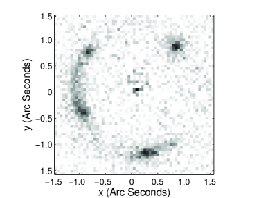
Figure 1.— The HST/WFPC2 image of the optical Einstein ring 0047-2808 employed in this study. The image has a side length of 3.05 arcseconds and comprises of 61x61 pixels. As noted in the text, the light distribution of the foreground galaxy has been subtracted (see Wayth et al., 2005); this foreground light distribution increases the noise in the central regions of this image.

As with Wayth et al. (2005), a noise frame covering the same region and including the various noise components (such as that from the light distribution of the lensing galaxy) was also employed. It should be noted that this study did not recreate the image dithering procedure that was undertaken with the observed system, rather it is assumed that the image presented in Figure 1 is a true representation of this lensing system at a resolution of 0.05 arcseconds. To this end, the point spread function was generated with the TinyTim algorithm to match this resolution scale (Krist, 1995). Although in reality the noise values between neighbouring pixels are correlated, we will use an uncorrelated likelihood function, which is computationally much more managable and will lead to slightly more conservative results.

3. approach

3.1. Parameter Estimation

The basis of our method was presented in BL06. For a more general introduction to Bayesian methods, including Markov Chain Monte Carlo techniques, see the textbook by Gregory (2005). Assuming a particular form for the lens model, and background information or assumptions $I$, we write down the joint probability distribution for the lens and source parameters (denoted collectively by $L$ and $s$ respectively) given the data $D$ and the prior information and assumptions $I$:

$$p(SL|DI)=\frac{p(SL|I)p(D|SLI)}{p(D|I)}$$ (1)

The denominator does not depend on the source and lens parameters, so is part of the normalisation constant for the joint probability distribution. The first factor in the numerator is the joint prior probability density of the lens and source parameters, and the second factor is the likelihood function (probability density of the data that was actually observed, given the parameters). Commonly, the source is pixellated into $m$ pixels and is described by a vector $\mathbf{s}$ of pixel intensities, and the observed image is also pixellated (with $n$ pixels), and is represented by a vector $\mathbf{O}$. In this case the image predicted by a source is calculated by a matrix multiplication: $\mathbf{I=Ls}$. The matrix $\mathbf{L}$ depends on the lens parameters $L$ and the point spread function. Since it is always possible that the noise level values {$\sigma_{i}$} are not completely reliable, we also introduced an extra noise parameter $\sigma$, to be estimated from the data (Gregory, 2005). If a good fit is possible with our model, $\sigma$ will be estimated to be small. If a good fit is not possible, $\sigma$ will be estimated to be large, and the uncertainties in all other inferred parameters will also be increased. Thus, we can use the inferred value of $\sigma$ as a kind of alternative-free test of whether our lens model is adequate. Under the usual assumptions (a Gaussian probability distribution for the error in each pixel of the image, and logical independence of the prior information about the lens and the source), we have the PDF

$$p(\mathbf{s}L\sigma|DI) \propto p(\mathbf{s}|I)p(L|I)p(\sigma|I)p(\mathbf{O}|{s}L\sigma I)$$

$$\propto p(\mathbf{s}|I)p(L|I)p(\sigma|I)\times$$

$$\left[\prod_{i=1}^{n}\frac{1}{\sqrt{\sigma^{2}+\sigma_{i}^{2}}}\right]e^{-\frac{1}{2}\sum_{i=1}^{n}\frac{(O_{i}-\sum_{j=1}^{m}L_{ij}s_{j})^{2}}{\sigma^{2}+\sigma_{i}^{2}}}$$ (2)

where the right hand side depends on the lens parameters through the matrix $\mathbf{L}$ in some complicated nonlinear fashion. Therefore, there is no hope of finding marginal distributions analytically, so we will use a Markov Chain Monte Carlo algorithm to generate random samples from this posterior distribution.

3.2. Lens Model

For its convenient properties, we chose an softened power-law elliptical potential (SPEP) for the lens model (Barkana, 1998). Elliptical potentials have the advantage of faster computation of the deflection angles than for elliptical projected mass distributions, and great flexibility in the range of possible lenses is achievable with a handful of parameters. Hopefully, this flexibility is sufficient to ensure that we won’t make any overconfident conclusions caused by the fact that real lenses are not exactly described by some parametric model. The primary reason for choosing this model was computational speed, which is an important consideration because our MCMC algorithm requires a lot of likelihood evaluations.

The 2-D lensing potential we used was

$$\phi(x,y)=\frac{b}{\gamma}R^{\gamma}$$ (3)

where

$$R=\sqrt{r_{c}^{2}+x^{2}q+y^{2}/q}$$ (4)

The gradient of $\phi$ gives the deflection angles as

$$\alpha_{x}(x,y)=\frac{\partial\phi}{\partial x}=(bqx)R^{\gamma-2}$$ (5)

$$\alpha_{y}(x,y)=\frac{\partial\phi}{\partial y}=(by/q)R^{\gamma-2}$$ (6)

The parameter $b$ is the overall strength of the lens, and $q$ is the ratio of the ellipse’s major and minor axes. $q\sim 1$ indicates an approximately circularly symmetric lens. Furthermore, $(x,y)$ is position in the lens plane, in a coordinate system aligned with the lens and centred at the centre of the lens. Thus, in fitting the lens to an observed image, we have 7 free parameters: $b$, $q$, $(x_{c},y_{c})$ (the position of the centre of the lens), $\gamma$, a slope parameter, the core radius $r_{c}$ and $\theta$, the angle of orientation of the lens mass distribution with respect to the axes defined by the image. If $q=1$,$\gamma=1$ and $r_{c}=0$, this model reduces to the common isothermal sphere model, for which $b$ is the Einstein Radius. It is not clear whether $(x_{c},y_{c})$ were considered known a priori in previous investigations; here we will consider them partially known by assigning a weakly informative prior probability density. Using the scaled lens equation with source and image plane positions measured in arc seconds corresponds to a choice of the units of mass, as being that which would make the Einstein radius equal to 1 arc second.

It is usually the case that an image can be fitted with a variety of differently parametrized lens models. However, for most purposes we are more interested in the values of the parameters themselves (e.g. how much mass is there, how elliptical is the density profile, is it aligned with the light profile of the lensing galaxy, etc) and little would be gained by comparing different choices for the parameterisation of the mass model. However, we suspect that, if very high resolution images were available, simple lens models would be inadequate and we would need to use a nonparametric mass model, similar to that used by Marshall (2005) for weak lensing. It is difficult to determine at what point this would be neceessary, however, if our “extra noise” parameter $\sigma$ was inferred to be large then this would be a definite indication that a different mass model is required.

3.3. Lens Parameter Priors

In order for the problem to have a definite solution, we need to introduce prior probability distributions for the parameters of the lens model, to describe our prior knowledge or ignorance about their values. In principle, we could consider the image of the foreground galaxy as providing prior information, however we did not carry out any sophisticated analysis along these lines, because the final results depend only very weakly on the specific choice of functions. The prior probability densities we used for each parameter are shown in Table 1. These are only intended to capture vague prior information about the range of values that the parameter could plausibly take. For the position of the centre of the lens model, we assumed this was near the centre of the light profile of the foreground galaxy, but the large prior standard deviation of 0.2 means that this is a weak assumption.

Table 1Prior probability densities for the lens model parameters, and also the extra noise parameter $\sigma$.

Parameter	Prior Distribution
$b$	Exponential, mean 1”1-γ
$q$	Normal, mean 1”, SD 0.2”
$r_{c}$	Exponential, mean 0.5”
$\gamma$	Normal, mean 1, SD 0.2
$x_{c}$	Normal, mean 0.092”, SD 0.2”
$y_{c}$	Normal, mean 0.164”, SD 0.2”
$\theta$	Uniform, between 0 and $2\pi$
$\sigma$	Jeffreys’ uninformative prior $\propto 1/\sigma$

3.4. Source Prior

Since the source may have complex structure, we need to introduce enough pixels to capture this in detail. We chose to use a 48x48 pixel grid to represent the source. The range of the source plane that was covered was 0.6 arc seconds across, so the resolution over the source plane was a factor of 4 greater than the resolution of the image. If the image strongly constrains part of the source, this will be reflected in the posterior samples. This may or may not occur (depending on the quality of the data), but using large numbers of pixels at least keeps the option open. Since we are not using an optimisation based approach, overfitting does not occur.

In BL06, we discussed the shortcomings of regularization based priors for astronomy, and suggested simple priors which should be more realistic. In this paper, we use a prior which is somewhat more complex than that described in BL06. The prior probability distribution describing the range of source models which we consider plausible was constructed as follows. Since the source is mostly blank, rather than trying to infer each source pixel value directly, we imagine that the source is generated by “monkeys” throwing $N$ “atoms” of intensity onto the (initially blank) source plane. Each atom has four attributes: An intensity $B$, a discrete position $(i,j)$, indicating which pixel the atom landed in, and a width parameter. The prior probability density of the intensity $B$ of an atom is taken as exponential with mean $\mu$ (chosen to match the typical brightness scale of the image), and the prior distribution of the discrete position $(i,j)$ of each atom is uniform. This is similar to the Massive Inference prior suggested by Skilling (1998) for positive, additive distributions such as surface brightness distributions. It has the desirable property that the prior probability distribution for the amount of integrated light over any macroscopic region R of the source plane is independent of how we choose to subdivide that region into pixels.

Allowing the atoms to have variable size allows us to reconstruct plausible astrophysical sources with only a small number of atoms, negating the problems caused by an entropic prior, which tends to make the reconstructed sky too bright, possibly also causing other parameters to be inferred incorrectly (BL06). MEM may be suitable for photographs, but for astronomy, MassInf is more appropriate. Also, there is some prior expectation that the source should contain correlations, so that bright pixels are more likely to be near other bright pixels. To take this into account, we allowed three different types of atoms to make up the source - single pixel sized atoms, and two “fuzzier” types of atoms that spread light over several pixels. The effect of this variable atom size is to reduce the impact of our particular choice of pixellation scale, by allowing finer structure in those parts of the source where it is justified by the data. We chose to discretize into three distinct types of atom to reduce computational load, because if we had allowed the atom width to be a continuous variable it would have taken much more computation to produce the pixellated source for lensing.

In our MCMC simulations, we modified the source by manipulating the atoms (positions, intensities, widths, and number) directly, rather than by modifying source pixel values directly. This helps, because an increased acceptance rate can be achieved using proposal transitions that move an atom from one pixel to its neighbour; since this will only have a slight effect on the predicted image, the acceptance probability will be fairly high. Also, most proposal moves for the Metropolis algorithm will be concentrated around modifying the bright parts of the source (where the atoms are), so little time is wasted adjusting pixels where the source is mostly blank.

3.5. MCMC Sampling

A feature of the lens inversion problem is the fact that it is much faster (by a factor of $\sim$ 50) to compute the image for a new source, with a fixed lens model, than it is to compute the image for a new lens parameter set. This is because, to calculate the image after modifying only the source, a matrix multiplication (by a sparse matrix) is required. However, to calculate the new image after a change in the lens parameter values requires that we calculate the sparse lensing/blurring matrix $\mathbf{L}$, which requires a large ray tracing calculation, firing 100 rays per pixel in order to get an accurate approximation to the lensing matrix. A modified Metropolis method has been developed by Neal (2004) which is designed to improve the sampling when some variables are “slow” and others “fast”, so we implemented this in our code. Parallel tempering (Gregory, 2005) was also used to ensure efficient exploration of the parameter space. The MCMC simulation was run several times with different random number seeds, in order to check convergence. The results were deemed to be reliable enough if the variance of the error bars returned was significantly less than their size, which was the case.

4. Results

4.1. Source

Figure 2 shows two results from the MCMC simulation (i.e. two samples from the posterior distribution). The lensed and blurred images are also shown, and the residuals between the images and the observed image are consistent with pure noise, in terms of $\chi^{2}$. If the number of degrees of freedom (data points minus effective number of free parameters) was well defined, the image would not match the observed one to the extent that a frequentist goodness of fit test would demand. However, since we are not using optimization, these common tests do not apply.

Individual reconstructions tend to have their flux concentrated into a small number of pixels (across a physical length scale of 1-2 kpc), but the reliable conclusions are the ones which are reproduced across most of the sources in the sample. Nine more samples are shown in Figure 3.

In Figure 4, the posterior mean source is displayed. This may be taken as a final estimate of the source (if a single estimate is required), and when this is lensed, it is consistent with the image to within the size of the noise error bars. The posterior samples and the mean source both show strong evidence for complex structure in the upper right region of the source, with a component protruding out at right angles to the main component. Other authors have suggested that this may be a system of interacting galaxies (Dye & Warren, 2005; Wayth et al., 2005). This feature is present in the vast majority of the source samples, indicating that the evidence for two components is strong.

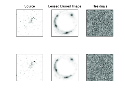
Figure 2.— Two samples from the posterior distribution of sources, along with their lensed blurred images and the normalized residuals between the model and the data. The source plane is 0.6 arc seconds across, corresponding to a physical length scale of $\sim$ 7 kpc.

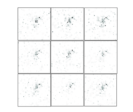
Figure 3.— More sample sources from the posterior distribution. The diversity across the samples is an indication of the uncertainty that we have about the nature of the source.

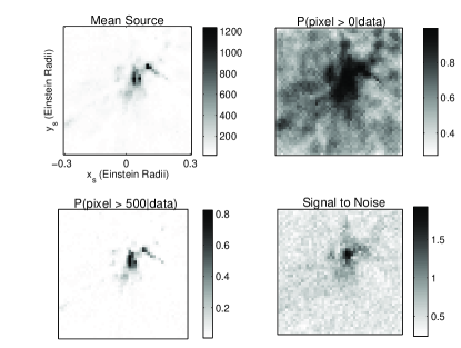
Figure 4.— The mean source reconstruction (top left) serves as a final estimate of the source, with the two components clearly visible. The next two panels are the marginal posterior probabilities that each pixel is greater than zero, and greater than 500 respectively, and so quantify the amount of evidence for each part of the source. The bottom right plot is the ratio of the mean flux to the standard deviation, showing that we have the most information about the brightest parts of the source.

In principle, to decide whether or not this is a double source, we should measure the posterior probability that the source is double, by counting the fraction of samples which are double. But this is problematic - since we are using a nonparametric source model, it becomes hard to define what is meant by a double source. Despite this difficulty, the question can be answered by simply observing the sequence of source models and noting that the component at right angles to the main light source is persistent across the vast majority of the posterior samples (Figure 3), indicating a robust conclusion. This is also demonstrated by the significance maps in Figure 4.

In the primary component of the mean source map, some substructure is visible, suggesting that we may have resolved extra detail in the core of this galaxy. However, the low value of the signal to noise ratio ($\sim$ 1) casts doubt on this conclusion. Individual pixels are highly underconstrained in our approach, it is the integral properties of the source that are robustly measured. As a check, we calculated the posterior probability that both pixels (20,27) and (20,29) are brighter than pixel (20,28), and found this probability to be 0.48, and hence that this question cannot be answered with the current data. Also, there is some weak evidence for more patches of the light to the left of the primary component, but better data would be required to firmly establish this.

In Figure 5, the two possible components of the mean source are plotted separately, and the images of them are shown. The first component contributes to three of the images, but causes a large extended region of light on the left of the image. The second component is needed in order to explain the additional, more concentrated component of the leftmost image, as well as the presence of the fourth image. A similar conclusion was reached by Wayth et al. (2005) and Dye & Warren (2005), however, our simulations have found evidence for a structure that is long and narrow, on the scale of the pixel size that we have used. Since other authors have used larger pixels, they have found that the best fitting source is a binary source in which both components are blobby, whereas our results suggest a needle-like structure for the second component, with a width of $\sim$ 200 pc.

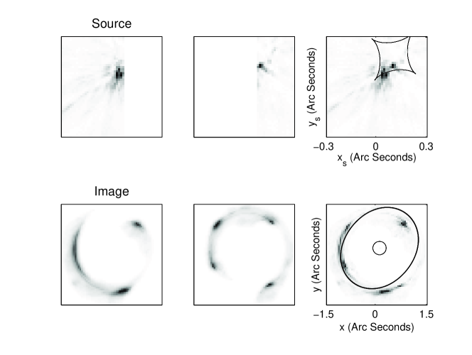
Figure 5.— The two components of the reconstructed source, plotted separately to show how they contribute to the image. On the right, the estimated source and lensed (not blurred) image are plotted along with the caustics and critical lines for the best fitting lens model.

4.2. Lens Parameters

The estimates of the lens model parameters are shown in Table 2 (the units, where appropriate, are arcseconds, except for $\theta$ which is in radians). These estimates are similar to those found by Wayth et al. (2005) using a similar (PIEP) lens model, but our uncertainties are greater, by a factor of $\sim$ 1-4.

There are several factors contributing to this increased uncertainty. One is due to the fact that we have used more pixels than others, making weaker a priori assumptions about the source’s structure. We have also used a different, more reasonable prior for the source, taking into account the fact that astronomical sources are usually localized bright patches with a dark background. Regularization based priors (Suyu et al., 2006) may not take this into account.

Another possible cause for the increased uncertainty is the approximations that have previously been used, such as a Gaussian approximation to the posterior PDF about its peak. This is typically a good approximation if the data constrains the parameters very well, but this is not usually the case with “non-parametric” (actually many-parametric) reconstructions. Finally, we did not fix the centre of the lens mass distribution at a particular point, but included this as an extra pair of parameters to be inferred from the image, and also included the $\gamma$ and $r_{c}$ parameters.

To infer any properties of this lensing system (with corresponding uncertainties), all that is required is to calculate the desired property for all of the posterior samples, and observe the diversity of the answers. As an example, we were able to measure the total magnification of this system, defined as the flux in the image divided by the flux of the source; this value was found to be 17.9 $\pm$ 1.7, further demonstrating the value of lensing for investigations of high redshift galaxies.

The lens mass distribution was found to be slightly elliptical, with q = 0.932 $\pm$ 0.006, and the angle of orientation of the lens (which can be seen from the orientation of the critical curves in Figure 5) is close to that of the subtracted foreground galaxy (see Wayth et al., 2005).

From these results we can also estimate the total mass contained within the image. We defined a circle of radius 1.2 arc seconds centred in the middle of the image and integrated the density (proportional to the Laplacian of the lensing potential) within this ring, for each lens parameter set. Given our assumptions, the mass contained within the ring was found to be (2.91$\pm$0.01)$\times$10¹¹ M_☉, in agreement with the value reported by Koopmans & Treu (2003), who found a slightly lower value but also used a ring of slightly smaller radius.

Table 2Results for lens model parameters. Where appropriate, the units are arc seconds, except for $\theta$, which is in radians. The values found by Wayth et al. (2005) for the similar PIEP model are also shown. For the $\gamma$ parameter, the quoted value from Wayth et al. (2005) was from a softened power-law elliptical mass density model.

Parameter	Value	Wayth et al. (2005)
$b$	1.177 $\pm$ 0.016 (”1-γ)	1.170 $\pm$ 0.004
$q$	0.932 $\pm$ 0.006	0.917 $\pm$ 0.004
$r_{c}$	0.09 $\pm$ 0.07	N/A
$\gamma$	1.04 $\pm$ 0.06	1.08 $\pm$ 0.03
$x_{c}$	0.107 $\pm$ 0.006	N/A
$y_{c}$	0.176 $\pm$ 0.008	N/A
$\theta$	2.245 $\pm$ 0.009	2.247 $\pm$ 0.01
$\sigma$	Negligible	N/A

5. Conclusions

In this paper, we have presented an analysis of the HST image of the Einstein ring 0047-2808 using a Bayesian procedure. Most of the results are qualitatively consistent with previous work, leading us to conclude that the various different methods available for reconstructing gravitational lens systems all give satisfactory results for this system, despite the disagreement about the uncertainties in the parameter estimates. However, this may not always be the case with other data sets (see Gregory, 2005, for an example). However, our use of smaller pixels and a more reasonable prior for the source has allowed us to reconstruct the source with a greater resolution than has been possible with other methods. As a result, we have found that the second component of the source is not just a single patch of light, but has a narrow structure protruding from it; given structure formation in $\Lambda$CDM cosmologies, we should expect such objects in the early universe to show significant substructures indicative of major mergers and accretion.

Discovered in continuum radio sources (Hewitt et al., 1988), the number, diversity and observational detail of Einstein rings has continued to grow (e.g. Cohen et al., 2003; Treu & Koopmans, 2003; Carilli et al., 2003). Furthermore, optical Einstein rings should be uncovered in a upcoming surveys (Miralda-Escude & Lehar, 1992), particularly the SLACS survey (Bolton et al., 2006), and the number of cases is steadily increasing (Sluse et al., 2003; Cabanac et al., 2005). Hence it is vital that progress is made in developing and understanding optimal and reliable methods for analyzing them. Model selection will probably play an important role in this area in the future (Suyu et al., 2006), however we doubt that it will be useful to compare the evidence for one ad-hoc regularization formula against another, when it is known in advance that neither of them accurately describe the prior information that is available. Despite these concerns, the level of qualitative agreement between the results presented in this paper and in others show that these debates may only be of minor importance in practice.

References

- Barkana (1998) Barkana R., 1998, ApJ, 502, 531
- Bolton et al. (2006) Bolton, A. S., Burles, S., Koopmans, L. V. E., Treu, T., & Moustakas, L. A. 2006, ApJ, 638, 703
- Brewer & Lewis (2005) Brewer B. J., Lewis G. F., 2005, PASA, 22, 128
- Brewer & Lewis (2006) Brewer, B. J., Lewis, G. F., 2006, ApJ, 637, 608
- Cabanac et al. (2005) Cabanac R. A., Valls-Gabaud D., Jaunsen A. O., Lidman C., Jerjen H., 2005, A&A, 436, L21
- Carilli et al. (2003) Carilli, C. L., Lewis, G. F., Djorgovski, S. G., Mahabal, A., Cox, P., Bertoldi, F., & Omont, A. 2003, Science, 300, 773
- Cohen et al. (2003) Cohen, J. G., Lawrence, C. R., & Blandford, R. D. 2003, ApJ, 583, 67
- Dye & Warren (2005) Dye S., Warren S. J., 2005, ApJ, 623, 31
- Futamase & Hamaya (1999) Futamase T., Hamaya T., 1999, PThPh, 102, 1037
- Gregory (2005) Gregory P. C., 2005, ApJ, 631, 1198
- Gregory (2005) Gregory P. C., 2005, Bayesian Logical Data Analysis for the Physical Sciences: A Comparative Approach with Mathematica Support (Cambridge: Cambridge Univ. Press)
- Hewitt et al. (1988) Hewitt, J. N., Turner, E. L., Schneider, D. P., Burke, B. F., & Langston, G. I. 1988, Nature, 333, 537
- Kochanek et al. (1989) Kochanek C. S., Blandford R. D., Lawrence C. R., Narayan R., 1989, MNRAS, 238, 43
- Kochanek, Keeton, & McLeod (2001) Kochanek C. S., Keeton C. R., McLeod B. A., 2001, ApJ, 547, 50
- Kochanek & Wambsganss (2004) Kochanek, C.S., Schneider, P., Wambsganss, J., 2004, Part 2 of Gravitational Lensing: Strong, Weak & Micro, Proceedings of the 33rd Saas-Fee Advanced Course, G. Meylan, P. Jetzer & P. North, eds. (Springer-Verlag: Berlin)
- Koopmans & Treu (2003) Koopmans L. V. E., Treu T., 2003, ApJ, 583, 606
- Krist (1995) Krist J., 1995, in Shaw R. A., Payne H. E., Hayes J. J. E., eds, ASP Conf. Ser. Vol. 77, Astronomical Data Analysis Software and Systems IV. Astron. Soc. Pac., San Francisco, p. 349
- Marshall (2005) Marshall, P., 2005, astro-ph/0511287
- Miralda-Escude & Lehar (1992) Miralda-Escude J., Lehar J., 1992, MNRAS, 259, 31P
- Neal (2004) Neal, R. M., 2004, Taking Bigger Metropolis Steps by Dragging Fast Variables, Technical Report No. 0411, Dept. of Statistics, University of Toronto. arXiv:math/0502099
- Schneider, Ehlers, & Falco (1992) Schneider P., Ehlers J., Falco E. E., 1992, Gravitational Lenses, (Berlin: Springer)
- Skilling (1998) Skilling J., 1998, Massive Inference and Maximum Entropy, in Maximum Entropy and Bayesian Methods, Kluwer Academic Publishers, Dordrecht/Boston/London p.14
- Sluse et al. (2003) Sluse, D., et al. 2003, A&A, 406, L43
- Suyu et al. (2006) Suyu S. H., Marshall P. J., Hobson M. P., Blandford, R. D., 2006, astro-ph/0601493
- Treu & Koopmans (2003) Treu, T., & Koopmans, L. V. E. 2003, MNRAS, 343, L29
- Warren & Dye (2003) Warren S. J., Dye S., 2003, ApJ, 590, 673
- Warren et al. (1998) Warren S. J., Iovino A., Hewett P. C., Shaver P. A., 1998, MNRAS, 299, 1215
- Warren et al. (1996) Warren S. J., Hewett P. C., Lewis G. F., Moller P., Iovino A., Shaver P. A., 1996, MNRAS, 278, 139
- Warren et al. (1999) Warren S. J., Lewis G. F., Hewett P. C., Møller P., Shaver P., Iovino A., 1999, A&A, 343, L35
- Wayth et al. (2005) Wayth R. B., Warren S. J., Lewis G. F., Hewett P. C., 2005, MNRAS, 360, 1333