New evidence for a linear colour–magnitude relation and a single Schechter function for red galaxies in a nearby cluster of galaxies down to $\mn@boldsymbol{M^{*}+8}$

Abstract

The colour and luminosity distributions of red galaxies in the cluster Abell 1185 ($z=0.0325$) were studied down to $M^{*}+8$ in the $B$, $V$ and $R$ bands. The colour–magnitude (hereafter CM) relation is linear without evidence for a significant bending down to absolute magnitudes which are seldom probed in literature ($M_{R}=-12.5$ mag). The CM relation is thin ($\pm 0.04$ mag) and its thickness is quite independent from the magnitude. The luminosity function of red galaxies in Abell 1185 is adequately described by a Schechter function, with a characteristic magnitude and a faint end slope that also well describe the LF of red galaxies in other clusters. There is no passband dependency of the LF shape other than an obvious $M^{*}$ shift due to the colour of the considered population. Finally, we conclude that, based on colours and luminosity, red galaxies form an homogeneous population over four decades in stellar mass, providing a second evidence against faint red galaxies being a recent cluster population.

1 Introduction

One of the major problems facing models of galaxy formation is why cold dark matter models predict a larger number of low-mass galaxies than observed. Today, extremely faint ($M\gg M^{*}+5$ mag) galaxies are still a poorly studied population because they are difficult to find and, once found, the measurement of their properties is not trivial since the measured properties are usually strongly affected by selection effects. Thus, understanding the properties of the lowest luminosity galaxies, which are presumably also very low mass, might shed light on some of the unsolved questions related to the production of galaxies in low-mass halos.

The bulk of the observational work on low-luminosity galaxies is limited to clusters environment. The pioneering work by Visvanathan & Sandage (1977) presents the colour-magnitude relation over an eight magnitude range, although the very large majority of the data is relevant to the brightest four magnitudes. Secker et al. (1997) reports that the colour-magnitude relation (also known as the red sequence) is linear in the Coma cluster over a seven magnitude range, i.e. down to $M_{R}=-15.0$ mag. Conselice et al. (2002) confirms that galaxies in the first four magnitudes of the Perseus clusters obey to the usual colour–magnitude relation (e.g. Bower, Lucey & Ellis 1992), but faint candidate members of the cluster tend to depart from the colour of the red sequence, being bluer or redder. The scatter around the red sequence is small ($\sigma\approx 0.07$ mag) down to $M_{R}\sim-17$ mag, but rises to $\sigma\approx 0.5$ mag at $M_{R}\sim-14$ mag. Instead, Evans et al. (1990) found that the fainter Fornax galaxies become redder, not bluer. Therefore, it is unclear what is the shape of the red sequence at faint magnitudes and if it is universal or if it changes from cluster to cluster.

In other environments, information is even scarcer. In the review article by Mateo (1998) on dwarf galaxies in the local group, the colour-magnitude relation includes about 30 galaxies in the range $-22<V<-11$ mag. Blanton et al. (2005) derived luminosity and colour distributions of faint galaxies in the local universe for a flux and surface brightness limited sample. However, it is unclear how much their results are affected by the fact that they assume no environment dependence and a uniform spatial distribution of the studied sample, and later on, the distributions were claimed environmental-dependent and the sample clustered (see Andreon, Punzi & Grado 2005 for a discussion).

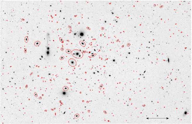
Figure 1: (Compressed) image of the studied field in the $R$ band, with red galaxies (members and background) marked with an ellipse. North is up and east is to the left. The field of view is $42\times 28$ arcmin².

In this paper, we report results about a volume complete sample of galaxies in a nearby cluster of galaxy, Abell 1185. Our data are deep enough to reveal extremely faint objects, allowing us to investigate the properties of red galaxies over a nine magnitude range.

Abell 1185, a cluster of richness one class (Abell 1858), has a redshift $cz=9800$ km s^-1 and a velocity dispersion of $\sigma_{v}=740\pm 60$ km s^-1 (Mahdavi et al. 1996), and an X-ray luminosity of $L_{X}$(0.5-3 keV) $=1.6\ 10^{43}$ $h_{50}^{-1}$ ergs s^-1 (Jones & Forman 1984).

For the Abell 1185 cluster, we adopt a distance modulus of 35.7 mag ($H_{0}=70$ km s^-1 Mpc^-1, $z=0.0325$).

2 The data and data reduction

Abell 1185 observations and data reduction follow closely a similar analysis performed on the Coma clusters (Andreon & Cuillandre 1999, AC02 hereafter), to which we defer for details.

$B$, $V$ and $R$ cluster observations were taken on January 31th, 2003 in photometric conditions, with the CFH12K camera (Cuillandre et al. 2000) at the Canada–France–Hawaii Telescope (CFHT) prime focus in photometric conditions. CFH12K is a 12,288 $\times$ 8,192 pixel CCD mosaic camera, with a 42 $\times$ 28 arcmin² field of view and a pixel size of 0.206 arcsec. Five dithered images per filter were taken, pre-reduced (overscan, bias, dark and flat–field) and then optimally stacked. The total exposure time was 1500, 1200 and 900 s in $B$, $V$ and $R$, respectively. Seeing in the combined images is 1.2 to 1.3 arcsec FWHM. The CFHT CCD mosaic data reduction package FLIPS (Magnier & Cuillandre 2004) was used. After discarding areas noisier than average (gaps between CCDs, borders, regions near bright stars, etc.), the usable area is 0.263 deg², or 1.3 Mpc² at the cluster redshift. Images were calibrated in the Bessel–Cousin–Landolt system through the observation of photometric standard star fields listed in Landolt (1992).

Figure 1 shows an highly compressed $R$ band image of Abell 1185.

In this work, interloper galaxies are statistically removed. This requires that the cluster and the control field images share the same photometric system: in presence of colour mismatches, which often arise from using data coming from different telescopes/instruments/filters, the background contribution is usually assumed to be perfectly removed whereas instead it leaves some residuals, biasing the LF and colour measurements. Our control field has been published and described in McCracken et al. (2003). These images were taken using the very same $B$, $V$ and $R$ filters, telescope and instrument used for the present study; they were reduced by the same software, calibrated in the same photometric system by the same standard fields, hence assuring a perfect homogeneity between the two data sets. The control field is much deeper than the cluster observations, and therefore we consider only the magnitude range that matches the cluster images. Even if our data are homogeneous, we nevertheless verified that cluster and control field images share the same locus of stars, in the $V-R$ vs $B-V$ colours (e.g. as in Fig 1 of Andreon, Lovo, & Iovino 2004), and in the $(V-R)-(B-V)$ vs $B-V$, in order to enhance the visibility of any mismatch. As a further check, we compared the density distribution of galaxies in the $V-R$ vs $B-V$ plane, and did not detect any colour offsets between the cluster and the control field images.

Objects are detected using SExtractor (Bertin & Arnouts 1996), using a isophotal threshold of 26.0, 25.5, 24.5 in $B$, $V$ and $R$, respectively, corresponding to a threshold of $\approx 2\sigma$ of the sky in the cluster images, and more than 5 $\sigma$ in the control field images.

In this paper, we adopt SExtractor isophotal corrected magnitudes as a proxy for “total” magnitudes; we do not choose Kron magnitudes because of their flip–flopping nature described in Andreon, Punzi & Grado (2005, APG hereafter). Completeness is measured as the magnitude of the brightest low surface brightness galaxy of the faintest detectable central surface brightness, as described in Garilli, Maccagni & Andreon (1999). Cluster data are complete down to $B=24.0$, $V=23.8$ and $R=22.7$ mag, but further clipped to a brighter magnitude range ($B=23.25$ or $V=22.45$ or $R=22.0$ mag, depending on the measured quantity), in order to be nearly 100% complete in colour, and in order to reduce the Eddington bias (see sec 3.5.2 in AC02 for details). Fundamentally, from more than 10,000-20,000 detections in the cluster line of sight, we select the brightest 2,000 galaxies with the rationale of keeping the best data.

Stars are discarded by combining the probabilities derived by SExtractor in the three filters. We conservatively keep a high threshold, rejecting “sure stars” only ($class_{star}>0.95$) in order not to exclude the compact galaxies, while leaving some residual stellar contamination in the sample: it (as well as the contamination caused by background galaxies) is dealt with statistically later on. Most galaxies are easily classified as extended sources in the magnitude range of our interest. Very compact galaxies, such as NGC 4486B or M 32, are however easily misclassified as stars at the Fornax (Drinkwater et al. 1999) and Coma (AC02) clusters distances, but they represent a minority population (Drinkwater et al. 1999, AC02). Finally, blends of globular clusters (GCs) that are not resolved in individual components due to seeing, and look like dwarf galaxies on our ground-based images, are expected, but from what is observed in the Coma cluster (AC02), the GCs blends start to contaminate galaxy counts at fainter magnitudes than the range probed in this work.

3 Results

3.1 Exploring the colour-colour-magnitude data cube

Let us explore the colour-colour-magnitude cube by observing it through different projections.

Figure 2 is a projection of the colour-colour-magnitude cube that aligns the observer’s eye along the colour–magnitude (hereafter CM) relation. The projection is along an axis slightly tilted with magnitude, with slopes $0.2/6$ and $0.1/6$ mag in $B-V$ and $V-R$, respectively (these are logically the slopes of the colour–magnitude relations in the two colours). Technical details about the way the CM slope is determined are given in the appendix. Colours are corrected to $R=20$ mag for the slope of colour–magnitude. The left and right panels refer to galaxies in the cluster and in the control field lines of sight, respectively. The number density distribution of control field galaxies (right panel) shows a shallow gradient from bottom-right to top-left, more evident when the whole control field data set is plotted (in the figure, only one galaxy out of 4.7 is plotted to account for differences in the surveyed area and to make the two panels easy to compare by eye). Superimposed to the shallow gradient, the colour distribution of galaxies in the cluster line of sight (left panel) shows a clear excess at $B-V=0.98$, $V-R=0.62$ mag, marked with a circle in the figure.

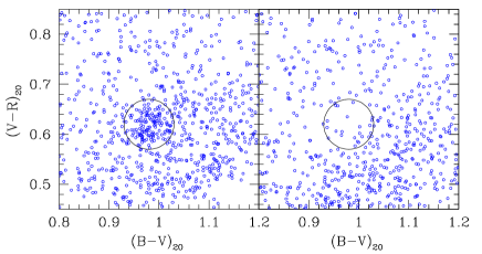
Figure 2: Colour-colour distribution of galaxies in the cluster (left panel) and control field (right panel) lines of sight. An obvious overdensity is seen at the colour of the red sequence ($B-V=0.98$, $V-R=0.62$ mag). Colours are corrected to $R=20$ mag for the colour–magnitude effect. In the right panel, we randomly plot 1 out of 4.7 galaxies from the control field galaxies, in order to account for differences in surveyed areas.

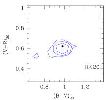
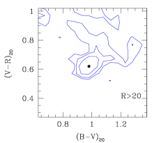
Figure 3: Background subtracted number density distribution of Abell 1185 members in the colour–colour plane. The left and right panels show the distribution of $R<20$ mag ($M_{R}=-15.7$ mag) and $R>20$ mag, respectively. Contours are draw to levels set at 1/2, 1/4 and 1/8 of the peak value. The extension in the right panel toward red colours of the lowest contour has $S/N\sim 1$.

Figure 3 shows the colour distribution, binned in colour bins and background subtracted using our control field. The direction that point to the observer is now the number density of Abell 1185 members of a given colour. The two panels display the result for galaxies brighter (left panel) and fainter (right panel) than $R=20$ mag ($M_{R}=-15.7$ mag). A clear peak at the colour of the colour-magnitude relation is seen in both panels. The peaks are narrow: they have a width of $\pm 0.04$ mag (see appendix), implying that the thickness of the red sequence is small. In Figure 3, the shown distributions are the observed distributions convolved by a $0.1$ mag top-hat kernel. The two peaks are almost centered at the same colour ($B-V=0.98$, $V-R=0.62$ mag), shown as points in the figure. In the left panel there is an insignificant 0.02 mag offset in $V-R$, 1/5 of the width of the color bin. This implies that the colour-magnitude relation does not deviate from linearity at faint magnitudes. A 0.1 mag shift would be very easily identified in the above plot.

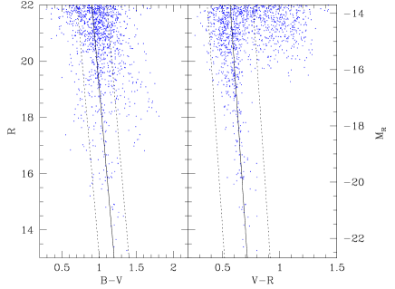
Figure 4: Colour–magnitude distribution of galaxies in the Abell 1185 line of sight. In each panel are plotted galaxies within 0.2 mag from the red sequence in the other colour. Based on the control field images, we estimate that only one in five of the plotted galaxies is a cluster member.

Figure 3 also shows that Abell 1185 has a low fraction of blue galaxies in the observed portion (our images sample about half of the cluster virial radius, which was computed from the cluster velocity dispersion using equation 1 of Andreon et al. 2006): the peak does not show any large extension toward bluer (say, 0.2 mag or more) colours. The S/N of the top–right part of lowest contours in right panel of Fig 3 is $\sim 1$. Therefore, the extension toward red colours of the $R>20$ distribution is hardly significant at all.

Figure 4 shows the distribution of galaxies in the colour–magnitude plane of galaxies in the Abell 1185 line of sight. Each panel shows galaxies falling in a plane of the colour-colour-magnitude cube of thickness 0.4 mag in the other colour, in order to reduce the contamination by background galaxies. Because the spread around the red sequence is five times smaller (see Figure 3 and Appendix), the 0.4 (i.e. $\pm 0.2$) mag thickness is wide enough to avoid selectively removing any red sequence galaxy, and therefore does not bias the slope of the red sequence. After the above selection, we known from control field data that only one in five of the plotted galaxies is a cluster member. The colour–magnitude relation in $B-V$ and $V-R$ vs. $R$ are outstanding for galaxies brighter than $R=20$ or $21$ mag. At fainter magnitudes the background contribution makes the colour–magnitude relation difficult to disentangle. Figure 3 shows, however, that at $R>20$ the colour–magnitude relation does not bend.

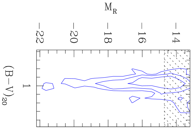
Figure 5: Background subtracted number density distribution of Abell 1185 members in the colour–magnitude plane. Each panel shows galaxies falling in a plane of the colour-colour-magnitude cube of thickness 0.4 mag in the other colour, in order to reduce the contamination by background galaxies.

Figure 5 shows the number density distribution in the colour–magnitude plane after background subtraction. In order to reduce the noise due to background fluctuations, we considered only galaxies within $\pm 0.1$ mag in $V-R$ from the red sequence, which is a sensible choice given the small $V-R$ scatter of red galaxies. As in Figure 2 and 3, we have magnitude–corrected colours to align the $R$ magnitude with one of the figure axis. As in Figure 3, the data are convolved (binned) by a top-hat function of $\pm 0.05$ mag width in colour. The shaded region is affected by borders effects. The figure confirms the linearity of the red sequence and its almost constant width.

The interpretation of these results is deferred to Sec. 4.4

We define as red galaxies the objects having colours within 0.1 mag from both colour–magnitude relations. Such a definition leaves intact the peak of the colour distribution centered on red galaxies (see in particular Figure 3) and leaves room for objects scattered off from the red sequence by (our small) photometric colours.

The sample of red galaxies turns out to be composed of about 180 members plus a similar number of background galaxies. As a further check, we consider a second sample, relaxing the tightness of the colour constraint from $0.1$ to $0.2$ mag. The number of red galaxies remains unchanged, but the number of background galaxies grows by more than a factor four!

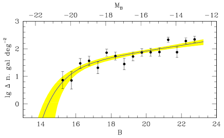
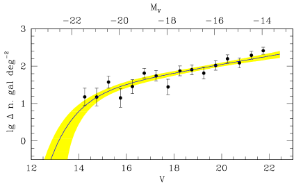
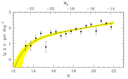
Figure 6: $B$, $V$ and $R$ band LF of red galaxies in Abell 1185. Data points and error bars are derived by binning the data in magnitude bins (and using an approximate error computation), whereas the curve traces the best fit LF of unbinned data and the shaded area marks the model uncertainty.

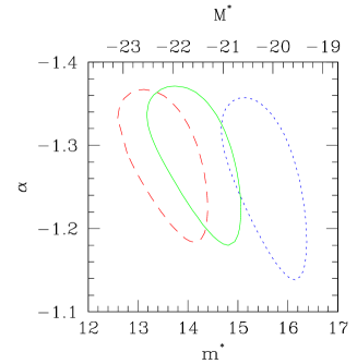
Figure 7: $B$, $V$ and $R$ (from right to left) 68 % confidence contours ($2\Delta\ln\mathcal{L}=2.30$) on $m^{*}$ ($M^{*}$ in the top x-axis) and $\alpha$.

3.2 The Luminosity function

3.2.1 Methods

Two methods are used to perform the statistical subtraction. For display purposes, we use the traditional method, put forward by, say, Zwicky (1957) and Oemler (1974) and summarized in many recent papers. The cluster luminosity function is computed as the difference between galaxy counts in the cluster and the control field directions, after binning the events (galaxy magnitudes) in magnitude bins. Approximate errors are computed as the square root of the variance of the minuend, because the contribution due to the uncertainty on the true value of background counts is negligible. Secondly, we fit the unbinned galaxy counts without any use of binned data or errors computed in the previous approach. At this point we follow the rigorous method set forth in APG, which is an extension of the Sandage, Tammann & Yahil method (1979, STY) to the case where a background population is present. The custom method adopts the extended likelihood instead of the conditional likelihood used by STY. The method (fully described in AGP) consists in fitting the unbinned distribution of clusters and control field counts using the likelihood, and in computing confidence intervals using the likelihood ratio theorem (Wilks 1938, 1963). The advantage of the rigorous method is that it provides unbiased results, reliable errors estimations, hence assuring the correctness of the result.

3.2.2 The LF of red galaxies

Fig 6 shows the resulting LFs of red galaxies in the three filters: the binned data with approximated error bars, and the best fit Schechter (1976) function with its uncertainty. Bins with incomplete data coverage are not plotted. The best fit parameters and their errors are listed in Table 1. This table also provides the range adopted for the fitting, a range such that the LF is unaffected by the $R<22.00$ mag initial selection.

68 % confidence contours are shown in Fig 7.

$m^{*}$ (or $M^{*}$) values, once values at the same slope $\alpha$ are considered, differ by the colour of red sequence galaxies (see Figure 7). $\alpha$ values in different bands are almost identical. This is expected, because no passband dependency of the red galaxies LF is possible as long as the colour-magnitude relation is linear. In fact, a linear mapping ($R$ to $B$ or $V$, in order to account for the colour-magnitude relation) has a constant Jacobian and cannot alter the shape of a distribution function. The detection of a passband dependency for a sample selected to obey to a linear colour–magnitude relation is instead a sign of problems in the data analysis.

The slope of the LF is determined with good accuracy ($\pm 0.06$) in all three bands but the uncertainty on the characteristic magnitude is large ($\approx 0.6$ mag), because we are studying a single not so rich cluster. We find that there are only about 20 red galaxies between $m_{3}$ and $m_{3}+2$ inside the studied portion of Abell 1185.

The best fit parameters are robust to the adopted width of the colour selection. Using a $\pm 0.2$ mag width in place of our reference $\pm 0.1$ mag width, we find in $R$: $m^{*}=13.9\pm 0.5$ and $\alpha=-1.18\pm 0.09$, in good agreement with the best fit parameters found by adopting a more stringent colour cut. Furthermore, 16 out of the 18 data points computed with the two colour selections differ each other by less than half the error bar in a non systematic way, clarifying that our reference colour boundary does not bias the LF. In particular, the above comparison shows that the Eddington bias is negligible, as expected.

Table 1: Fit results

filter	range	$m^{*}$	$\alpha$
$B$	$B<23.25$	$15.7\pm 0.5$	$-1.25\pm 0.06$
$V$	$V<22.45$	$14.3\pm 0.5$	$-1.28\pm 0.06$
$R$	$R<22.00$	$13.7\pm 0.7$	$-1.28\pm 0.06$

4 Comparison & Discussion

4.1 Comparison with the red sequences from other clusters

The red sequence of Abell 1185 has none of the specific features that are attributed to other clusters/environments by other works. The red sequence is linear and does not bend toward the blue at faint magnitudes, as Conselice et al. (2002) found for candidate members of the Perseus cluster. It neither bends toward the red as Evans et al. (1990) found for Fornax galaxies. The small scatter at faint magnitudes is much smaller than the half magnitude scatter that Conselice et al. (2002) found for candidate members of the Perseus cluster. Simply put in a few words, extremely faint galaxies in Abell 1185 follow the extrapolation of brighter red galaxies.

We underline that each of these features we do not detect may be reproduced by mismatches between cluster and control field images or by an incorrect estimation of the galaxy membership. On the other hand it is highly unlikely that these effects would render linear an intrinsically bended red sequence, or would strongly reduce the scatter of a scattered red sequence.

Our claim of a linear colour-magnitude of Abell 1158 is in apparent disagreement with the Ferrarese et al. (2006) claim of a non-linear colour–magnitude in Virgo. In order to cross check their results, we take advantage of the fact that the authors generously shared their data. We consider two models: a linear and a quadratic colour–magnitude relation, as considered by the authors. We assume normal errors on colours and an intrinsic scatter, and we compute the likelihood following the laws of probability (the likelihood for this problem is presented in D’Agostini 2005 and in the appendix of Andreon 2006). Computation of evidence (e.g. Liddle et al. 2004, for an astronomical introduction) and information content (e.g. Trotta 2005) clarify that either data are non-informative or, if any, they support the simpler model (a linear CM), and surely do not support the extended model (i.e. the quadratic CM). We note that while Ferrarese et al. (2006) acknowledge the existence of an intrinsic scatter, they do not account for it in the error computation (while it is accounted for in the present statistical analysis). Ignoring this component makes their fit to the bright and faint halves of their sample incompatible to each other, while they become compatible once the intrinsic scatter is accounted for.

Our approach, instead, is informative because it differentiates between a linear and non-linear model. Furthermore, we do not need any complex statistical analysis to differentiate them because of our small errors. Any potential 0.05 mag CM drift away from the linear CM is equal to the total observed scatter (intrinsic plus photometric scatter) around the CM in Abell 1185. For Virgo, it is one third of the observed scatter. In case of Abell 1185, a 0.1 mag drift is easily spotted even by eye (for example in Figure 3), whereas in case of Virgo it requires an advanced statistical analysis that ought to conclude that the data are largely un-informative about the colour-magnitude curvature.

We emphasize that there is no colour selection in Figure 3, and therefore we do not miss the possible CM bending (curvature) because of selection effects. A 0.05 mag drift away from a linear CM would lead to a distribution having different centers in the two panels by 0.05 mag, which is ruled out. In Figure 4, the colour selection ($\pm 0.2$ mag) is wider than a possible 0.05 mag drift and the CM does not become linear because its bending part is cut away by the colour selection.

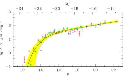
Figure 8: $V$ band LF of red galaxies in Abell 1185 (shaded region), Coma (Secker & Harris 1996; blue crosses), two $z=0.2$ clusters (Smail et al. 1998; green points), and nearby clusters in Tanaka et al. (2004; red triangles). All LFs are normalized (vertically shifted) to Abell 1185 down to $M_{V}=18$ mag. All LFs, but Tanaka et al. (2005), agree with each other. Abell 1185 goes deeper than the other LFs and has smaller errors.

4.2 Comparison with literature red galaxies LF

Figure 8 shows our $V$-band LF and its uncertainty (shaded region) and some literature red galaxies LFs. All LFs have been normalized to the richness (computed for galaxies brighter than $M_{V}=-18$ mag) of Abell 1185. Secker & Harris (1996) compute the LF of the Coma cluster in the $R$ band, converted to $V$ using the observed $V-R$ colour of Abell 1185 red galaxies. Smail et al. (1998) compute the $I$ band LF of red galaxies in some clusters at $z\sim 0.25$, well matching $V$-band observations in the cluster frame. In order to plot their data on Fig 8, we only need to compute the (small, 0.1 mag) E+K correction, derived using Bruzual & Charlot (2003), and the distance modulus of the studied clusters. These authors provide two red LFs, one based on the use of an homogeneous cluster and control field, plotted in Figure 8, and a second one using heterogeneous data (which is not considered here for the present comparison, in light of the mentioned difficulties in using heterogeneous data for LF studies). The red galaxy LF of Abell 1185 matches well these red galaxy LFs. Of course, every work adopts a slightly different definition of ’red galaxy’, such as a using a different width around the colour–magnitude (e.g. Secker & Harris 1996 choice is twice larger than ours), or increasing it with magnitude to account for a larger photometric scatter at fainter magnitudes (e.g. Smail et al. 1998), or using different filters (in both the observer and cluster frames). The current agreement of these LFs shows that the LF is robust to details in the ’red galaxy’ definition.

Figure 8 also shows the Tanaka et al. (2005) LF, computed in V band like our LF. It is $\approx 0.75$ mag too bright, for reasons that we are unable to understand.

Overall, our LF is in agreement with previous works. It is deeper and has smaller errors than previously published LFs, and thanks to the rigorous analysis, it is considered more reliable.

4.3 A more complex red galaxies LF?

In this section we ask ourself if our LF model should be updated in regards of published LFs, i.e. if the red galaxy LF is cluster-dependent; in particular whether we should use a more complex LF in order to account for the possible existence of a dip, i.e. a region with depressed counts, a feature actively debated in the literature (e.g. Biviano et al. 1995; Secker & Harris 1996).

We found no evidence for a dip in Abell 1185 (see Figure 6) and therefore we looked with further attention to the published claims about its existence. We consider with special attention Secker & Harris (1996), because the authors excel in accounting for the uncertainty in the background subtraction and in providing all the statistical details needed to re-analyse their data. They find that the LF of red galaxies in the Coma cluster is well modelled by a sum of a Gaussian and a Schechter, suggested by the presence of a possible dip in the Coma LF at $M_{R}\sim-19$ mag.

The simple Schechter model that best fit Abell 1185 data is a good description of their data (of Coma), being the $\chi^{2}=22$ for $15$ degree of freedom (i.e. larger $\chi^{2}$ are observed 10 % of the times under the null hypothesis that the data are drawn from the model), as can also qualitatively be seen in Fig 8. This comparison suggests that, in light of our results on Abell 1185 (which were of course not available at the time of their analysis) their data does not require a model more complex than a Schechter with $\alpha$ and $M^{*}$ fixed to the best fit Abell 1185 values. The Bayesian Information Criteria (Schwartz 1978; Lindle 2004 provides a useful astronomical introduction) quantitatively informs us that evidence is largely in favor of the simplest model.

We cannot repeat the above analysis to other published works because they usually do not provide all the necessary details. Qualitatively, a model with a dip seems unnecessary, even when the $p$ value of the data (computed using the $\chi^{2}$ or another statistic) is small (i.e. the fit with a Schecther function is claimed to be bad), since the increase in log-likelihood obtained by introducing the extra parameters is more than compensated by the huge increase in dimensionality of the parameter space over which likelihood should be averaged.

4.4 Discussion on methods

4.4.1 Impact of the method used

Compared to previously published works, the CM presented in this study has been determined in a fairly different way, and therefore it is important to discuss whether our results may depend or not on the analysis method. We derived all our results twice: first using the common method currently used in literature, and then using a statistical method based on axioms of probabilities. The two methods give the same results qualitatively but the second method has the advantage of providing results with guaranteed correctness, at the difference of a blind application of basic rules potentially giving misleading results, as detailed also in APG, Andreon et al. (2006), and also by several previous works (e.g. Kraft et al. 1991; Loredo 1992).

The most notable difference between our study and the previous works is that instead of subtracting the background of galaxies, we account for it more rigorously. The present work is a continuation of activities started in APG, and continued in Andreon et al. (2006) and Andreon (2006).

The usual astronomical recipe for background subtraction, $n_{clus}=n_{tot}-n_{bkg}$, called unbiased estimator by sampling theories (e.g. MacKay 2005), has a somewhat different meaning from what it seems. Let us suppose, for example, that 3 galaxies are observed in the cluster line of sight, and 5 are expected given our (assumed to be quite precise) control field observations. This situation is possible, because of Poisson fluctuations. If we compute the cluster contribution as the difference between the above two numbers, we find a negative number of galaxies in the cluster (or say in a given location of the parameter space, i.e. in a given range of colours and mag), leading to the unphysical result of non-positive numbers of galaxies. Therefore, $n_{tot}-n_{bkg}$ is an estimator of $n_{clus}$ that in certain conditions has properties that are not acceptable.

A naive solution to avoid unphysical values is to set these negative values to zero. However, this correction overestimates the total number of cluster galaxies (i.e. the one of the whole sample), because negative fluctuations have been corrected all in the same direction by increasing them, and positive fluctuations left untouched (effectively a Malmquist-type bias). Another possible naive solution is to widen the bin size (if data are binned), until unphysical values disappear. Physically, it may happen that the bin becomes much larger in a direction than the uncertainty of the data points it contain. In such a situation, in order to remove an unphysical result we are forced first to put in the same bin incompatible data (because at several $\sigma$’s away from each other), and then to subtract off each other incompatible data, a procedure which can only lead to doubtful results. This situation often occurs at the less populated bright magnitudes, where errors are small.

Therefore, if $n_{tot}-n_{bkg}<0$, we are in an unsatisfactory position: we may choose between: a) having unphysical values at some location and an unbiased total number count, or b) having physical values for individual measurements and a biased value for the whole sample, or c) adding/subtracting each other incompatible data points. Actually, the same problem holds for $n_{tot}-n_{bkg}\ga 0$ (of which some aspects are called Malmquist bias in literature, see Jeffreys 1938 for a lucid discussion), and has already been discussed in Kraft et al. (1991), APG and Andreon et al. (2006) and others. As soon as the dimensionality of the data space is large, or when, as in the present case, the distribution of the data in the data space is uneven, there will always been some bins/location where $n_{tot}-n_{bkg}\approx 0$, i.e where some problems arise.

The second shortcoming of the usual astronomical recipe, $n_{tot}-n_{bkg}$, concerns the measurement of its uncertainty. When the difference above is negative, a confidence interval (at whatever confidence level) is an empty interval (Kraft et al. 1991). With the confidence interval empty, no interval can be shorter, not even the one derived in absence of any background, an incoherent result. For example, contrary to common sense, one may conclude because of that approach that it makes no sense to perform a redshift survey to determine the individual membership of every galaxy in the sample, because these new observations will lead to larger confidence intervals! The null length of the confidence interval produces another absurd result: let us suppose that the derived confidence interval turns out to be of positive length. There is an easy way to make it smaller: by adding a background in the hope that Poisson fluctuations make $n_{tot}-n_{bkg}<0$. For a sufficiently large background the above occurs 50 % of the times. Such a solution, although formally correct, is unacceptable intuitively since it implies adding noise in order to reduce uncertainties!

The third shortcoming of the usual astronomical recipe comes from binning the data. As discussed in APG, seldom the size, number and location of bins are considered, as well as their relevance for the final results. Does a trend has been missed because the non-optimal quantization of data in bins?

Bayesian methods do not present such troubles, because: a) they do not require that data are binned; b) they are squarely based on axioms of probabilities (i.e. returning credible intervals in agreement with logic and common sense). [START NEW TEXT] Specifically, instead of removing the background, we introduced the background component, and we then marginalize the posterior over the nuisance (background) parameters, as required by the sum axiom of probability. [END NEW TEXT] c) they naturally account for boundaries in the data or parameter space. In the present work several parameters have boundaries: for example, the intrinsic scatter of the colour-magnitude relation and the number of cluster or field galaxies cannot be negative.

Therefore, for display purposes we use astronomical recipes, which often hold, but adopted a full Bayesian computation for estimating parameters (and uncertainties) and for model selection. Appendix of Andreon (2006) describes in detail the stochastical computation using the Monte Carlo Marcov Chain (MCMC, Metropolis 1953) method used to determine the colour–magnitude relation.

The full Bayesian computation and the use of common rules, both provide compatible results: in fact, in all figures showing data points computed with astronomical recipes, and models computed with probability axioms, the two derivations agree each other. For example, curves and data points in Figure 6 agree with each other. The colour–magnitude slope derived from theory of probabilities (solid line in Figure 2) agrees data points in Figure 2. The full Bayesian computation is however not useless. The agreement between the two approaches has been “guided” by the more precise computation: for example, in Figure 6 by taking much smaller bins, we easily get negative numbers of cluster galaxies and also an unbelievable luminosity function that takes only discrete values (because cluster galaxies come in integer units), an unphysical result. Furthermore, “guided” by the Bayesian analysis in Figure 6 we did not plot confidence intervals (that have the mentioned shortcoming of not becoming small when the uncertainty on nuisance parameters decreases and of potentially being of null lenght), but we computed the (approximated) variance of the estimator $n_{tot}-n_{bkg}$. One of the advantages of Bayesian methods is that they always return numbers with guaranteed correctness, the disadvantage is that sometime they are expensive to implement computationally.

The LF is determined strictly following APG, i.e. a maximum likelihood method, to which we defer for details, instead of a determination from a fully Bayesian derivation. In the present paper, we took advantage from the fact that regularity conditions for the use of the likelihood ratio theorem holds for LF computations, and therefore we used the inexpensive maximum likelihood method instead of cpu–expensive Bayesian approach for the stochastical computations.

4.4.2 The role of assumptions

During our CM determination in the Appendix, we made several assumptions. First of all, we determined the slope of the colour–magnitude assuming its linearity. However if the colour–magnitude is bended, the meaning of “slope” (a number, indeed) is ill defined: what is the slope of a bended line? Therefore, a valid question that precedes the slope determination is: does the colour–magnitude is bended or linear? This task is named model selection, and we met it when discussing this very same issue for Virgo galaxies (sec 4.1), and again when we commented about the existence of a dip in the LF (sec 4.2). As done in sec 4.1, to answer the question, it is just matter of increasing the degree of the polynomial describing the colour–magnitude relation shape and compare the relative evidence of the two models: the linear model turns out to be highly preferred. The outcome of this comparison is quite expected, the colour–magnitude is clearly linear, as the inspection of Figure 4 at bright magnitudes clearly demonstrate, as well as Figure 3 at faint magnitudes, and Figure 5 over the whole magnitude range. The first two plots are two simple projections of the data cube, no analysis whatsoever has been applied. In Figure 5, instead, the background has been removed, by quantizing data in bins in the colour–colour–magnitude plane.

Second, we further assumed that the LF of red galaxies is described by a Schechter function and that the distribution of background galaxies can be modelled as a polynomial in the restricted range of colours we are interested in. The former assumption is justified by Figure 6 (see the data points, derived without any assumption about the LF shape). The latter assumption is quite general: every distribution sufficiently smooth can be approximated by its Taylor expansion, which is a polynomial. Therefore, we raised the degree of the polynomial until a satisfactory match with the data is reached.

4.4.3 Conclusions on methods

The performed analysis squarely relies on laws of probabilities and accounts for the existence of boundaries. It is possible to follow a simpler path to derive the results, of course, but we cannot guarantee the correctness of the results obtained by methods that ignore (or not fully account for) laws of probabilities and ignore the existence of boundaries in the data or parameter space.

4.5 Discussion on results

The colour-magnitude relation has a simple interpretation in the context of galaxy formation: the brighter and more massive galaxies have deeper gravitational potential wells, and therefore are more prone at retaining the interstellar gas which becomes superheated and metal enriched during initial stages of the star-formation epoch (Dekel & Silk 1986). Assuming that the magnitude blueing of the red sequence is only due to metallicity, and adopting the Harris (1996) [Fe/H] vs $B-R$ calibration, galaxy metallicity changes by 1.2 dex in the explored magnitude range. Although the colour-magnitude sequence is interpreted in terms of a metallicity trend (Kodama & Arimoto 1997), our data alone may be interpreted in terms of age (fainter galaxies are younger and thus bluer), because of the well known age/metallicity degeneracy (e.g. Worthey 1994).

Abell 1185 does not present the appealing features claimed to have been observed in other clusters and discussed at length in previous published works. Its red sequence does not disappear at faint magnitudes, neither bends toward red or blue colours: it simply continues straight, following the extrapolation of what is usually observed at brighter magnitudes. The scatter along the CM does not largely increase with magnitude as claimed for galaxies in the Perseus clusters. The LF of red galaxies shows no dip and no pass-band dependency.

All the above points offer us the chance of not looking for physical mechanisms affecting the objects features in such a way to produce the (unobserved) heterogeneity. The absence of features points toward an homogeneity of red galaxies over the whole nine magnitude range explored (four decades in stellar mass). Our argument is the usual one, and can be found on most papers discussing the homogeneity of red galaxies (e.g. Bower, Lucey & Ellis 1992; Andreon 2003), with the only difference that what is discussed for bright galaxies holds here for the extreme faint galaxies: homogeneity in colour implies an old star age or a synchronization between the history of star formation of the various galaxies.

Faint ($M\approx M^{*}+3$ mag) red galaxies have attracted the attention of astronomers in recent days. At high redshift the colour magnitude relation sees signs of depletions, i.e. it has been reported that at $M^{*}+2.5$ the colour-magnitude relation disappears (Kodama et al. 2004) or it is strongly underpopulated (De Lucia et al 2004). On the other end, the effect does not appear to be universal, since the $z=0.83$ MS 1054 cluster does not show any signs of depletion (Andreon, 2006) down to $M^{*}+3.5$ mag. We defer to Andreon (2006) for a detailed discussion about the reality of the claimed deficit of faint red galaxies. Kodama et al. (2004) and De Lucia et al (2004) conclude that faint ($M^{*}+3$) red galaxies are a recent ($z\la 1$) population. This interpretation does not fit our data: if faint red galaxies are younger than brighter red galaxies, then they should not lay on the extrapolation at faint magnitude of the CM relation observed at brighter magnitudes (i.e. the CM should bend toward the blue) and the scatter should increase toward faint magnitudes (there is less time for the objects to make their colour more similar). Quantification of the offset to be observed is simple: if faint galaxies form at $z\sim 0.8$ instead of $z\sim 3$, they should be bluer by 0.06 mag in $B-V$ (assuming a single stellar population, e.g. Buzzoni 2005), a drift that we do not see in Abell 1185.

5 Conclusions

We have studied the colour of red galaxies of the Abell 1185 cluster at $z=0.0325$ down to $M^{*}+8$ in the $B$, $V$ and $R$ bands. The colour–magnitude relation is linear without evidence for a significant bending down to absolute magnitudes seldom probed in literature ($M_{R}=-12.5$ mag). It is also thin ($\pm 0.04$ mag) and its thickness is not a strong function of magnitude. The luminosity function of red galaxies in Abell 1185 is adequately described by a Schechter function, with characteristic magnitude and faint end slope that also well describe the LF of red galaxies in other clusters. There is no passband dependency of the LF shape, other than an obvious $M^{*}$ shift due to the colour of the considered population. Red galaxies form an homogeneous population, over four decades in stellar mass, for what concerns colours and luminosity. Homogeneity in colour implies an old star age or a synchronization between the history of star formation of the various galaxies, down to $M^{*}+8$.

Appendix A Thecnical details

In section 3 we do not provide quantitative details about the way the slope and scatter of the colour–magnitude relation of cluster galaxies have been determined, a gap that we fill in this appendix. We strictly follow Andreon (2006) who presents the statistical approach, starting from axioms of probability and largely following D’Agostini (2003; 2005). In short, we model the cluster distribution in the colour–magnitude plane as the product of a Schechter function in mag and a linear colour–magnitude relation with an intrinsic unknown scatter. Furthermore, we model the background distribution in the colour–magnitude plane as the product of a power law of degree two in mag and of degree one in colour times a Gaussian in colour with unknown dispersion whose central colour is linear depending on mag with unknown slope and intercept. Such a modeling requires seven nuisance parameters for the background, over which we marginalize in order to derive the uncertainty on the interesting quantities (e.g. the parameters describing the colour-magnitude relation). The wide magnitude range and the aboundant background data considered in this paper, both oblige us to adopt a model with many parameters for the background and such a complicate model is still insufficient to describe the background distribution over the whole magnitude range accessible to the observations. Instead than increasing the model complexity of the background (which encodes information which is not of our interest in this paper), we prefers to discard the last magnitude bin where the background contribution is so large than they carry a very poor information about the slope and intercept of the colour–magnitude relation (i.e. in our CM determination we use $R<21$ instead of $R<22$). One of the merit of this approach is not to claim plausible that the CM has a negative scatter, feature that instead blesses other methods that claim that negative (and therefore unphysical) values of the scatter are within the 68 % confidence interval.

As in Andreon (2006), we are not interested in modelling the distribution of red galaxies at colours where they are not observed and therefore we limit the analysis to the $0.4<V-R<0.9$ mag and $0.7<B-V<1.5$ mag ranges. Assuming uniform priors zero-ed in the unphysical ranges, we found:

$B-V=0.986\pm 0.007-(0.038\pm 0.003)(R-19.556)$ mag with a scatter of 0.039 mag and

$V-R=0.608\pm 0.007-(0.016\pm 0.002)(R-19.556)$ mag with a scatter of 0.036 mag.

References

- Abell (1958) Abell, G. O. 1958, ApJS, 3, 211
- Andreon (2003) Andreon, S. 2003, A&A, 409, 37
- Andreon (2006) Andreon, S. 2006, MNRAS, 369, 969
- Andreon & Cuillandre (2002) Andreon, S., & Cuillandre, J.-C. 2002, ApJ, 569, 144
- Andreon et al. (2004) Andreon, S., Lobo, C., & Iovino, A. 2004, MNRAS, 349, 889
- Andreon et al. (2005) Andreon, S., Punzi, G., & Grado, A. 2005, MNRAS, 360, 727
- Andreon et al. (2006) Andreon, S., Quintana, H., Tajer, M., Galaz, G., & Surdej, J. 2006, MNRAS, 365, 915
- Baldry et al. (2004) Baldry, I. K., Glazebrook, K., Brinkmann, J., Ivezić, Ž., Lupton, R. H., Nichol, R. C., & Szalay, A. S. 2004, ApJ, 600, 681
- Bertin & Arnouts (1996) Bertin, E. & Arnouts, S. 1996, A&AS, 117, 393
- Biviano et al. (1995) Biviano, A., Durret, F., Gerbal, D., Le Fevre, O., Lobo, C., Mazure, A., & Slezak, E. 1995, A&A, 297, 610
- Blanton et al. (2005) Blanton, M. R., Lupton, R. H., Schlegel, D. J., Strauss, M. A., Brinkmann, J., Fukugita, M., & Loveday, J. 2005, ApJ, 631, 208
- Bower et al. (1992) Bower, R. G., Lucey, J. R., & Ellis, R. S. 1992, MNRAS, 254, 601
- Bruzual A. & Charlot (1993) Bruzual A., G., & Charlot, S. 1993, ApJ, 405, 538
- Conselice et al. (2002) Conselice, C. J., Gallagher, J. S., & Wyse, R. F. G. 2002, AJ, 123, 2246
- Cuillandre et al. (2000) Cuillandre, J.-C., Luppino, G., Starr, B. & Isani, S., 2000, SPIE, 4008, 1010
- D’Agostini (2003) D’Agostini, G. 2003, ”Bayesian reasoning in data analysis - A critical introduction”, World Scientific Publishing
- D’Agostini (2005) D’Agostini, G. 2005, preprint, (physics/0511182)
- Dekel & Silk (1986) Dekel, A., & Silk, J. 1986, ApJ, 303, 39
- De Lucia et al. (2004) De Lucia, G., et al. 2004, ApJ, 610, L77
- Drinkwater et al. (1999) Drinkwater, M. J., Phillipps, S., Gregg, M. D., Parker, Q. A., Smith, R. M., Davies, J. I., Jones, J. B., & Sadler, E. M. 1999, ApJ, 511, L97
- Evans et al. (1990) Evans, R., Davies, J. I., & Phillipps, S. 1990, MNRAS, 245, 164
- Ferrarese et al. (2006) Ferrarese, L., et al. 2006, ApJS, in press (astro-ph/0602297)
- Garilli Maccagni & Andreon (1999) Garilli, B., Maccagni, D. & Andreon, S. 1999, A&A, 342, 408
- Jeffreys (1938) Jeffreys, H. 1938, MNRAS, 98, 190
- Jones & Forman (1984) Jones, C., & Forman, W. 1984, ApJ, 276, 38
- Harris (1996) Harris, W. E. 1996, AJ, 112, 1487
- Kodama et al. (2004) Kodama, T., et al. 2004, MNRAS, 350, 1005
- Kodama & Arimoto (1997) Kodama, T., & Arimoto, N. 1997, A&A, 320, 41
- Landolt (1992) Landolt, A. U. 1992, AJ, 104, 340
- Liddle (2004) Liddle, A. R. 2004, MNRAS, 351, L49
- (31) Loredo, T., 1992, in ”Statistical Challenges in Modern Astronomy”, eds. E. D. Feigelson and G. J. Babu (New York: Springer-Verlag) pag. 275
- (32) MacKay D., 2005, Information theory, Inference and Learning Algorithms, Cambridge University Press
- Magnier & Cuillandre (2004) Magnier, E. A., & Cuillandre, J.-C. 2004, PASP, 116, 449
- Mahdavi et al. (1996) Mahdavi, A., Geller, M. J., Fabricant, D. G., Kurtz, M. J., Postman, M., & McLean, B. 1996, AJ, 111, 64
- Mateo (1998) Mateo, M. L. 1998, ARA&A, 36, 435
- McCracken et al. (2003) McCracken, H. J., et al. 2003, A&A, 410, 17
- Oemler (1974) Oemler, A. J. 1974, ApJ, 194, 1
- Sandage, Tammann, & Yahil (1979) Sandage, A., Tammann, G. A., & Yahil, A. 1979, ApJ, 232, 352
- Secker et al. (1997) Secker, J., Harris, W. E., & Plummer, J. D. 1997, PASP, 109, 1377
- Secker & Harris (1996) Secker, J., & Harris, W. E. 1996, ApJ, 469, 623
- Schechter (1976) Schechter, P. 1976, ApJ, 203, 297
- (42) Schwarz G., 1978, Annals of Statistics, 5, 461
- Smail et al. (1998) Smail, I., Edge, A. C., Ellis, R. S., & Blandford, R. D. 1998, MNRAS, 293, 124
- Tanaka et al. (2005) Tanaka, M., Kodama, T., Arimoto, N., Okamura, S., Umetsu, K., Shimasaku, K., Tanaka, I., & Yamada, T. 2005, MNRAS, 362, 268
- Trotta (2005) Trotta, R. 2005, preprint, (astro-ph/0504022)
- Visvanathan & Sandage (1977) Visvanathan, N., & Sandage, A. 1977, ApJ, 216, 214
- (47) Wilks, S., 1938, Ann. Math. Stat. 9, 60
- (48) Wilks, S., 1963, Mathematical Statistics (Princeton: Princeton University Press).
- Worthey (1994) Worthey, G. 1994, ApJS, 95, 107
- Zwicky (1957) Zwicky, F. 1957, Morphological Astronomy, Berlin: Springer