Constraining Isocurvature Initial Conditions with WMAP 3-year data

Abstract

We present constraints on the presence of isocurvature modes from the temperature and polarization CMB spectrum data from the WMAP satellite alone, and in combination with other datasets including SDSS galaxy survey and SNLS supernovae. We find that the inclusion of polarization data allows the WMAP data alone, as well as in combination with complementary observations, to place improved limits on the contribution of CDM and neutrino density isocurvature components individually. With general correlations, the upper limits on these sub-dominant isocurvature components are reduced to $\sim$60% of the first year WMAP results, with specific limits depending on the type of fluctuations. If multiple isocurvature components are allowed, however, we find that the data still allow a majority of the initial power to come from isocurvature modes. As well as providing general constraints we also consider their interpretation in light of specific theoretical models like the curvaton and double inflation.

I Introduction

Impressive recent developments in measurements of the Cosmic Microwave Background (CMB) temperature and polarization anisotropies Hinshaw:2006ia ; Jarosik:2006ib ; Page:2006hz ; Spergel:2006hy , large scale structure (LSS) 2df ; Tegmark:2003uf ; Seljak:2004sj ; Eisenstein:2005su ; Cole:2005sx , supernovae Riess:2004nr ; Astier:2005qq and the Lyman-$\alpha$ forest Seljak:2006 have enabled stringent testing of the cosmological model including the composition of the universe and the initial conditions that seeded inhomogeneities. Although the simplest initial conditions, arising from single field inflation, predict scale-invariant, adiabatic inhomogeneities, this is far from the only possibility. Isocurvature modes are predicted by a wide range of scenarios, for example multi-field inflation Polarski:1994rz ; Garcia-Bellido:1995qq ; Linde:1996gt ; Pierpaoli:1999zj ; Kawasaki:2001in , topological defects Battye:1998xe ; Battye:1999em , and through the decay of particles prior to nucleosynthesis such as a scalar curvaton Lyth:2001nq ; Moroi:2001ct ; Bartolo:2002vf ; Moroi:2002rd ; Lyth:2002my ; Dimopoulos:2003ii ; Dimopoulos:2003az , axions Bozza:2002fp or the Affleck-Dine model of baryogenesis Kawasaki:2001in . The degree of correlation with adiabatic perturbations can vary across the full spectrum, from completely (anti) correlated in the curvaton scenario, intermediate correlation in some multi-field inflation models, to uncorrelated modes in cosmic string scenarios. Most proposed scenarios generate solely baryon or Cold Dark Matter (CDM) isocurvature modes cdm_theory ; mechanisms generating neutrino density and velocity isocurvature modes are also possible nu_theory ; BMT:2000 , though the latter are more difficult to motivate.

Although the simplest adiabatic scenario is in complete agreement with the current data Spergel:2006hy , the question still arises, how large a contribution could isocurvature modes make and how sensitive is the cosmological parameter estimation to their inclusion? In this paper we confront these questions, specifically focusing on constraints from the WMAP CMB temperature and polarization power spectra Jarosik:2006ib ; Hinshaw:2006ia ; Page:2006hz ; Spergel:2006hy , SDSS galaxy matter power spectrum Tegmark:2003uf and the SNLS supernovae survey Astier:2005qq . Experiments in the past ten years have ruled out models with purely isocurvature perturbations Stompor:1995py ; Langlois:2000ar ; Enqvist:2000hp ; Amendola:2001ni , but have not excluded those with admixtures of adiabatic and isocurvature modes. Constraints placed on models with a single isocurvature mode, in light of the first year WMAP results, indicate that it must be sub-dominant Peiris:2003ff ; Valiviita:2003ty ; crotty:03 ; Gordon:2003hw ; beltran:04 ; Moodley:2004nz ; Kurki-Suonio:2004mn ; Beltran:2005gr , but models with multiple modes may have larger non-adiabatic contributions Bucher:2004an ; Moodley:2004nz ; Dunkley:2005va . Here we analyze the constraints in light of the 3-year WMAP data release of temperature and polarization data for which only an analysis for perfectly correlated CDM or baryon isocurvature perturbations has been conducted so far Lewis:2006ma ; Seljak:2006 .

In section II we outline the approach and parameterizations used in the analysis. In sections III and IV we respectively establish the constraints on scenarios with purely correlated and generally correlated single isocurvature modes. In doing so we reflect on what the limits on isocurvature contributions imply for some key particle based theories which depart from purely adiabatic perturbations. In section V we expand our analysis to allow multiple isocurvature modes with general correlations, in which destructive cancellations can allow a large fractional isocurvature contribution. We conclude with a summary of our findings and implications for future cosmological observations in section VI.

II Approach

Perturbations to the metric may give rise to both curvature perturbations on comoving hypersurfaces, as well as entropy perturbations where the space-time curvature vanishes at early times. The former are termed adiabatic perturbations and may be quantified by the curvature perturbation, $\cal R$. The latter are isocurvature modes, quantified by the entropy perturbation ${\cal S}_{x}=\delta\rho_{x}/(\rho_{x}+p_{x})-\delta\rho_{\gamma}/(\rho_{\gamma}+p_{\gamma})$ in the case of density perturbations, $\delta\rho$, between photons and a fluid $x$, which may be CDM or baryons. There are two further isocurvature modes where the sum of the neutrino and photon densities, or momentum densities, are initially unperturbed, whose initial conditions are given in BMT:2000 ; camb .

To first order, initial conditions $\delta\rho_{c}=-\delta\rho_{b}$, $\delta\rho_{\gamma}=\delta\rho_{\nu}=0$ allow a time independent solution to the perturbation equations for the pressureless matter components. Baryon and CDM isocurvature initial conditions, up to a factor of $\Omega_{c}/\Omega_{b}$, are essentially observationally indistinguishable and therefore we only consider CDM isocurvature scenarios of the two here.

The perturbations may be characterized using the covariance matrix $\Delta$, where

$$\Delta_{ij}(k)\delta^{3}({\bf k}-{\bf k^{\prime}})=\left(\frac{k}{2\pi}\right)^{3}\langle{\chi}_{i}({\bf k})\,{\chi}_{j}^{*}({\bf k^{\prime}})\rangle$$ (1)

as shown in BMT:2000 . The subscript $i$ may take the values {A,C,N,V}, labeling the adiabatic (AD), CDM isocurvature (CI), neutrino isocurvature density (NID), and neutrino isocurvature velocity (NIV) components respectively, and the random variable $\chi_{i}$ corresponds to the amplitude of the $i$th mode.

We assume that the elements of the matrix $\Delta$ can be parameterized as

$$\Delta_{ij}(k)={\cal A}_{ij}~{}\left(\frac{k}{k_{0}}\right)^{n_{ij}-1},\qquad n_{ij}={1\over 2}(n_{i}+n_{j})$$ (2)

in terms of a set of amplitude parameters ${\cal A}_{ij}$, power-law spectral indices $n_{i}$, and the pivot value $k_{0}=0.05$ /Mpc.

The angular power spectrum of a given correlation $ij$ is given by

$$C_{\ell}^{ij}=\int_{0}^{\infty}\frac{dk}{k}\Delta_{ij}^{2}(k)\Theta_{\ell}^{i}(k)\Theta_{\ell}^{j}(k),$$ (3)

where $\Theta_{\ell}^{i}(k)$ is the photon transfer function for initial condition $i$. An admixture of the adiabatic mode with a single isocurvature mode can be expressed in terms of the pure adiabatic, isocurvature and wholly correlated spectra, such that

$$C_{\ell} = {\cal A}_{AA}C_{\ell}^{AA}+{\cal A}_{II}C_{\ell}^{II}+2{\cal A}_{AI}C_{\ell}^{AI},$$ (4)

where $I$ labels $C,N$ or $V$. This is commonly parameterized using one of the following:

$$C_{\ell} = C_{\ell}^{AA}+B^{2}C_{\ell}^{II}+2B\cos\theta C_{\ell}^{AI},$$ (5)

$$= (1-\alpha)C_{\ell}^{AA}+\alpha C_{\ell}^{II}+2\beta\sqrt{\alpha(1-\alpha)}C_{\ell}^{AI},$$ (6)

to within an overall normalization factor, with the former used by Amendola:2001ni ; Valiviita:2003ty ; Peiris:2003ff and the latter by crotty:03 ; beltran:04 ; Beltran:2005gr . Using equation (6), the amplitude and correlation phase of the isocurvature contribution are given by $\alpha$ and $\beta$ respectively. These in turn can be related to the overall ratio of isocurvature to adiabatic component given by $B={\cal S}/{\cal R}$, with $\alpha=B^{2}/(1+B^{2})$, and general correlation $\beta=\cos\theta$. We will use $\alpha$ and $\beta$ as parameters in this analysis, for models with a single isocurvature mode, sampling with $\beta$ directly rather than $2\beta\sqrt{\alpha(1-\alpha)}$. With these definitions, a positive correlation between the adiabatic and isocurvature perturbations will produce a wholly correlated CMB spectrum with a negative amplitude at large scales, in agreement with e.g. Amendola:2001ni ; Peiris:2003ff ; Valiviita:2003ty ; beltran:04 and the CAMB package. The primordial adiabatic perturbation may be defined such that these correlated spectra have the opposite sign, as used in Bucher:2004an ; Moodley:2004nz ; Kurki-Suonio:2004mn ; Dunkley:2005va .

The above parameterizations do not naturally extend to the addition of more than one isocurvature mode, for which a method is given in Bucher:2004an ; Moodley:2004nz . Here

$$C_{\ell}=\sum_{ij=1}^{N}{z_{ij}}\hat{C}_{\ell}^{ij}$$ (7)

for $N$ perturbation modes, where $\sum_{i,j=1}^{N}z_{ij}^{2}=1$, and any matrix $z$ with a negative eigenvalue is assigned a zero prior probability. $\hat{C}_{\ell}$ are normalized to have equal CMB power in each mode $i$, such that $z_{ij}$ quantify the physically observable power in each mode¹ . By definition the coordinates $z_{ij}$ lie on the surface of a $N^{2}$-dimensional unit sphere, which can be sampled uniformly with $N^{2}-1$ amplitude parameters using the volume preserving mapping shown in Moodley:2004nz . To quantify the isocurvature contribution in the case of multiple modes, a measure is given by $r_{iso}={z_{iso}}/{(z_{iso}+z_{AA})}$, where $z_{iso}=\sqrt{1-z_{AA}^{2}}$. This is equivalent to the $f_{iso}$ parameter in Bucher:2004an ; Moodley:2004nz ; Dunkley:2005va , but different to the $f_{iso}$ used in e.g. Peiris:2003ff ; Valiviita:2003ty ; Beltran:2005gr , which corresponds to $B$ in equation  (6).

It is important to note that constraints on $\alpha$ can depend strongly on the pivot scale, whereas the ${z_{ij}}$ parameters are independent of the pivot. As such, the $z_{ij}$ parameterization is a useful direct measure of isocurvature, whereas $\alpha$ can be misleading when the isocurvature and adiabatic spectral tilts are allowed to vary independently, as will be discussed in section IV. For ease of comparison with previous analyses, however, for single components we present constraints for $\{\alpha,\beta\}$ (pivoted at $k=0.05/$Mpc) and give equivalent constraints on $\{z_{ij}\}$, since the relation between the single mode parameterization $\{\alpha,\beta\}$ and the $\{z_{ij}\}$ is not trivial. For multiple modes we solely present results using the $\{z_{ij}\}$ parameterization.

We parameterize our cosmological model in terms of a $\Lambda$CDM scenario using the following parameters: $\Omega_{b}h^{2},\Omega_{c}h^{2},\tau,\Omega_{\Lambda},b_{SDSS}$, and an overall scalar amplitude parameter, limiting our search to flat models with scalar fluctuations and assume 3.04 massless neutrinos species with zero chemical potential. We do not investigate here broader parameter spaces including tensor modes, running in the scalar spectral index, spatial curvature or evolving dark energy. Throughout this paper we use a single parameter $n_{s}$ for both the isocurvature and adiabatic spectral index. However, we do relax this constraint in section IV where we discuss the implications of a single CDM isocurvature mode generally correlated with the adiabatic one.

We find constraints using the 3-year WMAP CMB data alone Hinshaw:2006ia ; Page:2006hz for CDM and neutrino density isocurvature scenarios with a variety of degrees of correlation, and constraints on one, two and three isocurvature components more generally in combination with data from the SDSS galaxy survey Tegmark:2003uf , including a Gaussian prior on the SDSS bias measurement $1.03\pm 0.15$ Seljak:2004sj and non-linear corrections halofit , and supernova data from SNLS Astier:2005qq . We include BBN estimates of the baryon to photon ratio, conservatively encompassing measurements of both Deuterium ($\eta_{10}=6.4\pm 0.7$) and Helium-3 ($\eta_{10}=6.0\pm 1.7$) Steigman:2005uz by imposing a Gaussian prior of $\Omega_{b}h^{2}=0.022\pm 0.006$. Small-scale polarization data do not yet noticeably tighten the constraints so we do not include them in the analysis. As we discuss in the analysis and conclusion, however, future small scale polarization data could well be an important test of isocurvature scenarios. We generate CMB and matter power spectra using the CAMB package camb , which is consistent with our perturbation definitions. The likelihood surfaces are explored using Markov Chain Monte Carlo methods, applying the spectral convergence test described in dunkley , and the Gelman and Rubin convergence test gelman . We also use a downhill simplex method to find the best-fit likelihood, starting from the maximum likelihood point sampled by the chains, since the likelihood peak is only sparsely sampled by MCMC in high dimensional spaces.

III Uncorrelated and perfectly correlated isocurvature: single modes

In a variety of theoretical scenarios the isocurvature and adiabatic fluctuations in matter can arise out of a single mechanism and subsequently have well-defined degrees of correlation. We first consider constraints on purely correlated ($\beta=1$), uncorrelated ($\beta=0)$ and anti-correlated ($\beta=-1$) CDM and neutrino density isocurvature fluctuations from WMAP data alone (TT+TE+EE), and in combination with other datasets. Figure 1 shows that for both CDM and neutrino density isocurvature, purely correlated scenarios are the most tightly constrained by the data. For CDM modes with WMAP+SDSS+SNLS+BBN (and WMAP only) we find $\alpha<0.009(<0.01)$ at 95% confidence limit (c.l.) for purely correlated and $<0.009(<0.045)$ for anti-correlated modes (consistent with Seljak:2006 , who find $\alpha<0.005$ including Ly-$\alpha$ data). The corresponding limits for neutrino density modes are $\alpha<0.017(<0.025)$ and $<0.026(<0.083)$. The wholly uncorrelated isocurvature modes are allowed to contribute a much more significant fraction of the overall power, with $\alpha<0.11(<0.26)$ and $\alpha<0.21(<0.55)$ (95% c.l.) for CDM and neutrino density isocurvature modes. We consider the statistical support for presence of isocurvature flucutations by using the bestfit likelihood , ${\cal L}$, calculated by comparing the theoretical spectrum predicted by the cosmological scenario, $\{C_{l}^{th}\}$, to the observed temperature and polarization maps or spectra, x, in light of the statistical and systematic errors encoded in the covariance matrix C,

$${\cal L}({\bf x}|C_{l}^{th})=\prod_{datasets}\frac{\exp[{\bf xC}^{-1}{\bf x}/2]}{\sqrt{\det C}}.$$ (8)

The 3-year WMAP data is entirely consistent with no isocurvature contribution being required, having no improvement over the bestfit likelihood for the adiabatic scenario $-2\ln{\cal L}$ = 11252 ( arising from the joint pixel/ spectrum based likelihood approach outlined in Hinshaw:2006ia ; Spergel:2006hy with total $\chi^{2}=\sum{\bf xC}^{-1}{\bf x}=3279$ for 3244 degrees of freedom and $\sum\ln\det C=7973$ ).

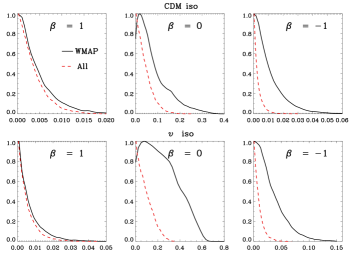
Figure 1: 1-dimensional likelihood distributions for CDM (top) and neutrino (bottom) density isocurvature models with perfectly correlated $\beta=1$, anti-correlated $\beta=-1$ and uncorrelated $\beta=0$ isocurvature perturbations using WMAP only data (black full) and combined with SDSS, SNLS and BBN data (red dashed).

For WMAP data alone significant cosmological parameter degeneracies exist between $\alpha$ and $\Omega_{c}h^{2}$ and $n_{s}$, arising because the principal effects of the isocurvature modes are modifications to the large scale temperature fluctuations. We find no significant degeneracy between the isocurvature fraction and the optical depth to reionization. The impact of these degeneracies are most significant for the uncorrelated and anti-correlated CDM and neutrino density modes while they have only a nominal effect on the correlated mode constraints. For the uncorrelated and anti-correlated modes $\Omega_{c}h^{2}$ is decreased by roughly 1 $\sigma$, and $n_{s}$ is increased by 2 $\sigma$ from the adiabatic value. The addition of SDSS, SN1a and BBN datasets tighten the constraints by truncating these degeneracies and bringing the values back towards the fiducial values. The correlated CDM and nuetrino modes are little improved by the inclusion of SDSS +SNLS data because in these scenarios there is no significant degeneracy between $\alpha$ and $n_{s}$ and $\Omega_{c}h^{2}$, the two parameters that are significantly better measured by the inclusion of the complementary datasets to the CMB.

These constraints have implications for the curvaton scenario Lyth:2002my , which includes accelerated expansion by inflation but allows for primordial perturbations to be generated by the decay of a distinct scalar field, the curvaton. While no unique prescription for the generation of fluctuations in the curvaton scenario exists, there are a range of scenarios where the curvaton gives rise to the cold dark matter isocurvature perturbations, which in general predict $n_{adi}=n_{iso}$. The curvaton scenario does not provide a unique prescription for the generation of fluctuations, however in its simplest form it predicts the existence of cold dark matter isocurvature perturbations with $n_{adi}=n_{iso}$. This is because the curvature and entropy perturbations are related to the gauge invariant Bardeen variable $\xi$

$${\cal S}_{C} = 3(\xi_{CDM}-\xi)$$ (9)

$${\cal R} = -\xi$$ (10)

The kind and amount of isocurvature depends on when the curvaton field decays and CDM is created Gordon:2002gv . Scenarios in which CDM is generated prior to curvaton decay have $\xi_{CDM}=0$ and the entropy and adiabatic fluctuations perfectly anti-correlated ($\beta=1$) yielding $\alpha=0.9$ which remains ruled out at high significance. If the CDM is to be generated by the curvaton decay then $\beta=-1$ and the amount of isocurvature reflects the ratio of the curvature fluctuation after decay to before it, $r=\xi_{before}/\xi_{after}$ which using the sudden decay approximation $r\approx\rho_{curvaton}/\rho_{tot}$, $r=\left(1+\frac{1}{3}\sqrt{\frac{\alpha}{1-\alpha}}\right)^{-1}$ Gordon:2002gv . Our analysis therefore sets limits on the curvaton decay, with $0.97<r<1$ (95% c.l.) from WMAP+SDSS+SNLS, comparable to the ones obtained by Beltran et. al. Beltran:2005gr ($r>0.98$ 95% c.l.), who also included Lyman $\alpha$ constraints and used a slightly different parametrization. For neutrino isocurvature modes generated by density perturbations we find $r>0.94$ (95% c.l.). The most practical mechanism, however, for generating neutrino isocurvature perturbations is through a perturbation in the lepton number Lyth:2002my ,and subsequent non-zero chemical potential, not analyzed here.

IV Generally correlated isocurvature: single modes

	CI	CI	NID	NIV
	$n_{adi}=n_{iso}$	$n_{adi}\neq n_{iso}$	$n_{adi}=n_{iso}$	$n_{adi}=n_{iso}$
$r_{\mbox{\scriptsize iso}}$	$<0.13$	$<0.15$	$<0.08$	$<0.14$
$z_{AA}$	$>0.989$	$>0.999$	$>0.996$	$>0.987$
$z_{II}$	$<0.09$	$<0.09$	$<0.06$	$<0.12$
$z_{AI}$	$0.06\pm 0.07$	$0.03\pm 0.02$	$0.0\pm 0.03$	$0.02\pm 0.05$
${\alpha}$	$<0.15$	$<0.73\dagger$	$<0.18$	$<0.26$
${\beta}$	$0.2\pm 0.3$	$0.08\pm 0.27$	$0.0\pm 0.3$	$0.08\pm 0.3$
Added dof	$1$	$2$	$1$	$1$
$-2\ln{\cal L}$	$11383$	$11379$	$11383$	$11381$
$\Delta(-2\ln{\cal L})$	$0$	$-4$	$0$	$-2$

Table 1: 95% upper (or lower) limits, or means and 68% confidence levels, for mode contributions for models with generally correlated isocurvature. Scenarios using WMAP, SDSS and SNLS data in which the adiabatic and isocurvature spectral indexes are both fixed to be identical and where they are allowed to differ are shown. The best-fit likelihood and the number of degrees of freedom (dof) added to the standard adiabatic model are shown. $\dagger$ Constraints on $\alpha$ are strongly dependent on the chosen pivot point in this case, whereas $r_{iso}$ is pivot independent, and therefore provides a good measure of the isocurvature contribution. The $\alpha$ limit is shown here solely for completeness.

We next consider constraints on generally correlated isocurvature fluctuations from combined WMAP, SDSS, SN1a and BBN data, including the CDM density, neutrino density and neutrino velocity modes individually.

Constraints on the two-dimensional isocurvature amplitude and correlation spaces are shown in Fig. 2 and summarized in Table 1. For CDM isocurvature we find $\alpha<0.15$ at the 95% c.l. and no overall improvement in the goodness of fit $-2\ln{\cal L}$ = 11383. Neutrino density models have $\alpha<0.18$, and neutrino velocity models $\alpha<0.26$. The CDM mode prefers a small positive correlation with the adiabatic mode.

Repeating the analysis with the $z_{ij}$ parameters we find 95% upper limits on the isocurvature fraction in terms of CMB power, $r_{iso}$, of 0.13 (CI), 0.08 (NID) and 0.14 (NIV) compared to 0.23, 0.13 and 0.24 for the first year WMAP data Moodley:2004nz . These constraints from 3 years of WMAP therefore show a marked improvement, being $\sim 60\%$ of those obtained with the first year WMAP data; the improved polarization data prefer a lower level of isocurvature.

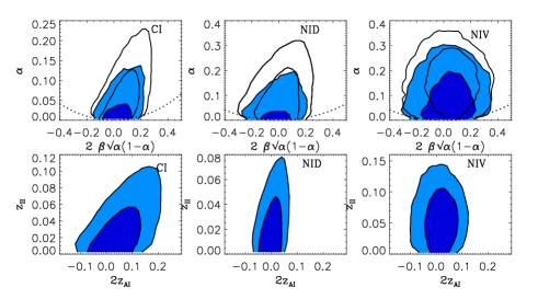
Figure 2: 68 % and 95 % 2-dimensional constraints on the amplitudes of generally correlated isocurvature modes, for the CI mode (left), the NID mode (center), and the NIV mode (right) for WMAP plus SDSS and SNLS data. The top panels show primordial amplitude contributions in terms of $\alpha,\beta$, using flat priors on ${z_{ij}}$ (line contours) and $\alpha,\beta$ (filled contours). The {$\alpha,2\beta\sqrt{\alpha(1-\alpha)}$} parameter space is contained within a circle of unit radius shown by the dashed line. The lower panels show the observable CMB power contributions in terms of ${z_{ij}}$.

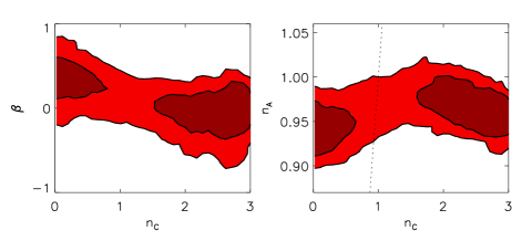
Figure 3: The effect of varying the CDM isocurvature spectral index independently for an AD+CI scenario with WMAP plus SDSS and SNLS data: 68 % and 95 % constraints on the AD-CI cross-correlation $\beta$ (left panel), and adiabatic spectral index (right panel). The dotted line in the right panel shows $n_{adi}=n_{iso}$.

The data is fully consistent with $\alpha=0/r_{iso}=0$, with the goodness of fit $-2\ln{\cal L}$ improved by only $\sim 1$ for each case. These additional degrees of freedom, however, cause the baryon density and spectral index mean values to move more than $1\sigma$ from their adiabatic values: both values are increased by $2\sigma$ when the NIV mode is included, exploiting the degeneracy observed in Bucher:2004an .

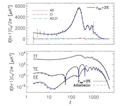
Figure 4: AD+CI: (Top) CMB temperature power spectrum for the best-fit model with correlated AD+CI modes and independent spectral indices (solid) for WMAP plus SDSS and SNLS data. The model has $r_{iso}=3.4\%$, $\alpha=0.49$, $\beta=-0.26$, $n_{adi}=0.97$, $n_{iso}=2.7$, and has $-2\ln{\cal L}$ lower than the best-fit adiabatic model. The contribution of each mode correlation to the total spectrum is shown, including the WMAP data. Bottom: the CMB spectra are compared to the pure adiabatic best-fit model (dashed). Only the $\ell<500$ section of the TE spectrum is shown.

Our investigation finds that the results are sensitive to the choice of prior: constraints on $\alpha$ obtained by sampling $\alpha$ and $\beta$ directly differ from those derived from the distribution sampled using the $z_{ij}$ parameterization. This is demonstrated in the top row of Figure 2, where the two methods are compared. We see that there is more phase space available for models with larger $\alpha$ when sampling with a uniform prior on the observable isocurvature CMB power, than there is when sampling with a uniform prior on $\alpha$. The likelihood of the best-fitting models are not affected by the choice of prior however, and we can expect the dependence to be reduced as data improves.

If the assumption of $n_{iso}=n_{adi}$ is relaxed, and $n_{iso}$ is allowed to vary freely within the bounds $0<n_{iso}<3$, a large phase space is opened up for models with large $n_{iso}$, within the range allowed by the prior. The 1-D marginalized constraints on the isocurvature contribution are increased from $r_{iso}<0.13$ to $<0.15$ (95% c.l.). The isocurvature tilt cannot be constrained by WMAP+SDSS+SN1a datasets alone, however Beltran:2005gr show that additional Ly-$\alpha$ data prefer higher tilts of $1.9\pm 1$. When spectral indices are able to vary freely, $r_{iso}$ is a good measure of isocurvature because $\alpha$ then becomes extremely sensitive to the pivot point at which the spectral indices are defined. The scenario we investigate here with CDM isocurvature and $n_{iso}\neq n_{adi}$ is a case in point. For models with high $n_{iso}(0.05/Mpc)$ the isocurvature power on larger cosmological scales is significantly reduced for a given $\alpha$ and therefore $\alpha$ is able to be increased to compensate. The relative power in isocurvature, however, roughly indicated by $\sim\alpha/(1-\alpha)\times(k/k_{0})^{n_{iso}-n_{adi}}$, is not increased.

The best-fit model is shown in Figure 4, has $n_{adi}=0.97$, $n_{iso}=2.7$ and may be distinguished from the adiabatic model at large scales in polarization. The goodness of fit is improved, compared to the adiabatic model, by a $\Delta(-2\ln{\cal L})$ of 4 to $11379$ for 2 additional degrees of freedom. Such an improvement is driven by the use of the 3-year WMAP data in the analysis. Future measurements will help distinguish these, currently degenerate, high isocurvature tilt models.

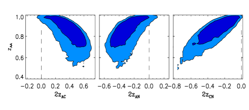
Figure 5: AD+CI+NID: 2-dimensional constraints show the degeneracy between isocurvature cross-correlation amplitudes $z_{ij}$, and the adiabatic amplitude $z_{AA}$, that allows the destructive interference of isocurvature spectra.

This subset of models may inform us about double inflation scenarios. If there are multiple fields driving inflation, it is possible to generate entropy perturbations in which the additional light fields modify the curvature perturbations on horizon scales, and also modify the consistency relations relating scalar to tensor modes Bartolo:2001rt ; Wands:2002bn . In the most general case $n_{adi}\neq n_{iso}\neq n_{corr}$, with each related to the slow roll parameters along the flat directions of the scalar fields. For example, for theories in which one scalar field plays a dominant role in driving inflation, but two fields play a significant role during reheating, one finds that $n_{iso}\approx n_{corr}$ Wands:2002bn . Analyses in which $n_{corr}$ has been allowed to vary have found it is a nuisance parameter unconstrained by data beltran:04 , so we believe it is reasonable to assume that fixing the scale dependence of the cross spectrum , $n_{corr}=(n_{adi}+n_{iso})/2$, does not unduly bias the conclusion. For two field inflation of two minimally coupled scalar fields of mass $m_{h}$ and $m_{l}$, the magnitude and correlation of the resulting CDM isocurvature component are dependent on the ratio of the masses $R=m_{h}/m_{l}$ and number of e-foldings $s_{k}$. A bound on $R$ comes from the magnitude of the cross-correlated spectrum beltran:04

$$2\beta\sqrt{\alpha(1-\alpha)}|_{max} = \frac{2s_{k}(R^{2}-1)}{s_{k}^{2}+(R^{2}+1)^{2}}$$ (11)

Assuming $s_{k}=60$ we find an upper bound on the ratio of the two scalar fields of $R<3.5$. This is weaker than the $R<3$ at 95% c.l. obtained with the inclusion of Lyman-$\alpha$ data Beltran:2005gr , although we caution that constraints on $\alpha$ in this case are strongly dependent on the choice of prior and pivot scale.

It would be interesting, but beyond the scope of this paper, to place constraints on specific double inflation models in which model-dependent predictions for each mode’s spectral index are included.

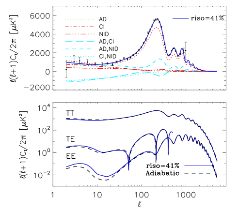
Figure 6: AD+CI+NID: Spectra as in Figure 4. The model shown has correlated modes, with $r_{iso}=41\%$, and cosmological parameters $\Omega_{b}h^{2}=0.026$, $\Omega_{c}h^{2}=0.12$, $\Omega_{\Lambda}=0.73$, $\tau=0.10$, $n_{s}=0.92$, $b_{SDSS}=0.98$. The isocurvature spectra add destructively, canceling almost completely.

V Generally correlated isocurvature: multiple modes

In this section we consider models with two additional correlated isocurvature modes, (CI+NID, CI+NIV, NID+NIV), and finally a model with the full set of adiabatic and three isocurvature modes. We sample the modes using the parameterization given in equation (7) for $N=3$ and $N=4$. Table 2 shows constraints for the relative mode contributions for this set of models. We also give the primordial amplitudes ${\cal A}_{ii}$ of the auto-correlations contributing to the best-fitting models, where $C_{\ell}=\sum_{i,j=1}^{N}{\cal A}_{ij}C_{\ell}^{ij}$.

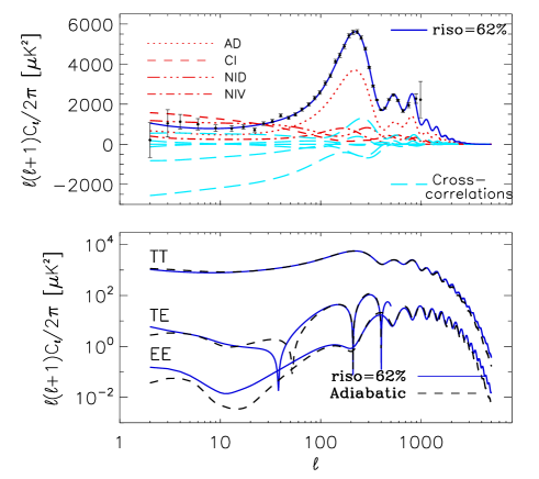
Figure 7: AD+CI+NID+NIV: Spectra as in Figure 4. The model shown has $r_{iso}=62\%$. No BBN or bias constraint has been imposed; the cosmological parameters are $\Omega_{b}h^{2}=0.037$, $\Omega_{c}h^{2}=0.13$, $\Omega_{\Lambda}=0.75$, $\tau=0.10$, $n_{s}=0.98$, $b_{SDSS}=1.2$.

Two isocurvature modes: As is shown in Table 2, models with two modes permit far more isocurvature than those with a single mode.

Although when considered individually, the neutrino velocity isocurvature modes allow the largest isocurvature fraction, interestingly when two modes are included, joint CDM and neutrino density isocurvature (CI+NID) allow the most freedom, more than twice as much isocurvature ($r_{iso}=0.4\pm 0.1$) as the combinations including the neutrino velocity mode. This freedom arises from degeneracies within the isocurvature components destructively interfering, originally observed in Moodley:2004nz and shown in Figure 5. Degeneracies with the NIV mode do also exist where the spectra add constructively, but such models have large baryon densities ruled out by current BBN measurements.

Figure 6 shows the best-fit CMB temperature spectrum for the CDM + neutrino density isocurvature model with $r_{iso}=41\%$, compared with 47% with WMAP year 1 data Moodley:2004nz . The contributions from all six correlations (three auto-correlations and three cross-correlations) lead to greater large scale polarization CMB power, but cancel almost completely in the CMB temperature and galaxy power spectrum.

All three two-mode models prefer baryon densities higher than the concordance value (with mean values $0.025<\Omega_{b}h^{2}<0.027$), despite the BBN constraint. The spectral index is also more poorly constrained, with the CI+NID models preferring a low spectral index ($0.93\pm 0.03$), and the CI+NIV ($0.99\pm 0.04$) and NID+NIV ($1.03\pm 0.03$) preferring larger values. The other cosmological parameters are consistent with adiabatic $\Lambda$ CDM.

Three isocurvature modes: When all three modes are included, the constraints are highly sensitive to the BBN constraint due to the strong degeneracy between $\Omega_{b}h^{2}$ and the NIV amplitude. With the BBN prior and SDSS bias we find $r_{iso}=0.44\pm 0.09$, increasing to $r_{iso}=0.51\pm 0.09$ when no BBN or SDSS bias priors are included, to be compared to $0.57\pm 0.09$ found for the first year WMAP data Bucher:2004an .

A well-fitting model ($\Delta$($-2\ln{\cal L}$)=-6 with 10 extra degrees of freedom in comparison to the adiabatic best fit) with a majority of the power coming from isocurvature modes, $r_{iso}=62\%$, is shown in Fig. 7. This model was obtained without the BBN prior and has a large baryon density ($\Omega_{b}h^{2}=0.037$); however even including the BBN constraint, the baryon density is higher than the concordance value for this class of models ($0.031\pm 0.003$), and $\Omega_{c}h^{2}$ is raised by $1\sigma$ to $0.124\pm 0.007$. Figures 6 and 7 indicate that precision small-scale temperature and large-scale polarization will to more tightly determine the underlying initial conditions. In particular future small-scale CMB experiments should strengthen the constraint on the baryon density, since high baryonic isocurvature models are more degenerate at smaller scales than their low baryon counterparts.

Given that the data can still only poorly constrain the isocurvature contribution for these multi-mode models, the constraints presented here depend on the prior distribution we have chosen. Previous work has shown that other parameterizations can decrease or increase this contribution Moodley:2004nz , depending on the phase-space volume available for purely adiabatic models compared to mixed isocurvature models. As with the single mode case, improved data will help limit this prior dependency.

VI Conclusion

	CI+NID	CI+NIV	NID+NIV		CI+NID+NIV	CI+NID+NIV
						No BBN/bias
$r_{\mbox{\scriptsize iso}}$	$0.4\pm 0.1$	$0.15\pm 0.06$	$0.20\pm 0.08$		$0.44\pm 0.09$	$0.51\pm 0.09$
$z_{AA}$	$0.8\pm 0.1$	$0.98\pm 0.02$	$0.96\pm 0.03$		$0.8\pm 0.1$	$0.7\pm 0.1$
$z_{CC}$	$0.2\pm 0.1$	$0.04\pm^{0.03}_{0.02}$	$-$		$0.21\pm 0.09$	$0.23\pm 0.09$
$z_{NN}$	$0.16\pm 0.09$	$-$	$0.05\pm 0.03$		$0.23\pm 0.09$	$0.28\pm 0.10$
$z_{VV}$	$-$	$0.09\pm 0.05$	$0.17\pm 0.09$		$0.15\pm 0.06$	$0.21\pm 0.09$
$10^{10}{\cal A}_{AA}$	$18.1$	$21.8$	$20.0$		$20.0$	$14.1$
$10^{10}{\cal A}_{CC}$	$5.2$	$0.45$	$-$		$11.2$	$12.4$
$10^{10}{\cal A}_{NN}$	$8.1$	$-$	$0.35$		$34.9$	$37.2$
$10^{10}{\cal A}_{VV}$	$-$	$3.0$	$4.7$		$8.9$	$21.4$
Added dof	$4$	$4$	$4$		$8$	$10$
$-2\ln{\cal L}$ ($\Delta(-2\ln{\cal L})$)	$11379(-4)$	$11382(-1)$	$11381(-2)$		$11375(-8)$	$11374(-9)$

Table 2: Means and $68\%$ c.l. for auto-correlated contributions ($z_{ij}$) for models with generally correlated isocurvature modes as indicated. The best-fit primordial amplitudes ${\cal A}_{ii}$ for the pure modes are shown.

We have investigated the constraints on the presence of a variety of isocurvature modes in the initial conditions of structure formation, in light of recent observations of temperature and polarization CMB data and large scale structure and supernovae surveys.

The improved WMAP data, with the inclusion of low $l$ polarization measurements, has strengthened these constraints on the contributions of individual isocurvature modes, with the polarization data disfavoring models with a large isocurvature fraction. Scenarios with either CDM (or baryon) or neutrino isocurvature allow only a very limited contribution, which can be translated into strong constraints on the curvaton model and some double-field inflationary models. Although models with multiple isocurvature modes do not offer a significantly better fit to the data, models with non-zero isocurvature fluctuations fit the data as well as the adiabatic model and can comprise the majority of power when additional modes are considered simultaneously.

Of the models with more than one isocurvature mode, those most likely to pose the greatest difficulty for distinguishing with future data are those with large fractions of both correlated CDM and neutrino density isocurvature, which provide the best fit to the data, and due to their destructive interference are highly degenerate in the CMB and galaxy power spectra. Those with neutrino velocity fluctuations (both two and three mode models) are better constrained by BBN and bias measurements.

With WMAP plus LSS and SN data, the baryon density and spectral tilt are found to be sensitive to the inclusion of isocurvature modes. With the current data, the reionization optical depth however is robust despite the modifications isocurvature models can make to large scale polarization spectra. Extending beyond the $\Lambda$ CDM scenario, given results found in dunkley , we would not expect that allowing independent tilts for all the modes, or including curved geometries, to have a large effect. Future B-mode polarization data will help break degeneracies between tensor and isocurvature modes that would currently arise from large scale temperature CMB data.

Future small-scale temperature and polarization data, together with improved galaxy and Lyman-$\alpha$ power spectrum measurements, should help constrain a subset of the models we have considered, but improved large scale CMB polarization data from WMAP and in particular Planck, demonstrated in Bucher:2002 , will be crucial if we are to strongly constrain this general set of correlated isocurvature models.

References

- (1) G. Hinshaw et al., arXiv:astro-ph/0603451.
- (2) N. Jarosik et al., arXiv:astro-ph/0603452.
- (3) L. Page et al., arXiv:astro-ph/0603450.
- (4) D. N. Spergel et al., arXiv:astro-ph/0603449.
- (5) W. J. Percival et al., Mon, Not. R. Astron. Soc, 327, 1297 (2001).
- (6) M. Tegmark et al. [SDSS Collaboration], Astrophys. J. 606, 702 (2004) [arXiv:astro-ph/0310725].
- (7) U. Seljak et al., Phys. Rev. D 71, 043511 (2005) [arXiv:astro-ph/0406594].
- (8) D. J. Eisenstein et al., Astrophys. J. 633, 560 (2005) [arXiv:astro-ph/0501171].
- (9) S. Cole et al. [The 2dFGRS Collaboration], Mon. Not. Roy. Astron. Soc. 362 (2005) 505 [arXiv:astro-ph/0501174].
- (10) A. G. Riess et al. [Supernova Search Team Collaboration], Astrophys. J. 607, 665 (2004) [arXiv:astro-ph/0402512].
- (11) P. Astier et al., arXiv:astro-ph/0510447.
- (12) U. Seljak et al., [arXiv:astro-ph/0604335].
- (13) D. Polarski and A. A. Starobinsky, Phys. Rev. D 50, 6123 (1994) [arXiv:astro-ph/9404061];
- (14) J. Garcia-Bellido and D. Wands, Phys. Rev. D 53, 5437 (1996) [arXiv:astro-ph/9511029];
- (15) A. D. Linde and V. Mukhanov, Phys. Rev. D 56, 535 (1997) [arXiv:astro-ph/9610219];
- (16) E. Pierpaoli, J. Garcia-Bellido and S. Borgani, JHEP 9910, 015 (1999) [arXiv:hep-ph/9909420];
- (17) M. Kawasaki and F. Takahashi, Phys. Lett. B 516, 388 (2001) [arXiv:hep-ph/0105134]
- (18) R. A. Battye and J. Weller, Phys. Rev. D 61, 043501 (2000) [arXiv:astro-ph/9810203].
- (19) R. A. Battye, J. Magueijo and J. Weller, arXiv:astro-ph/9906093.
- (20) D. H. Lyth and D. Wands, Phys. Lett. B 524, 5 (2002) [arXiv:hep-ph/0110002].
- (21) T. Moroi and T. Takahashi, Phys. Lett. B 522, 215 (2001) [Erratum-ibid. B 539, 303 (2002)] [arXiv:hep-ph/0110096].
- (22) N. Bartolo and A. R. Liddle, Phys. Rev. D 65, 121301 (2002) [arXiv:astro-ph/0203076].
- (23) T. Moroi and T. Takahashi, Phys. Rev. D 66, 063501 (2002) [arXiv:hep-ph/0206026].
- (24) D. H. Lyth, C. Ungarelli and D. Wands, Phys. Rev. D 67, 023503 (2003) [arXiv:astro-ph/0208055].
- (25) K. Dimopoulos, G. Lazarides, D. Lyth and R. Ruiz de Austri, JHEP 0305, 057 (2003) [arXiv:hep-ph/0303154].
- (26) K. Dimopoulos, D. H. Lyth, A. Notari and A. Riotto, JHEP 0307, 053 (2003) [arXiv:hep-ph/0304050].
- (27) V. Bozza, M. Gasperini, M. Giovannini and G. Veneziano, Phys. Lett. B 543, 14 (2002) [arXiv:hep-ph/0206131]
- (28) J. R Bond and G. Efstathiou, Mon. Not. R. Astron. Soc. 22, 33 (1987); P. J. E. Peebles, Nature 327, 210 (1987);
- (29) A. Rebhan and D. Schwarz, Phys. Rev. D 50, 2541 (1994); A. Challinor and A. Lasenby, Astrophys. J. 513, 1 (1999), 531 (1999);
- (30) M. Bucher, K. Moodley and N. Turok, Phys. Rev. D. 62, 083508 (2000).
- (31) R. Stompor, A. J. Banday and K. M. Gorski, Astrophys. J. 463, 8 (1996) [arXiv:astro-ph/9511087].
- (32) D. Langlois and A. Riazuelo, Phys. Rev. D 62, 043504 (2000) [arXiv:astro-ph/9912497].
- (33) K. Enqvist, H. Kurki-Suonio and J. Valiviita, Phys. Rev. D 62, 103003 (2000) [arXiv:astro-ph/0006429]
- (34) L. Amendola, C. Gordon, D. Wands and M. Sasaki, Phys. Rev. Lett. 88, 211302 (2002) [arXiv:astro-ph/0107089].
- (35) H. V. Peiris et al., Astrophys. J. Suppl. 148, 213 (2003) [arXiv:astro-ph/0302225].
- (36) J. Valiviita and V. Muhonen, Phys. Rev. Lett. 91, 131302 (2003) [arXiv:astro-ph/0304175].
- (37) P. Crotty et al., Phys. Rev. Lett. 91, 171301 (2003);
- (38) C. Gordon and K. A. Malik, Phys. Rev. D 69, 063508 (2004) [arXiv:astro-ph/0311102].
- (39) M. Beltran, J, Garc a-Bellido, J. Lesgourgues and A. Riazuelo, Phys. Rev. D. 70, 103530 (2004);
- (40) K. Moodley, M. Bucher, J. Dunkley, P. G. Ferreira and C. Skordis, Phys. Rev. D 70, 103520 (2004) [arXiv:astro-ph/0407304].
- (41) H. Kurki-Suonio, V. Muhonen and J. Valiviita, Phys. Rev. D 71, 063005 (2005) [arXiv:astro-ph/0412439].
- (42) M. Beltran, J. Garcia-Bellido, J. Lesgourgues and M. Viel, Phys. Rev. D 72, 103515 (2005) [arXiv:astro-ph/0509209].
- (43) M. Bucher, J. Dunkley, P. G. Ferreira, K. Moodley and C. Skordis, Phys. Rev. Lett. 93, 081301 (2004) [arXiv:astro-ph/0401417].
- (44) J. Dunkley, M. Bucher, P. G. Ferreira, K. Moodley and C. Skordis, Phys. Rev. Lett. 95, 261303 (2005)
- (45) A. Lewis, arXiv:astro-ph/0603753.
- (46) R. E. Smith et al., Mon, Not. R. Astron. Soc, 341, 1311 (2003).
- (47) G. Steigman, Int. J. Mod. Phys.,E15 (2006)
- (48) http://camb.info; A. Lewis, A. Challinor and A. Lasenby, Astrophys. J. 538, 473 (2000).
- (49) J. Dunkley, M. Bucher, P. G. Ferreira, K. Moodley and C. Skordis, Mon, Not. R. Astron. Soc, 356, 925 (2005).
- (50) A. Gelman and D. Rubin, Statistical Science 7, 457 (1992)
- (51) C. Gordon and A. Lewis, Phys. Rev. D 67, 123513 (2003) [arXiv:astro-ph/0212248].
- (52) N. Bartolo, S. Matarrese and A. Riotto, Phys. Rev. D 64, 123504 (2001) [arXiv:astro-ph/0107502].
- (53) D. Wands, N. Bartolo, S. Matarrese and A. Riotto, Phys. Rev. D 66, 043520 (2002) [arXiv:astro-ph/0205253].
- (54) M. Bucher, K. Moodley and N. Turok, Phys. Rev. Lett. 87, 191301 (2001); Phys. Rev. D. 66, 023528 (2002)