Neutrino emission due to Cooper pairing in neutron stars

Abstract

Neutrino emission caused by Cooper pairing of baryons in neutron stars is recalculated by accurately taking into account for conservation of the vector weak current. The vector current contribution to the neutrino emissivity is found to be several orders of magnitude smaller than that obtained before by different authors. Therefore, the neutrino energy losses due to singlet-state pairing of baryons can in practice be neglected in simulations of neutron star cooling. This makes negligible the neutrino radiation from pairing of protons or hyperons. The neutrino radiation from triplet pairing takes place through axial weak currents. For these states, when the total momentum projection is $m_{j}=0$, the vanishing of the vector weak current contribution results in the suppression of the neutrino energy losses by about 25%. The neutrino emissivity due to triplet pairing with $\left|m_{j}\right|=2$ is suppressed by about a factor of 3, caused by the collective contribution of spin-density fluctuations in the condensate.

1 Introduction

Thermal excitations in superfluid baryon matter of neutron stars, in the form of broken Cooper pairs, can recombine into the condensate by emitting neutrino pairs via neutral weak currents. The neutrino energy losses caused by the pairing of neutrons in a singlet state was first calculated by Flowers et al. [1] and reproduced by other authors [2], [3]. Yakovlev et al. [3] have also considered the neutrino energy losses in the case of neutron pairing in a triplet state. Jaikumar & Prakash [4] have generalized this mechanism to superconducting quark matter. The neutrino energy losses due to pairing of hyperons [5], [6] are also discussed in the literature as possible cooling mechanisms for superdense baryonic matter in neutron stars. Nowadays, these ideas are widely accepted and used in numerical simulations of neutron star evolution [7], [8], [9]. Nevertheless, the existing theory of neutrino radiation from Cooper pairing of baryons (quarks) in neutron stars rises some questions because, as we show below, it is inconsistent with the hypothesis of conservation of the vector current in weak interactions.

Let us recall shortly the main steps in the above calculations. The low-energy Lagrangian of the weak interaction may be described by a point-like current-current approach. For interactions mediated by neutral weak currents, it can be written as

$$\mathcal{L}_{vac}=\frac{G_{F}}{2\sqrt{2}}J_{B}^{\mu}l_{\mu}.$$ (1)

Here $G_{F}$ is the Fermi coupling constant, and the neutrino weak current is given by $l_{\mu}=\bar{\nu}\gamma_{\mu}\left(1-\gamma_{5}\right)\nu$. The vacuum weak current of the fermion (baryon or quark) is of the form $J_{\mu}=\bar{\psi}\left(C_{V}\gamma_{\mu}-C_{A}\gamma_{\mu}\gamma_{5}\right)\psi$, where, $\psi$ represents the fermion field, and the weak vertex includes the vector and axial-vector terms with the corresponding coupling constants $C_{V}$ and $C_{A}$.

Since relativistic calculations are more complicated and less transparent, we consider the nonrelativistic case, typical for superfluid baryon matter in neutron stars. Then, the nonrelativistic limits for the baryon operators are $\bar{\psi}_{B}\gamma^{0}\psi_{B}\rightarrow\hat{\Psi}_{B}^{+}\hat{\Psi}_{B}$, $\bar{\psi}_{B}\gamma_{i}\gamma_{5}\psi_{B}\rightarrow\hat{\Psi}_{B}^{+}\hat{\sigma}_{i}\hat{\Psi}_{B}$, all others being zero. Here $\hat{\Psi}_{B}$ is the second-quantized nonrelativistic spinor wave function, and $\hat{\sigma}_{i}$ are the Pauli matrices.

The process is kinematically allowed due to the existence of a superfluid energy gap $\Delta$, which admits the transition with time-like momentum transfer $K=\left(\omega,\mathbf{k}\right)$, as required by the final neutrino pair. We have $\omega>2\Delta$ and $\omega>k$ . The emissivity for neutrino pairs due to recombination of baryon quasi-particle excitations in the singlet state is then

$$Q = \left(\frac{G_{F}}{2\sqrt{2}}\right)^{2}C_{V}^{2}\int\frac{d^{3}pd^{3}p^{\prime}}{\left(2\pi\right)^{8}}f\left(\epsilon_{\mathbf{p}}\right)f\left(\epsilon_{\mathbf{p}^{\prime}}\right)\int\frac{d^{3}k_{1}}{2\omega_{1}}\frac{d^{3}k_{2}}{2\omega_{2}}\omega\left|\mathcal{M}_{B}\right|^{2}\left|\mathcal{M}_{\nu}\right|^{2}$$ (2)

$$\times\delta\left(\mathbf{p+p}^{\prime}-\mathbf{k}\right)\delta\left(\epsilon_{\mathbf{p}}+\epsilon_{\mathbf{p}^{\prime}}-\omega\right).$$

Here $\omega=\omega_{1}+\omega_{2}$ and $\mathbf{k=k}_{1}+\mathbf{k}_{2}$ are the energy and momentum carried out by the freely escaping neutrino pair, and $f\left(\epsilon_{p}\right)$ is the Fermi distribution function of the quasi-particles with energy $\epsilon_{p}$, as given by Eq. (17). The neutrino matrix element is of the standard form $\left|\mathcal{M}_{\nu}\right|^{2}=8\left(\omega_{1}\omega_{2}-\mathbf{k}_{1}\mathbf{k}_{2}\right)$. Therefore, the relevant input for this calculation is the recombination matrix element between the baryon state, which has a pair of quasi-particle excitations of momentum-spin labels $\left(\mathbf{p},\mathrm{up};\mathbf{p}^{\prime},\mathrm{down}\right)$, and the same state but with these excitations restored to the condensate. To the leading (zero) order in $k\ll p_{F}$, this matrix element is usually estimated as

$$\left|\mathcal{M}_{B}\right|^{2}=\frac{\Delta^{2}}{\epsilon_{p}^{2}}$$ (3)

yielding the following neutrino energy losses at temperature $T<T_{c}$.

$$Q_{\mathrm{FRS}}\left({}^{1}S_{0}\right)=\frac{4G_{F}^{2}{p}_{F}M^{\ast}C_{V}^{2}}{15\pi^{5}}\mathcal{N}_{\nu}T^{7}y^{2}\int_{0}^{\infty}\;\frac{z^{4}dx}{\left(e^{z}+1\right)^{2}},$$ (4)

where $M^{\ast}$ is the effective nucleon mass, $y=\Delta/T$, $z=\sqrt{x^{2}+y^{2}}$, and $\mathcal{N}_{\nu}=3$ is the number of neutrino flavors. $T_{c}$ is the critical temperature for baryon pairing.

The naive estimate (3) is inconsistent with the hypothesis of conservation of the vector current in weak interactions. Indeed, a longitudinal vector current of quasi-particles consisting only on a temporal component can not satisfy the continuity equation.

The question of conservation of the longitudinal vector current caused by recombination of quasi-particles has been discussed by many people [10] in connection with the gauge invariance of the Bardeen-Cooper-Schrieffer theory of superconductivity. It was realized that the current conservation could be restored if the interaction among quasi-particles is incorporated in the coupling vertex to the same degree of approximation as the self-energy effect is included in the quasi-particle. It has been also pointed out that there is significant difference between the transverse and longitudinal current operators in their matrix elements. Namely, there exist collective excited states of quasi-particle pairs [11], [12] which can be excited only by the longitudinal current. As a result, the spatial part of the longitudinal current does not vanish, and cancels the temporal part.

In the present paper we recalculate the neutrino energy losses with allowance for conservation of the weak vector current. The paper is organized as follows. In section 2 we shortly discuss the Nambu-Gorkov formalism as a convenient description of the particle-hole excitations in the system with pairing. The wave functions of the quasi-particle excitations are obtained in section 3. In section 4 we derive an effective vertex conserving the vector weak current for neutral and charged baryons. In section 5 we use the quasi-particle states for the calculation of the matrix element of the effective vector weak current, and the neutrino energy losses in the vector channel. The neutrino energy losses in the axial channel are calculated in section 6. A discussion of the obtained results and our main conclusions are presented in section 7.

2 Formalism

In the Nambu-Gorkov formalism, the quasi-particle fields are represented by two-component objects

$$\Psi_{p}=\left(\begin{array}[]{c}\psi_{\mathbf{1}}\left(p\right)\\ \psi_{2}^{\dagger}\left(-p\right)\end{array}\right)$$ (5)

$\psi_{\mathbf{1}}\left(p\right)$ is the the quasi-particle component of the excitation with momentum $\mathbf{p}$ and spin $\sigma$, and $\psi_{2}^{\dagger}\left(-p\right)$ is the hole component of the same excitation, which can be interpreted as the absence of a particle with momentum $-\mathbf{p}$ and spin $-\sigma$. The two-component fields (5) obey the standard fermion commutation relations

$$\left\{\Psi_{p,\sigma},\Psi_{p^{\prime},\sigma^{\prime}}\right\}=\delta_{\sigma,\sigma^{\prime}}\delta_{p,p^{\prime}}.$$

With the aid of the $2\times 2$ Pauli matrices

$$\hat{\tau}_{1}=\left(\begin{array}[]{cc}0&1\\ 1&0\end{array}\right),\ \hat{\tau}_{2}=\left(\begin{array}[]{cc}0&-i\\ i&0\end{array}\right),\ \hat{\tau}_{3}=\left(\begin{array}[]{cc}1&0\\ 0&-1\end{array}\right)$$ (6)

operating in the particle-hole space, the Hamiltonian of the system of quasi-particles can be recast as [12]

$$H=H_{0}+H_{1},$$

where

$$H_{0}=\sum_{p}\Psi_{p}^{\dagger}\left(\xi_{\mathbf{p}}\hat{\tau}_{3}+\hat{\Lambda}\left(\mathbf{\check{p}}\right)\right)\Psi_{p}$$ (7)

is the BCS reduced Hamiltonian, where the nonrelativistic energy is measured relatively to the Fermi level

$$\xi_{\mathbf{p}}\equiv\frac{p^{2}}{2M^{\ast}}-\mu,$$

$M^{\ast}$ is the effective mass of the quasi-particle and $\mu$ is the Fermi energy. The quasi-particle self-energy, of the form

$$\hat{\Lambda}\left(\mathbf{\check{p}}\right)\equiv\left(\begin{array}[]{cc}0&\hat{D}\left(\mathbf{\check{p}}\right)\\ \hat{D}^{\dagger}\left(\mathbf{\check{p}}\right)&0\end{array}\right),$$ (8)

is a $2\times 2$ matrix in the Nambu-Gorkov space, and a $2\times 2$ matrix in the spin space, which depends on the orientation of the quasi-particle momentum $\mathbf{\check{p}}=\mathbf{p}/\left|\mathbf{p}\right|$ (see e.g. [15]).

The residual interaction among quasi-particles is given by the following Hamiltonian

$$H_{1}=\frac{1}{2}\sum_{p,p^{\prime}}V_{pp^{\prime}}\left(q\right)\left(\Psi_{p+q}^{\dagger}\hat{\tau}_{3}\Psi_{p}\right)\left(\Psi_{p^{\prime}-q}^{\dagger}\hat{\tau}_{3}\Psi_{p\prime}\right).$$

As follows from the Hamiltonian (7), the inverse of the quasi-particle propagator has the simple form:

$$i\text{\c{G}}^{-1}\left(p\right)=p_{0}-\xi_{\mathbf{p}}\hat{\tau}_{3}-\hat{\Lambda}\left(\mathbf{\check{p}}\right)$$ (9)

3 Quasi-particle states

Near the Fermi-surface, the imaginary part of the quasi-particle energy is small. Therefore, to the extent that the single-particle picture makes some physical sense, we will describe the quasi-particles with the aid of wave-functions. The states of quasi-particles obey the equation

$$\text{\c{G}}^{-1}\Psi_{\mathbf{p}}=0.$$ (10)

Writing $\Psi_{\mathbf{p}}$ in the form

$$\Psi_{\mathbf{p}}\equiv\frac{1}{\sqrt{N}}\left(\begin{array}[]{c}\alpha\\ \beta\end{array}\right)$$ (11)

with $\alpha$ and $\beta$ being two-component spinors, we arrive to the following set of matrix equations

$$\left(p_{0}-\xi_{p}\right)\alpha-\hat{D}\beta = 0$$

$$\hat{D}^{\dagger}\alpha-\left(p_{0}+\xi_{p}\right)\beta = 0$$

From the second equation we have

$$\alpha=\left(p_{0}+\xi_{p}\right)\left(\hat{D}^{\dagger}\right)^{-1}\beta$$ (12)

By substituting this into the first equation and multiplying $\hat{D}^{\dagger}$ from the left, we obtain

$$\left(p_{0}^{2}-\xi_{p}^{2}-\hat{D}^{\dagger}\hat{D}\right)\beta=0$$ (13)

This equation has nontrivial solutions only if

$$\det\left|p_{0}^{2}-\xi_{p}^{2}-\hat{D}^{\dagger}\hat{D}\right|=0.$$ (14)

In the interesting cases of singlet- and triplet-state pairing we are going to consider, the gap matrix $\hat{D}$ is proportional to the unitary matrix $\hat{\Upsilon}\left(\mathbf{\check{p}}\right)$

$$\hat{D}\left(\mathbf{\check{p}}\right)=\Delta_{\mathbf{\check{p}}}\hat{\Upsilon}\left(\mathbf{\check{p}}\right)$$ (15)

with $\Delta_{\mathbf{\check{p}}}$

a scalar function [15], so that

$$\hat{\Upsilon}^{\dagger}\hat{\Upsilon}=1$$ (16)

Eq. (14) then gives us the eigenvalues

$$p_{0}=\pm\epsilon_{\mathbf{p}},\ \ \ \ \epsilon_{\mathbf{p}}\equiv\sqrt{\xi_{p}^{2}+\Delta_{\mathbf{\check{p}}}^{2}}$$ (17)

with

$$\Delta_{\mathbf{\check{p}}}^{2}=\frac{1}{2}Tr\hat{D}^{\dagger}\hat{D}$$ (18)

Using the fact that Eq. (13) is diagonal, we may choose two independent solutions for $\beta$ as the ordinary spinors:

$$\beta_{1}^{\pm}=\chi_{\uparrow}\equiv\left(\begin{array}[]{c}1\\ 0\end{array}\right),\ \ \ \beta_{2}^{\pm}=\chi_{\downarrow}\equiv\left(\begin{array}[]{c}0\\ 1\end{array}\right)$$ (19)

Here, the upper sign corresponds to the positive- or negative-frequency solution, in accordance with Eq. (17). The $\alpha$-component of these solutions is to be found from Eq. (12).

From Eq. (15), we obtain

$$\left(\hat{D}^{\dagger}\right)^{-1}=\Delta_{\mathbf{\check{p}}}^{-1}\hat{\Upsilon}\left(\mathbf{\check{p}}\right)$$

Substitution this into Eq. (12) gives

$$\alpha_{i}^{\pm}=\Delta_{\mathbf{\check{p}}}^{-1}\left(\pm\epsilon_{\mathbf{p}}+\xi_{p}\right)\hat{\Upsilon}\beta_{i}$$ (20)

Making use of Eqs. (19), (20) we can find the normalized wave functions. The positive-frequency states can be written as

$$\Psi_{\mathbf{p},\sigma}=\frac{1}{\sqrt{N}}\left(\begin{array}[]{c}\Delta_{\mathbf{\check{p}}}^{-1}\left(\epsilon_{\mathbf{p}}+\xi_{p}\right)\hat{\Upsilon}\chi_{\sigma}\\ \chi_{\sigma}\end{array}\right)e^{i\mathbf{pr}-i\epsilon_{\mathbf{p}}t}.$$ (21)

The factor $1/\sqrt{N}$, in Eq. (11) is to be found from the normalization condition $\Psi_{\mathbf{p}}^{\dagger}\Psi_{\mathbf{p}}=1$. A direct evaluation making use of Eq. (16) yields

$$\frac{1}{\sqrt{N}}=\sqrt{\frac{\epsilon_{p}-\xi_{p}}{2\epsilon_{p}}}.$$

Incorporating this factor into Eq. (21) we obtain the positive-frequency eigenstates

$$\Psi_{\mathbf{p},\sigma}=\left(\begin{array}[]{c}u_{\mathbf{p}}\hat{\Upsilon}\chi_{\sigma}\\ v_{\mathbf{p}}\chi_{\sigma}\end{array}\right)e^{i\mathbf{pr}-i\epsilon_{\mathbf{p}}t}$$ (22)

with

$$u_{\mathbf{p}}=\sqrt{\frac{\epsilon_{p}+\xi_{p}}{2\epsilon_{p}}},\ \ \ \ v_{\mathbf{p}}=\sqrt{\frac{\epsilon_{p}-\xi_{p}}{2\epsilon_{p}}}.$$ (23)

The negative-frequency wave-functions can be obtained in the same way. The state with momentum $\mathbf{p}$ and spin-label $\sigma$ has the form

$$\Psi_{-\mathbf{p},-\sigma}=\left(\begin{array}[]{c}-v_{\mathbf{p}}\hat{\Upsilon}\chi_{-\sigma}\\ u_{\mathbf{p}}\chi_{-\sigma}\end{array}\right)e^{-i\mathbf{pr}+i\epsilon_{\mathbf{p}}t}$$ (24)

This solution is connected to the hole state by the particle-antiparticle conjugation

$$C:\ \Psi^{C}=C\Psi^{\dagger}=\hat{\tau}_{2}\Psi^{\dagger}.$$

which changes quasi-particles of energy-momentum $\left(p_{0},\mathbf{p}\right)$ into holes of energy-momentum $\left(-p_{0},-\mathbf{p}\right)$, or interchanges up-spin and down-spin particles.

It is necessary to note that, in general, $\Psi_{\mathbf{p},\sigma}$ is not an eigenstate of the spin projection, because the upper component $\propto\hat{\Upsilon}\chi_{\sigma}$ is a linear combination of different spin states. The label $\sigma$ indicates only the spin function of the lower component, and serves for identification of the quasi-particle states.

4 Effective vertex for quasi-particles

4.1 Neutral baryons

The components of the bare vertex

$$\gamma^{\mu}=\left\{\begin{array}[]{cc}\hat{\tau}_{3}&\mathrm{if\ }\mu=0,\\ \frac{1}{M^{\ast}}\mathbf{p}&\mathrm{if\ }\mu=i=1,2,3\end{array}\right..$$ (25)

are $2\times 2$ matrices in the Nambu-Gorkov space. As already mentioned, the longitudinal current corresponding to the bare vertex does not satisfy the continuity equation. To restore the current conservation, one must consider the modification of the vertex $\gamma^{\mu}$ to the same order as the modification of the propagator is done. The relation between the modified vertex $\Gamma^{\mu}$ and the quasi-particle propagator (9) is given by the Ward identity [13]

$$K_{\mu}\Gamma^{\mu}\left(p^{\prime},p\right)=\hat{\tau}_{3}\text{\c{G}}^{-1}\left(p\right)-\text{\c{G}}^{-1}\left(p^{\prime}\right)\hat{\tau}_{3},$$ (26)

where $K=\left(\omega,\mathbf{k}\right)$ is the transferred momentum. The plane wave solutions

$$u_{\mathbf{p},\alpha}\exp\left(i\mathbf{pr}-i\epsilon_{\mathbf{p}}t\right),\ \ \ \ \ u_{\mathbf{p}^{\prime},\alpha^{\prime}}^{\ast}\exp\left(-i\mathbf{pr}+i\epsilon_{\mathbf{p}}t\right)$$

for $\Psi$ and $\Psi^{+}$ obey the equations Ģ${}^{-1}\left(p\right)u_{\mathbf{p},\alpha}=0$, and $u_{\mathbf{p}^{\prime},\alpha^{\prime}}^{\ast}$Ģ${}^{-1}\left(p^{\prime}\right)=0$. Therefore the Ward identity implies conservation of the vector current on the energy shell of the quasi-particles.

Following the prescriptions of quantum electrodynamics, an approximation which satisfies the Ward identity (and hence the continuity equation) is the sum of ladder diagrams satisfying the Dyson equation shown in Fig. 1.

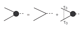
Figure 1: Dyson equation, in the ladder approximation, for the effective vertex. Solid lines stand for dressed particles, and the dashed line represents the $Z$-boson field. The wavy line accounts for the residual interaction among quasi-particles.

In these diagrams, all solid lines are "dressed" particles, and the dashed line is the $Z$-boson field. The "dressed" particles interact with the same primary interaction $V_{pp^{\prime}}$ which produces the self-energy of the quasi-particle. Thus, for $K=p-p^{\prime}$, the corrected vertex satisfies the integral equation

$$\Gamma^{\mu}\left(p-K,p\right) = \hat{\gamma}^{\mu}\left(p-K,p\right)$$

$$+i\int\frac{d^{4}p^{\prime}}{\left(2\pi\right)^{4}}\ \hat{\tau}_{3}\text{\c{G}}\left(p^{\prime}-K\right)\Gamma^{\mu}\left(p^{\prime}-K,p^{\prime}\right)\text{\c{G}}\left(p^{\prime}\right)\hat{\tau}_{3}V_{pp^{\prime}}$$

In the limit $K=\left(\omega,\mathbf{0}\right)$, the Ward identity gives

$$\Gamma^{0}\left(p-K,p\right)=\hat{\tau}_{3}-\frac{2}{\omega}\hat{\tau}_{3}\hat{\Lambda}\left(\mathbf{\check{p}}\right)$$

with

$$\hat{\tau}_{3}\hat{\Lambda}\left(\mathbf{\check{p}}\right)=\left(\begin{array}[]{cc}0&\hat{D}\left(\mathbf{\check{p}}\right)\\ -\hat{D}^{\dagger}\left(\mathbf{\check{p}}\right)&0\end{array}\right)$$ (28)

The poles of the vertex function correspond to collective eigen-modes of the system. Therefore, the pole which appears at $\omega\rightarrow 0$, $k=0$ implies the existence of a collective mode, which plays an important role in the conservation of the vector current. The corresponding nonperturbative solution to Eq. (4.1) has been found by Nambu [12] (see also [14]). In our notation, it reads

$$\Gamma_{0}\left(p-K,p\right)=\hat{\tau}_{3}-2\hat{\tau}_{3}\hat{\Lambda}\left(\mathbf{\check{p}}\right)\frac{\omega}{\omega^{2}-a^{2}k^{2}}$$ (29)

$$\mathbf{\Gamma}=\frac{\mathbf{p}}{M}-2\hat{\tau}_{3}\hat{\Lambda}\left(\mathbf{\check{p}}\right)\frac{a^{2}\mathbf{k}}{\omega^{2}-a^{2}k^{2}},$$ (30)

The poles in this vertex correspond to the collective motion of the condensate, with the dispersion relation $\omega=ak$, where $a^{2}=V_{F}^{2}/3$.

The effective vertex satisfies the Ward identity (26), and thus the continuity equation on the energy shell

$$\omega\Gamma_{0}-\mathbf{k\Gamma}\simeq 0$$ (31)

Indeed, by making use of $\omega=\epsilon_{\mathbf{p}}+\epsilon_{\mathbf{p}^{\prime}}$ and $\mathbf{k}=\mathbf{p}+\mathbf{p}^{\prime}$ with $\ k\ll p\simeq p_{F}$, the left-hand side of this equation can be reduced to the right-hand side of the Ward identity (26).

4.2 Charged baryons

Consider now the case when quasi-particles carry an electric charge. Including the long-range Coulomb interaction $V_{C}\left(k\right)=e^{2}/k^{2}$ implies that the vertex part is multiplied by a string of closed loops, which represents the polarization of the surrounding medium. In this case, the new vertex $\tilde{\Gamma}^{\mu}$ can be found as the solution of the Dyson equation, according to the diagram of Fig. 2. or, analytically

$$\tilde{\Gamma}^{\mu}\left(p-K,p\right) = \Gamma^{\mu}\left(p-K,p\right)-\Gamma_{0}\left(p-K,p\right)V_{C}\left(k\right)$$ (32)

$$\times i\int\frac{d^{4}p^{\prime}}{\left(2\pi\right)^{4}}\ Tr\left[\hat{\tau}_{3}\text{\c{G}}\left(p^{\prime}-K\right)\tilde{\Gamma}^{\mu}\left(p^{\prime}-K,p^{\prime}\right)\text{\c{G}}\left(p^{\prime}\right)\right]$$

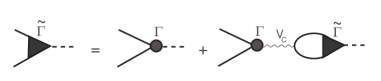
Figure 2: Dyson equation for the vertex correction for charged quasi-particles (compare with Fig. 1). The shaded areas represent the modified effective vertex, and the wavy line stands for the Coulomb interaction.

The integral

$$\tilde{\Pi}^{0\mu}\left(K\right)\equiv i\int\frac{d^{4}p^{\prime}}{\left(2\pi\right)^{4}}\ Tr\left[\hat{\tau}_{3}\text{\c{G}}\left(p^{\prime}-K\right)\tilde{\Gamma}^{\mu}\left(p^{\prime}-K,p^{\prime}\right)\text{\c{G}}\left(p^{\prime}\right)\right]$$ (33)

in the r.h.s. of Eq. (32) represents the $\tilde{\Pi}^{0\mu}$ component of the polarization tensor shown by the loop in Fig. 2. Introducing also the notation

$$\Pi^{0\mu}\left(K\right)\equiv i\int\frac{d^{4}p^{\prime}}{\left(2\pi\right)^{4}}\ Tr\left[\hat{\tau}_{3}\text{\c{G}}\left(p^{\prime}-K\right)\Gamma^{\mu}\left(p^{\prime}-K,p^{\prime}\right)\text{\c{G}}\left(p^{\prime}\right)\right]$$

Eq. (32) can be recast as follows

$$\tilde{\Pi}^{0\mu}\left(K\right)=\Pi^{0\mu}\left(K\right)-V_{C}\left(k\right)\Pi^{00}\left(K\right)\tilde{\Pi}^{0\mu}\left(K\right).$$

We then obtain

$$\tilde{\Pi}^{0\mu}\left(K\right)=\frac{\Pi^{0\mu}\left(K\right)}{1+V_{C}\left(k\right)\Pi^{00}\left(K\right)}.$$

Combining this with Eqs. (32), (33) yields

$$\tilde{\Gamma}^{\mu}\left(p-K,p\right)=\Gamma^{\mu}\left(p-K,p\right)\left(1-\frac{V_{C}\left(k\right)\Pi^{0\mu}\left(K\right)}{1+V_{C}\left(k\right)\Pi^{00}\left(K\right)}\right).$$

In particular, for $\Gamma^{0}$ we arrive to

$$\tilde{\Gamma}^{0}\left(p-K,p\right)=\frac{\Gamma^{0}\left(p-K,p\right)}{1+V_{C}\left(k\right)\Pi^{00}\left(K\right)}.$$ (34)

The polarization function $\Pi^{00}\left(K\right)$ can be readily calculated with the help of $\Gamma^{0}$ given by Eq. (29). By neglecting the small dependence of the energy gap on the transferred momentum $\mathbf{k}$, we have

$$\Pi^{00}\left(K\right) = i\int\frac{d^{4}p^{\prime}}{\left(2\pi\right)^{4}}\ Tr\left[\hat{\tau}_{3}\text{\c{G}}\left(p^{\prime}-K\right)\hat{\tau}_{3}\text{\c{G}}\left(p^{\prime}\right)\right]$$

$$-\frac{2\omega}{\omega^{2}-a^{2}k^{2}}i\int\frac{d^{4}p^{\prime}}{\left(2\pi\right)^{4}}\ Tr\left[\hat{\tau}_{3}\text{\c{G}}\left(p^{\prime}-K\right)\hat{\tau}_{3}\hat{\Lambda}\left(p^{\prime}\right)\text{\c{G}}\left(p^{\prime}\right)\right].$$

Here the quasi-particle propagator follows from Eq. (9):

$$\text{\c{G}}\left(p\right)=\frac{i}{p_{0}^{2}-\epsilon_{p}^{2}}\left(p_{0}+\xi_{p}\hat{\tau}_{3}+\hat{\Lambda}\left(\mathbf{\check{p}}\right)\right)$$ (35)

Performing the trace over particle-hole and spin indices, and integration over $p_{0}$, results in the following expression

$$\Pi^{00}\left(\omega,\mathbf{k}\right) = \int\frac{2d^{3}p}{\left(2\pi\right)^{3}}\ \frac{\omega\epsilon_{\mathbf{p}-\mathbf{k}}-\Delta_{\mathbf{\check{p}}}^{2}-\xi_{\mathbf{p}}\xi_{\mathbf{p-k}}-\epsilon_{\mathbf{p-k}}^{2}-a^{2}k^{2}\left(\omega^{2}-a^{2}k^{2}\right)^{-1}2\Delta_{\mathbf{\check{p}}}^{2}}{\epsilon_{\mathbf{p}-\mathbf{k}}\left(\omega-\epsilon_{\mathbf{p}}-\epsilon_{\mathbf{p-k}}\right)\left(\omega+\epsilon_{\mathbf{p}}-\epsilon_{\mathbf{p-k}}\right)}$$

$$+\int\frac{2d^{3}p}{\left(2\pi\right)^{3}}\ \frac{-\omega\epsilon_{\mathbf{p}}-\Delta_{\mathbf{\check{p}}}^{2}-\epsilon_{\mathbf{p}}^{2}-\xi_{\mathbf{p}}\xi_{\mathbf{p-k}}-a^{2}k^{2}\left(\omega^{2}-a^{2}k^{2}\right)^{-1}2\Delta_{\mathbf{\check{p}}}^{2}}{\epsilon_{\mathbf{p}}\left(\omega+\epsilon_{\mathbf{p}}+\epsilon_{\mathbf{p-k}}\right)\left(\omega-\epsilon_{\mathbf{p-k}}+\epsilon_{\mathbf{p}}\right)}$$

We are interested in the regime defined by

$$k<\omega,\ \ \ \omega>2\epsilon_{\mathbf{p}}\gg\epsilon_{\mathbf{p}}-\epsilon_{\mathbf{p-k}}\simeq kV_{F}$$

In this case we obtain, after some simplifications

$$\Pi^{00}\left(\omega,\mathbf{k}\right) = \frac{1}{8\pi^{3}}\left[\frac{a^{2}k^{2}}{\omega^{2}-a^{2}k^{2}}\int d^{3}p\ \frac{\Delta_{\mathbf{\check{p}}}^{2}}{\epsilon_{p}\left(\epsilon_{p}^{2}-a^{2}k^{2}/4\right)}\right.$$

$$\left.+k^{2}\int d^{3}p\ \frac{\Delta_{\mathbf{\check{p}}}^{2}}{\epsilon_{p}\left(\omega^{2}-4\epsilon_{p}^{2}\right)}\left(\frac{p^{2}}{3M^{2}\epsilon_{p}^{2}}-\frac{a^{2}}{\epsilon_{p}^{2}-a^{2}k^{2}/4}\right)\right].$$

with $a^{2}=V_{F}^{2}/3$.

Inserting this into Eq. (34) gives

$$\tilde{\Gamma}^{0}\left(p-K,p\right)=\frac{\Gamma^{0}\left(p-K,p\right)}{1+\chi\left(K\right)}$$ (36)

with

$$\chi\left(K\right) = \frac{e^{2}}{8\pi^{3}}\left[\frac{a^{2}}{\omega^{2}-a^{2}k^{2}}\int d^{3}p\ \allowbreak\frac{\Delta_{\mathbf{\check{p}}}^{2}}{\epsilon_{p}\left(\epsilon_{p}^{2}-a^{2}k^{2}/4\right)}\right.$$ (37)

$$\left.+\int d^{3}p\ \frac{\Delta_{\mathbf{\check{p}}}^{2}}{\epsilon_{p}\left(\omega^{2}-4\epsilon_{p}^{2}\right)}\allowbreak\left(\frac{p^{2}}{3M^{2}\epsilon_{p}^{2}}-\frac{a^{2}}{\epsilon_{p}^{2}-a^{2}k^{2}/4}\right)\right].$$

5 Energy losses in the vector channel

5.1 Neutral baryons

Having at hand the effective vertex and the wave functions of quasi-particles and holes, we can evaluate the matrix element of the vector weak current. In the particle-hole picture, the creation and recombination of two quasi-particles is described by the off-diagonal matrix elements of the Hamiltonian, which corresponds to quasi-particle transitions into a hole (and a correlated pair). Thus, we calculate the matrix element of the current between the initial (positive-frequency) state of a quasi-particle with momentum $\mathbf{p}$ and the final (negative-frequency) state with the same momentum $\mathbf{p}$.

$$\mathcal{M}_{\mu}=\left\langle\Psi_{-\mathbf{p,}-\sigma}^{\dagger}\left|\Gamma_{\mu}\right|\Psi_{\mathbf{p,\sigma}}\right\rangle$$

Let us consider separately the contributions from the bare vertex, given by the first terms in Eq. (29), and the collective part, given by the second term, so that $\mathcal{M}_{\mu}=\mathcal{M}_{\mu}^{\mathrm{bare}}+\mathcal{M}_{\mu}^{\mathrm{coll}}$.

Making use of the wave functions described by Eqs. (22), (24) and using the identity (16), for $\mu=0$, we find

$$\mathcal{M}_{0}^{\mathrm{bare}}=-\left(u_{p}v_{p^{\prime}}+v_{p}u_{p^{\prime}}\right)\simeq-\frac{\Delta_{\mathbf{\check{p}}}}{\epsilon_{p}},\ \ \ \ k\ll p\simeq p_{F}$$ (38)

$$\mathcal{M}_{0}^{\mathrm{coll}}=2\Delta_{\mathbf{\check{p}}}\frac{\omega}{\omega^{2}-a^{2}k^{2}}\left(u_{p}u_{p^{\prime}}+v_{p}v_{p^{\prime}}\right)\simeq 2\Delta_{\mathbf{\check{p}}}\frac{\omega}{\omega^{2}-a^{2}k^{2}}.$$

with $\epsilon_{p}+\epsilon_{p^{\prime}}=\omega$ and $\mathbf{p+p}^{\prime}=\mathbf{k}$.

The velocity of the collective mode $a^{2}=V_{F}^{2}/3$ is small in the nonrelativistic system. Therefore, we expand the collective contribution in this parameter to obtain

$$\mathcal{M}_{0}^{\mathrm{coll}}\simeq\frac{\Delta_{\mathbf{\check{p}}}}{\epsilon_{p}}\left(1+\frac{1}{3}V_{F}^{2}\frac{k^{2}}{\omega^{2}}\right)$$ (39)

The contribution of the bare vertex $\mathcal{M}_{0}^{\mathrm{bare}}$ reproduces the matrix element (3) derived by Flowers et al. [1] and Yakovlev et al. [3]. However, the collective correction modifies this crucially. In the sum of the two contributions, the leading terms mutually cancel, yielding the matrix element

$$\mathcal{M}_{0}=\mathcal{M}_{0}^{\mathrm{bare}}+\mathcal{M}_{0}^{\mathrm{coll}}\simeq\frac{1}{3}V_{F}^{2}\frac{k^{2}}{\omega^{2}}\frac{\Delta_{\mathbf{\check{p}}}}{\epsilon_{p}}$$

which is at least $\sim V_{F}^{2}$ times smaller than the bare result.

The above cancellation of the contribution of "bare" vertex is not accidental. This part of the matrix element, which remains finite at zero transferred momentum, cannot be restored with taking into account of more complicated corrections to the vertex part. It is well-known that, for any process involving interactions, the perturbation diagrams can be grouped into gauge invariant subsets, such that the invariance is maintained by each subset taken as a whole. If any new subset of the diagrams is added to the vertex part, the same should also be incorporated into the quasi-particle self-energy. If this is carefully done, for $k\rightarrow 0$, one must obtain the exact cancellation of the contribution of the "bare" vertex. Indeed, $\Psi^{+}\left(\mathbf{r},t\right)\Psi\left(\mathbf{r},t\right)$ represents the operator of baryon charge density. If the ground state $\left|0\right\rangle$ is an eigenstate of the baryon charge operator for the system with $N$ particles, and $|n>$ is a state for the system with $N+2$ particles, the matrix element

$$\int\left\langle 0\right|\Psi_{B}^{+}\left(\mathbf{r},t\right)\Psi_{B}\left(\mathbf{r},t\right)\left|n\right\rangle e^{i\mathbf{kr}-i\omega t}d^{3}rdt$$

should vanish for $k\rightarrow 0$, because the above expression is an off-diagonal matrix element of the total charge operator $Q$. This implies that, for $k\ll p_{F}$ , the matrix element should be proportional to some power of $k$.

The spatial component of the longitudinal (with respect to $\mathbf{k}$) component of the matrix element can be obtained from Eq. (31). Since $\mathbf{\check{k}\Gamma=}\left(\omega/k\right)\Gamma_{0}$ we have

$$\mathcal{M}_{\parallel}\simeq\frac{1}{3}V_{F}^{2}\frac{k}{\omega}\frac{\Delta_{\mathbf{\check{p}}}}{\epsilon_{p}}.$$

In the above, $\ \mathbf{\check{k}=k}/k$ is a unit vector directed along the transferred momentum.

Since the collective interaction modifies only the longitudinal part of the vertex, the transverse part of the matrix element can be evaluated directly from the bare vertex (25). This yields

$$\mathcal{M}_{\perp}\simeq\left(v_{p}u_{p^{\prime}}-u_{p}v_{p^{\prime}}\right)\frac{\mathbf{p}_{\perp}}{M^{\ast}}\simeq-\frac{1}{2}V_{F}^{2}\frac{k\Delta_{\mathbf{\check{p}}}}{\epsilon_{\mathbf{p}}^{2}}\left(\mathbf{\check{k}\check{p}}\right)\mathbf{\check{p}}_{\perp}.$$

The rate of the process is proportional to the square of the matrix element. This means that the vector current contribution to the neutrino energy losses is $V_{F}^{4}$ times smaller than estimated before. The corresponding neutrino emissivity in the vector channel can be evaluated with the aid of Fermi’s golden rule:

$$Q_{V} = \left(\frac{G_{F}}{2\sqrt{2}}\right)^{2}\frac{C_{V}^{2}}{\left(2\pi\right)^{8}}\mathcal{N}_{\nu}\int d^{3}pd^{3}p^{\prime}f\left(\epsilon_{\mathbf{p}}\right)f\left(\epsilon_{\mathbf{p}^{\prime}}\right)$$

$$\times\int\frac{d^{3}k_{1}}{2\omega_{1}}\frac{d^{3}k_{2}}{2\omega_{2}}\omega\mathrm{Tr}\left(l_{\mu}l_{\nu}^{\ast}\right)\mathcal{M}^{\mu}\mathcal{M}^{\nu}\delta\left(\mathbf{p+p}^{\prime}-\mathbf{k}\right)\delta\left(\epsilon_{\mathbf{p}}+\epsilon_{\mathbf{p}^{\prime}}-\omega\right).$$

One can simplify this equation by inserting $\int d^{4}K\ \delta^{\left(4\right)}\left(K-k_{1}-k_{2}\right)=1$. Then, the phase-space integrals for neutrinos are readily done with the aid of Lenard’s formula

$$\int\frac{d^{3}k_{1}}{2\omega_{1}}\frac{d^{3}k_{2}}{2\omega_{2}}\delta^{\left(4\right)}\left(K-k_{1}-k_{2}\right)\mathrm{Tr}\left(j^{\mu}j^{\nu\ast}\right)$$

$$= \frac{4\pi}{3}\left(K_{\mu}K_{\nu}-K^{2}g_{\mu\nu}\right)\Theta\left(K^{2}\right)\Theta\left(\omega\right),$$

where $\Theta(x)$ is the Heaviside step function.

For $k\ll p_{F}$ we obtain

$$Q_{V} = \frac{4\pi}{3}\left(\frac{G_{F}}{2\sqrt{2}}\right)^{2}\frac{C_{V}^{2}}{\left(2\pi\right)^{8}}\mathcal{N}_{\nu}\int d^{3}pf^{2}\left(\epsilon_{\mathbf{p}}\right)\int_{0}^{\infty}d\omega\omega\int_{0}^{\omega}dkk^{2}d\Omega_{k}$$

$$\times\left(\left(K_{\mu}\mathcal{M}^{\mu}\right)^{2}-K^{2}\mathcal{M}^{\mu}\mathcal{M}_{\mu}\right)\delta\left(2\epsilon_{\mathbf{p}}-\omega\right).$$

The next integrations are trivial. We get

$$Q_{V}=\frac{592}{42\,525\pi^{5}}V_{F}^{4}G_{F}^{2}C_{V}^{2}p_{F}M^{\ast}T^{7}y^{2}\int_{0}^{\infty}\;\frac{z^{4}dx}{\left(e^{z}+1\right)^{2}}$$

This is to be compared with Eq. (4). We see that

$$\frac{Q_{V}}{Q_{\mathrm{FRS}}\left({}_{1}S^{0}\right)}=\frac{148}{2835}V_{F}^{4}$$

i.e. the neutrino radiation via the vector weak currents in the nonrelativistic system $\left(V_{F}\ll 1\right)$ is suppressed by several orders of magnitude with respect to the predictions of Flowers et al. [1].

5.2 Charged baryons

If the paired baryons carry an electric charge, the effective vector vertex is given by Eqs. (36), (29) and (37). We are interested in the case $\omega>2\Delta_{\mathbf{\check{p}}}$ and $k<\omega$. Since $a\ll 1$ and $p\simeq p_{F}$, the second integral in Eq. (37) may be dropped. By neglecting also the small contributions from $a^{2}k^{2}\ll\epsilon_{p}^{2},\omega^{2}$ we get

$$\chi\left(K\right)=e^{2}\frac{a^{2}}{\omega^{2}}\int\ \allowbreak\frac{\Delta_{\mathbf{\check{p}}}^{2}}{\epsilon_{p}^{3}}\frac{d^{3}p}{\left(2\pi\right)^{3}}=\frac{1}{\omega^{2}}\frac{e^{2}n}{M^{\ast}}\int\frac{d\Omega_{\mathbf{p}}}{4\pi}\int_{0}^{\infty}\ \allowbreak\frac{\Delta_{\mathbf{\check{p}}}^{2}}{\epsilon_{p}^{3}}d\xi$$

where $n$ is the number of baryons per unit volume. Since

$$\int\frac{d\Omega_{\mathbf{p}}}{4\pi}\int_{0}^{\infty}\ \allowbreak\frac{\Delta_{\mathbf{\check{p}}}^{2}}{\epsilon^{3}}d\xi = \int\frac{d\Omega_{\mathbf{p}}}{4\pi}\int_{\Delta}^{\infty}\ \allowbreak\frac{\Delta_{\mathbf{\check{p}}}^{2}}{\epsilon^{2}}\frac{1}{\sqrt{\epsilon^{2}-\Delta_{\mathbf{\check{p}}}^{2}}}d\epsilon$$

$$= \int\frac{d\Omega_{\mathbf{p}}}{4\pi}\int_{1}^{\infty}\ \allowbreak\frac{1}{x^{2}}\frac{1}{\sqrt{x^{2}-1}}dx=1$$

we obtain

$$\chi\left(K\right)=\frac{\omega_{p}^{2}}{\omega^{2}},\ \ \ \ \omega_{p}^{2}=\frac{e^{2}n}{M^{\ast}}$$

This agrees with the plasma frequency for a free gas of charged particles.

The energy exchange in the medium goes naturally as the temperature scale. Therefore, the energy transferred to the radiated neutrino-pair is $\omega\sim T\leq T_{c}$, while the plasma frequency $\omega_{p}$ is typically much larger than the critical temperature for Cooper pairing. For instance, for a number density $n$ of the order of the nuclear saturation density $n_{0}\simeq 0.17$ fm and the effective mass of the baryon $M^{\ast}$ of the order of the bare nucleon mass, we obtain $\omega_{p}\sim 10\ MeV$, while the critical temperature for baryon pairing is about $1\ MeV$ or less. Under these conditions, we obtain

$$\tilde{\Gamma}^{0}\left(p-K,p\right)\simeq\frac{\omega^{2}}{\omega_{p}^{2}}\Gamma^{0}\left(p-K,p\right)\sim\frac{T_{c}^{2}}{\omega_{p}^{2}}\Gamma^{0}\left(p-K,p\right)$$

Thus, in superconductors, the vector current contribution to the neutrino radiation is suppressed additionally by a factor $\left(T_{c}^{2}/\omega_{p}^{2}\right)^{2}$: this is the plasma screening effect. The total suppression factor, due to both the current conservation and the plasma effects, is of the order

$$\left(T_{c}^{2}/\omega_{p}^{2}\right)^{2}V_{F}^{4}\lesssim 10^{-6}.$$

6 Energy losses in the axial channel

The neutrino energy losses in the axial channel can also be obtained with the aid of Fermi’s golden rule. After integration over the phase space of participating particles, this yields (see details in [3]):

$$Q_{A}=C_{A}^{2}\frac{4G_{F}^{2}{p}_{F}M^{\ast}}{15\pi^{5}}\mathcal{N}_{\nu}T^{7}R_{A},\ \ \ R_{A}=\frac{C_{A}^{2}}{8\pi}\int d\Omega\ \int_{0}^{\infty}dx\;\frac{z^{6}dx}{\left(e^{z}+1\right)^{2}}I.$$ (40)

Here $\mathcal{N}_{\nu}=3$ is the number of neutrino flavors, $z=\sqrt{x^{2}+\Delta_{\mathbf{\check{p}}}^{2}/T^{2}}$, and the outer integration is performed over the orientations of the nucleon momentum $\mathbf{p}$. The matrix elements of the axial current

$$\mathbf{A}\left(\mathbf{\check{p}},\eta\right)\mathbf{\equiv}\left\langle\Psi_{-\mathbf{p,}-\eta^{\prime}}^{\dagger}\left|\mathbf{\hat{A}}\right|\Psi_{\mathbf{p,\eta}}\right\rangle$$

come into this expression under the combination

$$I=I_{xx}+I_{yy}+I_{zz}$$ (41)

with

$$I_{ii}=\sum_{\eta\eta^{\prime}}A_{i}\left(\mathbf{\check{p}},\eta\right)A_{i}^{\ast}\left(\mathbf{\check{p}},\eta^{\prime}\right)$$

The collective mode considered in previous sections represents density oscillations of the condensate, and does not influence the axial weak vertex of a quasi-particle, if the average spin projection of the bound pair is zero. This happens in the singlet-state pairing and in triplet pairing with total momentum projection $m_{j}=0$. In these cases, the axial vertex may be taken in its bare form $A_{\mathrm{i}}^{bare}=\hat{\Sigma_{i}}$, where the spin operator

$$\hat{\Sigma_{i}}=\hat{\sigma_{i}}\hat{\tau}_{3}\equiv\begin{pmatrix}\hat{\sigma_{i}}&0\\ 0&-\hat{\sigma_{i}}\end{pmatrix},$$ (42)

with $\hat{\sigma_{i}}=\left(\hat{\sigma}_{x},\hat{\sigma}_{y},\hat{\sigma}_{z}\right)$ being the Pauli spin matrices, is defined according to the relation

$$\hat{\Sigma}_{z}\Psi_{\mathbf{p},\eta}=\eta\Psi_{\mathbf{p},\eta},$$

where

$$\Psi_{\mathbf{p},\eta}=\left(\begin{array}[]{c}u_{\mathbf{p}}\chi_{\eta}\\ v_{\mathbf{p}}\chi_{-\eta}\end{array}\right)$$

is the eigenstate with spin projection $s_{z}=\eta/2=\pm 1/2$ along the $Z$-axis.

A direct evaluation of the matrix elements of the bare axial vertex (42) for a quasi-particle transition into a hole by making use of the wave functions (22), (24) gives $I=0$ in the case of singlet pairing. For triplet pairing with $m_{j}=0$ we obtain

$$I_{xx}=I_{yy}=\frac{\Delta_{\mathbf{\check{p}}}^{2}}{\epsilon_{p}^{2}}\left(1-\cos 2\varphi\right),\ \ \ I_{zz}=2\frac{\Delta_{\mathbf{\check{p}}}^{2}}{\epsilon_{p}^{2}}$$

which, after averaging over the azimuthal angle $\varphi$ of the quasi-particle momentum $\mathbf{p}$, gives

$$I=4\frac{\Delta_{\mathbf{\check{p}}}^{2}}{\epsilon_{p}^{2}}.$$ (43)

This confirms the corresponding result obtained in [3].

In the case of a triplet-state pairing with maximal momentum projection $\left|m_{j}\right|=2$, we obtain a different result. In this case, the spin projection of the Cooper pair is conserved, and collective density oscillations of the condensate are accompanied by oscillations of the spin density, i.e. by the axial current. The corresponding gap matrix of the quasi-particles has the form $\hat{D}=\Delta_{\mathbf{\check{p}}}\hat{\Upsilon}\left(\mathbf{\check{p}}\right)$ with [15]

$$\hat{\Upsilon}\left(\mathbf{\check{p}}\right)=\left(\begin{array}[]{cc}-e^{i\varphi}&0\\ 0&e^{-i\varphi}\end{array}\right)=-\hat{\sigma}_{z}\cos\varphi-i\sin\varphi.$$

Therefore, the operator $\hat{\Sigma}_{z}$ commutes with the quasi-particle Hamiltonian $H_{0}=\xi_{\mathbf{p}}\hat{\tau}_{3}+\hat{\Lambda}\left(\mathbf{\check{p}}\right)$, where $\hat{\Lambda}$ is given by Eq. (8). This modifies the $z$-component of the axial vertex, which should be found from the equation

$$\hat{A}_{z}\left(p-K,p\right)=\hat{\tau}_{3}\hat{\sigma}_{z}+i\int\frac{d^{4}p^{\prime}}{\left(2\pi\right)^{4}}\ \hat{\tau}_{3}\text{\c{G}}\left(p^{\prime}-K\right)\hat{A}_{z}\left(p^{\prime}-K,p^{\prime}\right)\text{\c{G}}\left(p^{\prime}\right)\hat{\tau}_{3}V_{pp^{\prime}}.$$

After multiplication of this equation by $\hat{\sigma}_{z}$ from the right-hand side, and introducing the new function

$$\hat{B}\equiv\hat{A}_{z}\left(p-K,p\right)\hat{\sigma}_{z}$$ (44)

we arrive to the following equation

$$\hat{B}\left(p-K,p\right)=\hat{\tau}_{3}+i\int\frac{d^{4}p^{\prime}}{\left(2\pi\right)^{4}}\ \hat{\tau}_{3}\text{\c{G}}\left(p^{\prime}-K\right)\hat{B}\left(p^{\prime}-K,p^{\prime}\right)\hat{\sigma}_{z}\text{\c{G}}\left(p^{\prime}\right)\hat{\sigma}_{z}\hat{\tau}_{3}V_{pp^{\prime}}.$$

By using the fact that $\hat{\sigma}_{z}$ commutes with Ģ$\left(p^{\prime}\right)$, one can reduce this equation to the form

$$\hat{B}\left(p-K,p\right)=\hat{\tau}_{3}+i\int\frac{d^{4}p^{\prime}}{\left(2\pi\right)^{4}}\ \hat{\tau}_{3}\text{\c{G}}\left(p^{\prime}-K\right)\hat{B}\left(p^{\prime}-K,p^{\prime}\right)\text{\c{G}}\left(p^{\prime}\right)\hat{\tau}_{3}V_{pp^{\prime}}$$

which is identical to Eq. (4.1) for $\mu=0$. Then, the solution has a form analogous to Eq. (29). We obtain

$$\hat{B}\left(p-K,p\right)=\hat{\tau}_{3}-2\hat{\tau}_{3}\hat{\Lambda}\left(\mathbf{\check{p}}\right)\frac{\omega}{\omega^{2}-a^{2}k^{2}}.$$

From Eq. (44) we find

$$\hat{A}_{z}\left(p-K,p\right)=\hat{\tau}_{3}\hat{\sigma}_{z}-2\hat{\tau}_{3}\hat{\Lambda}\left(\mathbf{\check{p}}\right)\hat{\sigma}_{z}\frac{\omega}{\omega^{2}-a^{2}k^{2}},$$

or, in an explicit form:

$$\hat{A}_{z}\left(p-K,p\right)=\left(\begin{array}[]{cc}\hat{\sigma}_{z}&0\\ 0&-\hat{\sigma}_{z}\end{array}\right)-2\left(\begin{array}[]{cc}0&\hat{\sigma}_{z}\hat{\Upsilon}\\ -\hat{\sigma}_{z}\hat{\Upsilon}^{\dagger}&0\end{array}\right)\frac{\omega\Delta_{\mathbf{\check{p}}}}{\omega^{2}-a^{2}k^{2}}.$$

The transverse components of the axial vertex are not modified

$$\hat{A}_{x}=\hat{\tau}_{3}\hat{\sigma}_{x}=\left(\begin{array}[]{cc}\hat{\sigma}_{x}&0\\ 0&-\hat{\sigma}_{x}\end{array}\right),\ \ \ \hat{A}_{y}=\hat{\tau}_{3}\hat{\sigma}_{y}=\left(\begin{array}[]{cc}\hat{\sigma}_{y}&0\\ 0&-\hat{\sigma}_{y}\end{array}\right).$$

Direct evaluation of the matrix elements for $k\ll p_{F}$ gives, in this case:

$$A_{z}\left(\mathbf{\check{p}},\eta\right)\simeq-\eta\left(\frac{\Delta_{\mathbf{\check{p}}}}{\epsilon_{\mathbf{p}}}-\frac{2\Delta_{\mathbf{\check{p}}}\omega}{\omega^{2}-a^{2}k^{2}}\right)\delta_{-\eta^{\prime},\eta}\simeq\frac{1}{3}\eta V_{F}^{2}\frac{k^{2}}{\omega^{2}}\frac{\Delta_{\mathbf{\check{p}}}}{\epsilon_{p}}\delta_{-\eta^{\prime},\eta},$$

$$A_{x}\left(\mathbf{\check{p}},\eta\right)=-\frac{\Delta_{\mathbf{\check{p}}}}{2\epsilon_{p}}\left(1-e^{2\eta i\varphi}\right)\delta_{\eta,\eta^{\prime}},$$

$$A_{y}\left(\mathbf{\check{p}},\eta\right)=-\frac{\Delta_{\mathbf{\check{p}}}}{2\epsilon_{p}}i\left(1-e^{2\eta i\varphi}\right)\delta_{\eta,\eta^{\prime}}\left(\delta_{\uparrow,\eta}-\delta_{\downarrow,\eta}\right).$$

Due to the contribution of the collective mode, the matrix element $A_{z}$ is $V_{F}^{2}$ times smaller than $A_{x}$ and $A_{y}$ and, thus, can be neglected. After averaging over the azimuthal angle $\varphi$ of the quasi-particle momentum, we obtain

$$I\simeq I_{xx}+I_{yy}=2\frac{\Delta_{\mathbf{\check{p}}}^{2}}{\epsilon_{p}^{2}}.$$ (45)

Thus, in the case of ${}^{3}P_{2}$ pairing with total momentum projection $\left|m_{j}\right|=2$, the value of $I$, given by Eq. (45), is twice smaller, and the neutrino energy losses are proportionally suppressed.

7 Discussion and conclusions

We have considered the problem of conservation of the vector weak current in the theory of neutrino-pair radiation from Cooper pairing in neutron stars. The correction to the vector weak vertex is calculated within the same order of approximation as the quasi-particle propagator is modified by the pairing interaction in the system. This correction restores the conservation of the vector weak current in the quasi-particle transition into the paired state. As a result, in the nonrelativistic baryon system, the matrix element of the vector current is $V_{F}^{2}$ times smaller than previous estimations. This means that the vector weak current contribution to neutrino radiation caused by Cooper paring is $V_{F}^{4}$ times smaller than it was thought before. The vector weak current contribution from pairing of charged baryons is suppressed additionally by a factor $\sim\left(T_{c}^{2}/\omega_{p}^{2}\right)^{2}$ due to plasma screening. The total suppression factor due to both the current conservation and the plasma effects is of the order

$$\left(T_{c}^{2}/\omega_{p}^{2}\right)^{2}V_{F}^{4}\lesssim 10^{-6}.$$

In papers [16], [17], a special case of proton pairing has been considered which accounts for electron-proton correlations, resulting in an increasing of the neutrino emissivity. This, however, takes place only because of a very small weak vector coupling constant of the proton with respect to that for the electron. In our calculations, incorporation of the electron-proton correlations would result in the replacement of the vector weak coupling constant of the proton by a form-factor, which is proportional (to the leading order) to the electron coupling constant. This could enlarge the effective proton vector weak coupling to almost the same order of magnitude as that for neutrons. However, the cancellation of the temporal component of the transition current due to current conservation is much more stronger, and makes negligible the neutrino emission from the proton pairing even with taking into account the electron-proton correlations. Thus, the neutrino energy losses due to singlet-state pairing of baryons can, in practice, be neglected in simulations of neutron star cooling. This makes unimportant the neutrino radiation from pairing of protons or hyperons.

The neutrino radiation from triplet pairing occurs through the axial weak currents. In the case of ${}^{3}P_{2}$ pairing with total momentum projection $m_{j}=0$, the corresponding neutrino emissivity is given by

$$Q\left(m_{j}=0\right)=C_{A}^{2}\frac{8G_{F}^{2}{p}_{F}M^{\ast}}{15\pi^{5}}\mathcal{N}_{\nu}T^{7}F_{t},$$ (46)

with

$$F_{t}=\frac{1}{4\pi}\int d\Omega\ y^{2}\int_{0}^{\infty}dx\;\frac{\left(x^{2}+y^{2}\right)^{2}}{\left(e^{\sqrt{x^{2}+y^{2}}}+1\right)^{2}}.$$ (47)

This formula can be obtained directly from the corresponding expression suggested in [3] by omitting the contribution proportional to the vector weak coupling constant $C_{V}^{2}$. As a result, the corresponding neutrino energy losses are suppressed by about 25%

$$\frac{Q\left(m_{j}=0\right)}{Q_{\mathrm{YKL}}\left(m_{j}=0\right)}=\frac{2C_{A}^{2}}{C_{V}^{2}+2C_{A}^{2}}=\frac{3.17}{4.17}$$

with respect to those calculated in [3].

In the case of ${}^{3}P_{2}$ pairing with total momentum projection $\left|m_{j}\right|=2$, the neutrino energy losses in the axial channel are additionally suppressed due to the collective contribution of the spin-density fluctuations in the condensate:

$$Q\left(\left|m_{j}\right|=2\right)=C_{A}^{2}\frac{4G_{F}^{2}{p}_{F}M^{\ast}}{15\pi^{5}}\mathcal{N}_{\nu}T^{7}F_{t}.$$ (48)

Together with the vanishing of the vector contribution, the total suppression of the neutrino emissivity with respect to that obtained in [3] is about 3 times

$$\frac{Q\left(\left|m_{j}\right|=2\right)}{Q_{\mathrm{YKL}}\left(\left|m_{j}\right|=2\right)}=\frac{C_{A}^{2}}{C_{V}^{2}+2C_{A}^{2}}=\frac{1.58}{4.17}.$$

In this paper, we have considered the neutrino radiation from Cooper pairing in nonrelativistic baryon matter. It is clear from the above consideration, however, that conservation of the vector weak current has to be restored also in the theory of neutrino radiation from pairing of relativistic quarks [4]. This will be done in a future work.

Acknowledgments

This work has been supported by Spanish Grants AYA2004-08067-C01, FPA2005-00711 and GV2005-264.

10

References

- [1] E. Flowers, M. Ruderman, P. Sutherland, ApJ 205 (1976) 541.
- [2] D. N. Voskresensky, and A. V. Senatorov, Sov. J. Nucl. Phys. 45 (1987) 411.
- [3] D. G. Yakovlev, A. D. Kaminker, K. P. Levenfish, A&A 343 (1999) 650.
- [4] P. Jaikumar and M. Prakash, arXiv: astro-ph/0105225
- [5] S. Balberg, N. Barnea, Phys. Rev. 57C (1998) 409.
- [6] Ch. Schaab, S. Balberg, J. Schaffner-Bielich, ApJL (1998) 504, L99.
- [7] C. Shaab, D. Voskresensky, A. D. Sedrakian, F. Weber, M. K. Weigel A&A, 321 (1997) 591.
- [8] D. Page, In: Many Faces of Neutron Stars (eds. R. Buccheri, J. van Peredijs, M. A. Alpar. Kluver, Dordrecht, 1998) p. 538.
- [9] D. G. Yakovlev, A. D. Kaminker, K. P. Levenfish, In: Neutron Stars and Pulsars (ed. N. Shibazaki et al., Universal Akademy Press, Tokio, 1998) p. 195.
- [10] M. J. Buckingam, Nuovo cimento, 5 (1957) 1763; J. Bardeen, Nuovo cimento, 5 (1957) 1765; M. R Schafroth, Phys. Rev. 111 (1958) 72; P. W. Anderson, Phys. Rev. 110 (1958) 827; 112 (1958) 1900; G. Rickayzen, Phys. Rev. 111 (1958) 817; Phys. Rev. Lett. 2 (1959) 91; D. Pines and R. Schieffer, Nuovo cimento 10 (1958) 496; Phys. Rev. Lett. 2 (1958) 407; J. M Blatt and T. Matsubara, Progr. Theor. Phys. 20 (1958) 781.
- [11] N. N. Bogoliubov, Soviet Phys. 34 (1958) 41, 51.
- [12] Y. Nambu, Phys. Rev. 117 (1960) 648.
- [13] J. Schrieffer, Theory of Superconductivity (W. Benjamin, New York, 1964), p. 157.
- [14] P. B. Littlewood and C. M. Varma, Phys. Rev. B26 (1982) 4883.
- [15] R. Tamagaki, Progr. Theor. Phys. 44 (1970) 905.
- [16] L. B. Leinson, Phys. Lett. B473 (2000) 318.
- [17] L. B. Leinson, Nucl. Phys. A687 (2001) 489.