GaBoDS: The Garching-Bonn Deep Survey

Abstract

Aims. An interesting question of contemporary cosmology concerns the relation between the spatial distribution of galaxies and dark matter, which is thought to be the driving force behind the structure formation in the Universe. In this paper, we measure this relation, parameterised by the linear stochastic bias parameters, for a range of spatial scales using the data of the Garching-Bonn Deep Survey (GaBoDS).

Methods. The weak gravitational lensing effect is used to infer matter density fluctuations within the field-of-view of the survey fields. This information is employed for a statistical comparison of the galaxy distribution to the total matter distribution. The result of this comparison is expressed by means of the linear bias factor $b$, the ratio of density fluctuations, and the correlation factor $r$ between density fluctuations. The total galaxy sample is divided into three sub-samples using $R$-band magnitudes and the weak lensing analysis is applied separately for each sub-sample. Together with the photometric redshifts from the related COMBO-17 survey we estimate the typical mean redshifts of these samples with $\bar{z}=0.35,0.47,0.61$, respectively.

Results. Using a flat $\Lambda\rm CDM$ model with $\Omega_{\rm m}=0.3,\Omega_{\Lambda}=0.7$ as fiducial cosmology, we obtain values for the galaxy bias on scales between $1^{\prime}\leq\theta_{\rm ap}\leq 20^{\prime}$. At $10^{\prime}$, the median redshifts of the samples correspond roughly to a typical comoving scale of $3,5,7\leavevmode\nobreak\ h^{-1}\rm Mpc$ with $h=0.7$, respectively. We find evidence for a scale-dependence of $b$. Averaging the measurements of the bias over the range $2^{\prime}\leq\theta_{\rm ap}\leq 19^{\prime}$ yields $\bar{b}=0.81\pm 0.11,0.79\pm 0.11,0.81\pm 0.11$ ($1\sigma$), respectively. Galaxies are thus less clustered than the total matter on that particular range of scales (anti-biased). As for the correlation factor $r$ we see no scale-dependence within the statistical uncertainties; the average over the same range is $\bar{r}=0.61\pm 0.16,0.64\pm 0.18,0.58\pm 0.19$ ($1\sigma$), respectively. This implies a possible decorrelation between galaxy and dark matter distribution. An evolution of galaxy bias with redshift is not found, the upper limits are: $\Delta b\lesssim 0.2$ and $\Delta r\lesssim 0.4(1\sigma)$.

1 Introduction

In comparison to the total mass in the Universe, galaxies take – considering their mass – only a minor part in the big picture of structure formation. They formed from the baryonic component, embedded in the fluctuations of the dark matter density field, whose total mean density is very much lower than that of dark matter. Due to their relatively easy observability, it would be very convenient if galaxies were perfect tracers – unbiased tracers – of the total mass distribution; all statistical properties of the mass structure could then be derived from galaxy catalogues.

Indeed, it is rather unlikely that galaxies are unbiased tracers, because the laws determining the galaxy distribution are very complex and highly non-linear. The primordial gas from which they form requires special conditions to be able to cool and fragment into galaxies (White & Frenk 1991; White & Rees 1978). Due to shock heating of the baryons and energy feedback between galaxies and the intergalactic medium, the properties of the gas feeding galaxy formation gradually changed with time. Furthermore, galaxies interact with each other or with the baryonic intergalactic medium, merge or get accreted into more massive galaxies (Lacey & Cole 1993). These mechanisms probably produced the large diversity in galaxy masses, colours, morphologies and chemistry we observe today. Based on our current knowledge it would be very surprising if this complexity would eventually result in a simple, linear, one-to-one relationship between the galaxy density and total matter density, making galaxies unbiased tracers. But by studying this dark matter-galaxy relationship we can learn more about galaxies.

Observing the relation between the invisible dark matter field and the galaxies is a particularly tough problem. However, with gravitational lensing at hand, we now have a technique to directly unravel this relationship. The importance of “cosmic shear” as a tool for cosmology was proposed in the early 1990s by Blandford et al. (1991), Miralda-Escudé (1991) and Kaiser (1992). Since these pioneering days of gravitational lensing the techniques and surveys have been refined to make valuable contributions to the ongoing research on structure formation on cosmological scales. In particular, the investigation of the relation between galaxy and dark matter distribution using the weak gravitational lensing effect has become almost standard (Seljak et al. 2005; Kleinheinrich et al. 2005; Sheldon et al. 2004; Hoekstra et al. 2003; Guzik & Seljak 2001; McKay et al. 2001; Fisher et al. 2000; Hudson et al. 1998; Brainerd et al. 1996). This paper will focus on the lensing technique as well.

1.1 Quantifying galaxy bias

From the point of view of statistics, quantifying galaxy bias leads to the question how one can parametrise differences in the statistical properties – not the obvious differences between two particular realisations – of two random fields. Both the distribution of galaxies and the distribution of dark matter are thought to be realisations of statistically homogeneous and isotropic random fields. Commonly, one uses a parametric way to describe the biasing between two (random) density fields, for instance galaxy and matter distribution or the distributions of two different galaxy populations. Biasing between two density fields, say $\rho_{\rm g}$ and $\rho_{\rm m}$, can in general be quantified using the joint probability distribution function (PDF) $P\left(\delta_{\rm g},\delta_{\rm m}\right)$ of the density contrasts (density fluctuations)

$$\delta_{\rm g}\equiv\frac{\rho_{\rm g}}{\langle\rho_{\rm g}\rangle}-1\leavevmode\nobreak\ \leavevmode\nobreak\ ;\leavevmode\nobreak\ \leavevmode\nobreak\ \delta_{\rm m}\equiv\frac{\rho_{\rm m}}{\langle\rho_{\rm m}\rangle}-1$$ (1)

at the same point in the density fields at some redshift (local Eulerian bias). The probability of finding density contrasts of $\delta_{\rm g}$ and $\delta_{\rm m}$ within an interval of ${\rm d}\delta_{\rm g}$ and ${\rm d}\delta_{\rm m}$, respectively, equals $P(\delta_{\rm g},\delta_{\rm m}){\rm d}\delta_{\rm m}{\rm d}\delta_{\rm g}$. The density contrasts are smoothed to a certain scale, $R$, before investigating their PDF. Often the special type of smoothing kernel is set by the method that is used to determine the bias. To lowest, second order (first order moments vanish by definition, $\langle\delta_{\rm g}\rangle=\langle\delta_{\rm m}\rangle=0$) the only relevant parameters for biasing are the scale-dependent parameters of the “linear stochastic bias”

$$b(R)=\sqrt{\frac{\langle\delta_{\rm g}^{2}\rangle}{\langle\delta_{\rm m}^{2}\rangle}}\leavevmode\nobreak\ \leavevmode\nobreak\ ;\leavevmode\nobreak\ \leavevmode\nobreak\ r(R)=\frac{\langle\delta_{\rm g}\delta_{\rm m}\rangle}{\sqrt{\langle\delta_{\rm g}^{2}\rangle\langle\delta_{\rm m}^{2}\rangle}}\;,$$ (2)

which differ from unity in the case of two biased fields. These two parameters provide a complete description for the bias between $\delta_{\rm g}$ and $\delta_{\rm m}$ for Gaussian fields only and therefore are a full description only on large smoothing scales where linear perturbation theory applies (on “linear scales”). The linear bias factor $b$ is a measure for the difference in clustering strength. The correlation coefficient $r$, on the other hand, measures partly the stochasticity in the relation between the density contrasts, for instance how well minima and maxima of the density fields coincide. Only partly, because the correlation coefficient is also sensitive to the non-linearity in this relation, which becomes relevant on smaller smoothing scales where the fields are usually no longer Gaussian. In fact, they cannot be Gaussian since $\delta\geq-1$ by definition. Despite this degeneracy, the linear stochastic bias parameters are clearly defined on non-linear scales; it is just their interpretation which is no longer straightforward. To disentangle a non-linear but deterministic relation between two density contrasts from a stochastic one requires higher-order statistics, like for example in the context of the “non-linear stochastic bias” scheme (Dekel & Lahav 1999).

1.2 Galaxy bias in observations

Observationally, galaxy bias can be derived from the one-dimensional PDF of galaxies, $P(\delta_{\rm g})$, (Marinoni et al. 2005; Sigad et al. 2000), redshift space-distortions (Pen 1998; Kaiser 1987), weak gravitational lensing (Seljak et al. 2005; Sheldon et al. 2004; Pen et al. 2003; Hoekstra et al. 2002; Wilson et al. 2001; van Waerbeke 1998; Schneider 1998) and counts-in-cells statistics (Conway et al. 2005; Tegmark & Bromley 1999; Efstathiou et al. 1990). Additionally, the large-scale flow of galaxies can be used to make a POTENT reconstruction of the total mass field on large scales which can be compared to the galaxy distribution (Sigad et al. 1998; Dekel et al. 1993). Gravitational lensing (Schneider et al. 2006; van Waerbeke & Mellier 2003; Bartelmann & Schneider 2001) provides a promising new method in this respect because it allows for the first time to map the total matter content (mainly dark matter) independent from the galaxy distribution. The work of this paper is based on this technique.

A brief overview of the current status of the observational results is given in the following. Note that the given conclusions to some extent depend on the assumed cosmological model. We quote only the conclusions for the concordance $\Lambda\rm CDM$ model (cf. Tegmark et al. 2004). In the local universe, $L_{\star}$ galaxies are almost unbiased tracers on linear scales of about $8h^{-1}\rm Mpc$ and larger (Seljak et al. 2005; Verde et al. 2002; Lahav et al. 2002; Loveday et al. 1996). However, this is probably not true on smaller scales. A comparison of the theoretical dark matter clustering – which is constrained by the cosmic microwave background anisotropies, gravitational lensing and the Lyman-$\alpha$ forest (Tegmark et al. 2004) – and the observable galaxy clustering suggests that on smaller scales $\sim 1h^{-1}\rm Mpc$ galaxies are less clustered than the dark matter (“anti-biased”) becoming positively biased, $b>1$, on even smaller scales below $\sim 0.1h^{-1}\rm Mpc$. Hoekstra et al. (2001, 2002) use in their work on the VIRMOS-DESCART survey (van Waerbeke et al. 2001) and RCS (Gladders & Yee 2001) weak gravitational lensing to measure the linear stochastic bias for galaxies with a median redshift of $z_{\rm m}=0.35$, covering a range from $0.1h^{-1}{\rm Mpc}$ to $6.3h^{-1}{\rm Mpc}$. They claim to have observed such a dip in the linear bias factor. Also based on gravitational lensing there is evidence that the ratio $b/r$ stays close to unity from sub-megaparsec scales up to $\sim 8h^{-1}\rm Mpc$ (Sheldon et al. 2004; Hoekstra et al. 2002; Guzik & Seljak 2001; Fisher et al. 2000), thus from non-linear to linear scales. The analysis of the bispectrum of the galaxy clustering in the 2dFGRS (Colless et al. 2001) led Verde et al. (2002) to the conclusion that on scales between $5h^{-1}\rm Mpc$ and $30h^{-1}\rm Mpc$ the biasing relation between dark matter and galaxies is essentially linear (see also Lahav et al. 2002). The same conclusion was drawn several years earlier by Gaztańaga & Frieman (1994) based on the APM survey (Maddox et al. 1990). However, recently the work of Kayo et al. (2004) has questioned a strict linear relation on scales $\lesssim 10h^{-1}\rm Mpc$ by studying the three-point correlation of galaxy clustering as a function of morphology, colour and luminosity, this time in the SDSS (York et al. 2000).

Subdividing the galaxies into various subsets gives a more detailed picture of galaxy biasing. At low redshift, clustering is a function of morphological type, spectral type, colour and luminosity (e.g. Madgwick et al. 2003; Zehavi et al. 2002; Norberg et al. 2001; Benoist et al. 1996; Tucker et al. 1997; Loveday et al. 1995; Davis & Geller 1976). Late-type, blue, spiral or star forming galaxies are less clustered than early-type, elliptical or red galaxies with a relative linear bias factor of about $b_{\rm red}/b_{\rm blue}\approx 1.4$ on scales of roughly $8\,h^{-1}\rm Mpc$ (e.g. Wild et al. 2005; Conway et al. 2005; Zehavi et al. 2002; Norberg et al. 2002; Baker et al. 1998). On large scales, the relative biasing between red and blue galaxies does not seem to be well described by a simple linear biasing function which according to Wild et al. (2005) (see also Conway et al. 2005) is ruled out with high significance using counts-in-cells statistics in redshift space. Wild et al. observe a scale-dependent non-linear bias between red and blue galaxies with a dominant stochasticity component for typical physical scales of about $7h^{-1}\rm Mpc$ up to $31h^{-1}\rm Mpc$. Relative bias between red and blue galaxies is therefore both non-linear and stochastic. It is therefore also expected that at least for some galaxy populations the bias with respect to the dark matter distribution is non-linear and stochastic as suggested by simulations (Yoshikawa et al. 2001). This, however, has not been measured directly so far. Observational evidence for the relation between red and blue galaxies being non-deterministic was already given some years ago by the work of Tegmark & Bromley (1999), which was based on the Las Campas Redshift Survey (Shectman et al. 1996), and by Blanton (2000). Moreover, galaxy bias seems to be a function of redshift (Marinoni et al. 2005; Magliocchetti et al. 2000) which is expected both from simulations (Weinberg et al. 2004 and references therein) and analytical models (Tegmark & Peebles 1998; Mo & White 1996; Fry 1996).

In this paper, we apply the method of Hoekstra et al. (2002; Sect. 4) to the Garching-Bonn Deep Survey (Sect. 3) to obtain the linear stochastic bias coefficients $b$ and $r$ of three galaxy subsets binned by their apparent $R$-band magnitude. The selection of the galaxy samples is outlined in Sect. 3. After presenting our results in Sect. 5 we close with a discussion and conclusions in Sect. 6. We will start with a brief introduction to the formalism of weak gravitational lensing and the aperture statistics here employed.

Unless otherwise stated we use a $\Lambda$CDM model with $\Omega_{\rm m}=0.3$, $\Omega_{\Lambda}=0.7$ and $H_{0}=h\,100\,{\rm km}\,{\rm s}^{-1}\,{\rm Mpc}^{-1}$ with $h=0.7$. A scale-invariant ($n=1$, Harrison-Zel’dovich) spectrum of primordial fluctuations is assumed. As transfer function, encoding the physical properties of the cold dark matter fluid, we use Bardeen et al. (1986).

2 Formalism

2.1 Weak gravitational lensing

Weak gravitational lensing uses the shapes of distant galaxies – the source galaxies or, as we will also call them, background galaxies – to infer the distribution of the total matter. This is based on the fact that light is deflected by density fluctuations so that the tidal gravitational field of the matter density inhomogeneities along the line-of-side towards a galaxy changes the shape of its image. We consider only cases in which the light rays emitted from a source galaxy traverse only regions in space with relatively small perturbations in the gravitational field (weak lensing regime); this holds for almost every galaxy.

Theory.

In the weak lensing regime the differential distortion effect of the tidal gravitational field is well described by a two-dimensional linear mapping over the whole apparent size of one galaxy. The relevant components of the linear transformation ${\@tens{A}}$ are the convergence $\kappa$, which magnifies or demagnifies the size of a galaxy, and the shear, $\gamma\equiv\gamma_{1}+{\rm i}\gamma_{2}$, which stretches the image of a galaxy along some direction:

$${\@tens{A}}({\@vec{\theta}})=\left(\begin{array}[]{cc}1-\kappa-\gamma_{1}&-\gamma_{2}\\ -\gamma_{2}&1-\kappa+\gamma_{1}\end{array}\right)\;,$$ (3)

where ${\@vec{\theta}}$ is an angular position on the sky. Note that for convenience 2D vectors are written as complex numbers, as for instance ${\@vec{\theta}}=\theta_{1}+{\rm i}\theta_{2}$.

According to the theory of weak gravitational lensing, convergence and shear are, to lowest order, a projection of the three-dimensional density contrast $\delta_{\rm m}$ of the matter in the Universe via

$$\kappa({\@vec{\theta}}) = \int_{0}^{w_{\rm h}}{\rm d}w\,\overline{W}\left(w\right)\delta_{\rm m}(f_{\rm K}\left(w\right){\@vec{\theta}},w)\;,$$ (4)

$$\gamma({\@vec{\theta}}) = -\frac{1}{\pi}\int{\rm d^{2}}{\@vec{\theta}}^{\prime}\,\kappa({\@vec{\theta}}^{\prime}-{\@vec{\theta}})\frac{1}{(\theta_{1}^{\prime}-{\rm i}\theta_{2}^{\prime})^{2}}\;,$$ (5)

where

$$\overline{W}\left(w\right)=\frac{3\Omega_{\rm m}H_{0}^{2}f_{\rm K}\left(w\right)}{2c^{2}a\left(w\right)}\int_{w}^{w_{\rm h}}\!\!\!\!{\rm d}w^{\prime}\,p_{\rm b}\left(w^{\prime}\right)\frac{f_{\rm K}\left(w^{\prime}-w\right)}{f_{\rm K}\left(w^{\prime}\right)}$$ (6)

is a weight given to the density contrast at a comoving radial distance $w$ from the observer. The functions $a(w)$ and $f_{\rm K}(w)$ are the cosmic scale factor and the comoving angular distance, respectively, at comoving distance $w$. The variable $w_{\rm h}$ is the comoving horizon size. By $p_{\rm b}(w)$ we denote the distribution of the background sources in comoving distance. The shear $\gamma$ as a function of the direction on the sky ${\@vec{\theta}}$ is called the cosmic shear map. According to Eq. (5) it is a convolution of the convergence $\kappa$, thus the projected matter density contrast, with some kernel.

In the formalism presented here, we assume that we always observe only small patches of the celestial sphere; small enough to approximate the topology of the patch by a tangential, Cartesian plane (flat-sky approximation). This is a very good approximation for the survey fields considered here, which are smaller than $1\,\rm deg^{2}$. Furthermore, the 3D coordinate system, such as for $\delta_{\rm m}$ in Eq. (4), is chosen such that $w$ is a comoving distance along some fixed reference line-of-sight and $f_{\rm K}(w){\@vec{\theta}}$ a 2D-vector perpendicular to the reference line-of-sight; $w$ is also used as look-back time parameter to account for the fact that $\delta_{\rm m}$ is a function of time.

Connection to the real world.

To quantify the shape of a galaxy one defines the complex ellipticity, $\epsilon=\epsilon_{1}+{\rm i}\epsilon_{2}$, which is related to the quadrupole moments of the light distribution in the galaxy image (e.g. Schneider et al. 2006). It transforms under rotations according to $\epsilon^{\prime}=\exp{(-2{\rm i}\psi)}\,\epsilon$ where $\psi$ is the rotation angle.

Seitz & Schneider (1997), for example, showed that under the action of the linear transformation ${\@tens{A}}$ the intrinsic ellipticity, i.e. the unlensed galaxy ellipticity, $\epsilon_{\rm s}$, of a source galaxy is transformed into the image ellipticity, $\epsilon$, according to

$$\epsilon\approx\epsilon_{\rm s}+\gamma\;,$$ (7)

if $\gamma\ll 1$ which is fulfilled in the weak lensing regime. The practical importance of this equation stems from the fundamental assumption that galaxies have intrinsically no preferred direction and are therefore randomly oriented, i.e. $\langle\epsilon_{\rm s}\rangle=0$. This makes the observed ellipticities of galaxies, $\epsilon({\@vec{\theta}})$, unbiased estimators of the cosmic shear field in the direction ${\@vec{\theta}}$:

$$\langle\epsilon({\@vec{\theta}})\rangle=\gamma\left({\@vec{\theta}}\right)\;.$$ (8)

In this picture, the shear is a function of the convergence, and the convergence is related to the projected $\delta_{\rm m}$. Consequently, it should be possible to make a reconstruction of the total matter distribution based on the observed ellipticities of source galaxies, or a reconstruction of structural parameters such as spatial correlation functions.

Of course, galaxies are in general not intrinsically round objects, $\epsilon_{\rm s}\neq 0$; the ellipticities of single galaxies have typically $\left\langle|\epsilon_{\rm s}\right|\rangle\approx 0.3$ with a comparable scatter of $\sigma(|\epsilon_{s}|)\approx 0.3$. This makes them in fact very noisy estimators of the shear, considering that the shear signal induced by gravitational lensing is typically about one percent of this value. Therefore, the average over many galaxy ellipticities is required in weak lensing applications.

2.2 Aperture statistics

Aperture mass.

For our application here, which aims at the linear stochastic bias parameters on some smoothing scale, we are not interested in the convergence field itself but in the convergence field smoothed to some typical scale using an aperture filter $u$. A convenient quantity for this purpose is the aperture mass $M_{\rm ap}$ (Schneider et al. 1998) defined as

$$M_{\rm ap}\left(\theta_{\rm ap},{\@vec{\theta}}\right)\equiv\frac{1}{\theta^{2}_{\rm ap}}\int{\rm d}^{2}{\@vec{\theta}}^{\prime}\leavevmode\nobreak\ u\left(\frac{\left|{\@vec{\theta}}^{\prime}-{\@vec{\theta}}\right|}{\theta_{\rm ap}}\right)\kappa\left({\@vec{\theta}}^{\prime}\right)\;.$$ (9)

The variable $\theta_{\rm ap}$ is the aperture radius setting the filter scale. It has been shown that if the filter $u$ is compensated, $\int{\rm d}x\leavevmode\nobreak\ x\leavevmode\nobreak\ u\left(x\right)=0$, then the aperture mass can be determined from the shear field itself (Schneider 1996, 1998)

$$M_{{\rm ap}/\times}\left(\theta_{\rm ap},{\@vec{\theta}}\right)\!\! = \!\!\frac{1}{\theta_{\rm ap}^{2}}\int{\rm d}^{2}{\@vec{\theta}}^{\prime}\leavevmode\nobreak\ q\left(\frac{\left|{\@vec{\theta}}-{\@vec{\theta}}^{\prime}\right|}{\theta_{\rm ap}}\right)\!\gamma_{{\rm t}/\times}\left({\@vec{\theta}}^{\prime}\right)\;,$$ (10)

$$q\left(x\right) \equiv \frac{2}{x^{2}}\int_{0}^{x}{\rm d}s\leavevmode\nobreak\ s\leavevmode\nobreak\ u\left(s\right)-u\left(x\right)\;,$$ (11)

where

$$\gamma_{\rm t}\left({\@vec{\theta}}^{\prime}\right) \equiv -{\rm Re}\left(\gamma({\@vec{\theta}}^{\prime}){\rm e}^{-2{\rm i}\phi}\right)\;,$$ (12)

$$\gamma_{\times}\left({\@vec{\theta}}^{\prime}\right) \equiv -{\rm Im}\left(\gamma({\@vec{\theta}}^{\prime}){\rm e}^{-2{\rm i}\phi}\right)$$ (13)

denote the tangential and cross shear component with respect to the aperture centre ${\@vec{\theta}}$, respectively. The variable $\phi$ is used as definition for the argument of the complex number ${\@vec{\vartheta}}={\@vec{\theta}}^{\prime}-{\@vec{\theta}}$, i.e. $\vartheta_{1}+{\rm i}\vartheta_{2}=|{\@vec{\vartheta}}|e^{{\rm i}\phi}$.

In this definition, the actual aperture mass or so-called E-mode of the aperture mass is obtained by using the tangential shear (with respect to the aperture centre), $\gamma_{\rm t}$, while choosing the cross shear, $\gamma_{\times}$, gives the B-mode, $M_{\times}$, of the aperture mass. As the shear originates from a single scalar field, $\kappa$, the two shear components are related to each other (cf. Schneider et al. 2002). Therefore, not all conceivable shear field configurations are produced by gravitational lensing. The allowed configurations of $\gamma$ are called E-modes, while the other independent configurations are called B-modes. For that reason, a signature of B-modes is used in this paper as an indicator for systematics in the data reduction, especially the point-spread function (PSF) correction, which has to be performed to compensate the instrumental and atmospheric influence on the galaxy image. Note, however, that on scales smaller than about a few arcmin a non-zero B-mode can be produced by intrinsic alignments of the source galaxies (e.g. Heymans et al. 2004; Hirata et al. 2004) or spatial clustering of the source galaxies (Schneider et al. 2002).

Since the ellipticity of a galaxy at ${\@vec{\theta}}$ is, in the weak lensing regime, an unbiased estimator of the shear $\gamma$, one could construct an estimator for the aperture mass that can be directly applied to a galaxy catalogue in order to obtain a $M_{\rm ap}$-map for some survey field (Hoekstra et al. 2001). We are, however, interested in the relation between matter and galaxy distribution in a statistical sense. As we will see soon, for this purpose it is not even necessary to make an actual map – even though this could be a possible strategy. Before we discuss aperture statistics we introduce a quantity to analyse the spatial distribution of galaxies.

Aperture number count.

In a similar fashion to the aperture mass, we can define (Schneider 1998; van Waerbeke 1998) the aperture number count $N({\@vec{\theta}},\theta_{\rm ap})$ which measures the fluctuations of the galaxy number density with the same filter $u$ as $M_{\rm ap}$ for the convergence field:

$$N({\@vec{\theta}},\theta_{\rm ap}) \equiv \frac{1}{\theta^{2}_{\rm ap}}\int{\rm d}^{2}\theta^{\prime}\leavevmode\nobreak\ u\left(\frac{|{\@vec{\theta}}-{\@vec{\theta}}^{\prime}|}{\theta_{\rm ap}}\right)\delta n({\@vec{\theta}}^{\prime})$$ (14)

$$= \frac{1}{\bar{n}\theta^{2}_{\rm ap}}\int{\rm d}^{2}\theta^{\prime}\leavevmode\nobreak\ u\left(\frac{|{\@vec{\theta}}-{\@vec{\theta}}^{\prime}|}{\theta_{\rm ap}}\right)n({\@vec{\theta}}^{\prime})\;,$$ (15)

where $n({\@vec{\theta}})$ and $\bar{n}$ denote the (projected) number density of galaxies in some direction ${\@vec{\theta}}$ and the mean number density of galaxies, respectively. The quantity $\delta n=n/\bar{n}-1$ is the projected number density contrast of the galaxies.

Usually, the galaxies probed with $N({\@vec{\theta}},\theta_{\rm ap})$ and those galaxies used to construct $M_{\rm ap}({\@vec{\theta}},\theta_{\rm ap})$ maps are different; the latter tend to be more distant as they probe the matter field containing the galaxies used for $N$. For that reason, we call the “N-galaxies” foreground galaxies and the “$M_{\rm ap}$-galaxies” background galaxies.

The projected galaxy number density contrast is related to the three-dimensional galaxy number density contrast, $\delta_{\rm g}$, via

$$\delta n({\@vec{\theta}})=\int_{0}^{w_{h}}{\rm d}w\,p_{\rm f}(w)\,\delta_{\rm g}(f_{\rm K}(w){\@vec{\theta}},w)\;.$$ (16)

The function $p_{\rm f}(w)$ is the distribution of foreground galaxies in comoving distance $w$ which will be estimated from the observed distribution in (photometric) redshift. Note that the galaxy distribution in redshift, $p^{\rm z}_{\rm f}(z)$, and distribution in comoving distance are related by:

$$p_{\rm f}(w)=p^{\rm z}_{\rm f}(z)\frac{{\rm d}z}{{\rm d}w}=p^{\rm z}_{\rm f}(z(w))\frac{H(z(w))}{c}\;,$$ (17)

where $z(w)$ is the redshift as function of $w$.

Eq. (16) is the counterpart to Eq. (4). It is the projected density contrast of the galaxy density, while $\kappa$ is the projected density contrast of the total matter.

2.3 Aperture statistics and correlation functions

In order to estimate the linear stochastic bias, Eq. (2), using the aperture number count ($N$ related to $\delta_{\rm g}$) and aperture mass statistics ($M_{\rm ap}$ related to $\delta_{\rm m}$) we need to estimate the second-order moments of the aperture statistics, i.e. $\langle N^{n}(\theta_{\rm ap})M^{m}_{\rm ap}(\theta_{\rm ap})\rangle$ with $m+n=2$. There are two principal ways to estimate the $2^{\rm nd}$-order moments of $N$ and $M_{\rm ap}$: either by placing apertures at different positions onto the field (Hoekstra et al. 2001), or indirectly by estimating and transforming the two-point correlation function of the galaxy number density, cosmic shear and their cross-correlation (Hoekstra et al. 2002). In this paper, we are going to use the latter method. How the correlation functions relate to the aperture statistics will be summarised in the following.

Power spectra.

From the statistical point of view, the joint $2^{\rm nd}$-order moments of the aperture statistics are fluctuations, $\langle N^{2}\left(\theta_{\rm ap}\right)\rangle$ and $\langle M^{2}\left(\theta_{\rm ap}\right)\rangle$, and correlations, $\langle N(\theta_{\rm ap})M_{\rm ap}(\theta_{\rm ap})\rangle$, of smoothed (statistically homogeneous and isotropic) random fields. They are therefore auto- and cross-correlation power spectra seen through a filter $[I\left(x\right)]^{2}$ (Hoekstra et al. 2002):

$$\langle M_{\rm ap}^{2}\left(\theta_{\rm ap}\right)\rangle = 2\pi\int_{0}^{\infty}{\rm d}\ell\,\ell\,P_{\kappa}\left(\ell\right)\left[{I}\left(\ell\theta_{\rm ap}\right)\right]^{2},$$ (18)

$$\langle N\left(\theta_{\rm ap}\right)M_{\rm ap}\left(\theta_{\rm ap}\right)\rangle = 2\pi\int_{0}^{\infty}{\rm d}\ell\,\ell\,P_{\rm n\kappa}\left(\ell\right)\left[{I}\left(\ell\theta_{\rm ap}\right)\right]^{2},$$ (19)

$$\langle N^{2}\left(\theta_{\rm ap}\right)\rangle = 2\pi\int_{0}^{\infty}{\rm d}\ell\,\ell\,P_{\rm n}\left(\ell\right)\left[{I}\left(\ell\theta_{\rm ap}\right)\right]^{2},$$ (20)

with the filter function

$${I}\left(x\right)\equiv\int_{0}^{\infty}{\rm d}s\,s\,u\left(s\right)J_{0}\left(s\,x\right)\;,$$ (21)

where

$$(2\pi)^{2}\delta_{\rm D}({\@vec{\ell}}+{\@vec{\ell}}^{\prime})P_{\kappa}(|{\@vec{\ell}}|) = \langle\tilde{\kappa}({\@vec{\ell}})\tilde{\kappa}({\@vec{\ell}}^{\prime})\rangle\;,$$ (22)

$$(2\pi)^{2}\delta_{\rm D}({\@vec{\ell}}+{\@vec{\ell}}^{\prime})P_{\kappa\rm n}(|{\@vec{\ell}}|) = \langle\delta\tilde{n}({\@vec{\ell}})\tilde{\kappa}({\@vec{\ell}}^{\prime})\rangle\;,$$ (23)

$$(2\pi)^{2}\delta_{\rm D}({\@vec{\ell}}+{\@vec{\ell}}^{\prime})P_{\rm n}(|{\@vec{\ell}}|) = \langle\delta\tilde{n}({\@vec{\ell}})\delta\tilde{n}({\@vec{\ell}}^{\prime})\rangle\;,$$ (24)

are the convergence auto-correlation, $P_{\kappa}$, convergence-galaxy number density contrast cross-correlation, $P_{\kappa\rm n}$, and the galaxy number contrast auto-correlation power spectrum, $P_{\rm n}$. $\delta_{\rm D}$ denotes the Dirac delta function and a tilde is used indicates the Fourier transform, such as

$$\tilde{\kappa}({\@vec{\ell}})=\int{\rm d}^{2}{\@vec{\theta}}\,\kappa({\@vec{\theta}})\,{\rm e}^{+{\rm i}{\@vec{\theta}}{\@vec{\ell}}}\;.$$ (25)

We use $J_{n}(x)$ for the $n^{\rm th}$-order Bessel function of the first kind.

Using Limber’s equation in Fourier space (Kaiser 1992) we can derive these power spectra from Eq. (16) and Eq. (4):

$$P_{\kappa}(\ell) = \int_{0}^{w_{\rm h}}\!\!\!{\rm d}w\frac{[\overline{W}(w)]^{2}}{[f_{\rm K}(w)]^{2}}\,P_{\rm m}\!\!\left(\frac{\ell}{f_{\rm K}(w)},w\right)\;,$$ (26)

$$P_{\kappa\rm n}(\ell) = \int_{0}^{w_{\rm h}}\!\!\!{\rm d}w\frac{\overline{W}(w)p_{\rm f}(w)}{[f_{\rm K}(w)]^{2}}\,(b\,r\,P_{\rm m})\!\!\left(\frac{\ell}{f_{\rm K}(w)},w\right)\;,$$ (27)

$$P_{\rm n}(\ell) = \int_{0}^{w_{\rm h}}\!\!\!{\rm d}w\frac{[p_{\rm f}(w)]^{2}}{[f_{\rm K}(w)]^{2}}\,(b^{2}\,P_{\rm m})\!\!\left(\frac{\ell}{f_{\rm K}(w)},w\right)\;.$$ (28)

They will be needed below for the calculation of the calibration factors. Here, $P_{\rm m}(k,w)$ represents the 3D matter power spectrum as a function of comoving distance $w$. In the above equations, the (3D) galaxy-matter cross-power spectrum,

$$(2\pi)^{3}\delta_{\rm D}({\@vec{k}}+{\@vec{k}}^{\prime})P_{\rm m,n}(k,w)=\langle\tilde{\delta}_{\rm m}({\@vec{k}},w)\tilde{\delta}_{\rm g}({\@vec{k}}^{\prime},w)\rangle\;,$$ (29)

and (3D) galaxy power spectrum,

$$(2\pi)^{3}\delta_{\rm D}({\@vec{k}}+{\@vec{k}}^{\prime})P_{\rm n}(k,w)=\langle\tilde{\delta}_{\rm g}({\@vec{k}},w)\tilde{\delta}_{\rm g}({\@vec{k}}^{\prime},w)\rangle\;,$$ (30)

are expressed in terms of the linear stochastic bias in Fourier space:

$$b^{2}(k,w)\!=\!\frac{P_{\rm n}(k,w)}{P_{\rm m}(k,w)};r(k,w)\!=\!\frac{P_{\rm m,n}(k,w)}{\sqrt{P_{\rm n}(k,w)P_{\rm m}(k,w)}}\;.$$ (31)

They are the Fourier space counterparts of the linear stochastic bias parameters in Eq. (2). The Fourier space bias parameters are uniquely defined – they are uniquely attached to Fourier modes which represent a certain physical scale –, whereas the real-space definition (2) requires further specification of a (smoothing) window function, $W_{\rm R}(x)$, through which the density fluctuations are observed. Once the Fourier space bias is known and a window function is defined we can always work out the real-space bias parameters:

$$b^{2}(R,\omega)=\frac{\int{\rm d}k\,k^{2}\,(b^{2}P_{\rm m})(k,\omega)|\widetilde{W}_{\rm R}(k)|^{2}}{\int{\rm d}k\,k^{2}\,P_{\rm m}(k,\omega)|\widetilde{W}_{\rm R}(k)|^{2}}$$ (32)

and

$$r(R,\omega)=\frac{1}{b(R,\omega)}\frac{\int{\rm d}k\,k^{2}\,(brP_{\rm m})(k,\omega)|\widetilde{W}_{\rm R}(k)|^{2}}{\int{\rm d}k\,k^{2}\,P_{\rm m}(k,\omega)|\widetilde{W}_{\rm R}(k)|^{2}}\;,$$ (33)

where $\widetilde{W}_{\rm R}(k)$ is the Fourier transform of the window $W_{\rm R}(x)$ with respect to $x$. Hence, all information on the linear stochastic bias ($2^{\rm nd}$-order biasing) is contained in the Fourier space bias parameters.

Unbiased galaxies have $r=b=1$ for all $k$ and $w$. In general, however, they are time- and scale-dependent. Note that for a very narrow, or even delta function like $p_{\rm f}(w)$ Eq. (28) diverges because the assumptions made in the Limber equation break down for those cases (see Simon 2006).

Correlation functions.

The $2^{\rm nd}$-order statistics of random fields is completely described by the power spectra. Equivalently, we can consider correlations between pairs of points in the random fields in real space which gives rise to the two-point correlation functions. Although not carrying different information than the power spectra, correlation functions are of great practical value because they are relatively easily calculated; we just have to consider pairs of galaxies in our case.

These correlators are here: a) the angular correlation of the foreground galaxy positions, $\omega\left(\theta\right)$, b) the mean tangential shear about foreground galaxies, $\langle\gamma_{\rm t}\rangle\left(\theta\right)$, and c) the shear-shear correlations $\xi_{\pm}\left(\theta\right)$ as determined from the ellipticities of the background galaxies (Hoekstra et al. 2002):

$$\omega\left(\theta\right) = \langle\delta n\left(\theta+x\right)\delta n\left(x\right)\rangle$$

$$= \int_{0}^{\infty}\frac{{\rm d}s\leavevmode\nobreak\ s}{2\pi}P_{\rm n}\left(s\right)J_{0}\left(s\theta\right),$$

$$\langle\gamma_{\rm t}\rangle\left(\theta\right) = \langle\delta n\left(\theta+x\right)\gamma_{\rm t}\left(x\right)\rangle$$

$$= \int_{0}^{\infty}\frac{{\rm d}s\leavevmode\nobreak\ s}{2\pi}P_{\kappa\rm n}\left(s\right)J_{2}\left(s\theta\right),$$

$$\xi_{\pm}\left(\theta\right) = \langle\gamma_{\rm t}\left(\theta+x\right)\gamma_{\rm t}\left(x\right)\rangle\pm\langle\gamma_{\times}\left(\theta+x\right)\gamma_{\times}\left(x\right)\rangle$$

$$= \int_{0}^{\infty}\frac{{\rm d}s\leavevmode\nobreak\ s}{2\pi}P_{\kappa}\left(s\right)J_{0,4}\left(s\theta\right)\;.$$

The correlator $\omega(\theta)$ is a measure for the probability of finding a galaxy at a separation $\theta$ from another galaxy. The galaxy-galaxy lensing, $\langle\gamma_{\rm t}\rangle(\theta)$, is the mean tangential shear around a foreground galaxy at a separation $\theta$, and the two-point shear-shear correlations, $\xi_{\pm}(\theta)$, quantify the correlations of the cross- and tangential shear components relative to the line connecting two background galaxies with an angular separation $\theta$. All correlators are linearly related to the corresponding power spectra.

Transformation integrals.

The relations between the correlators and the power spectra, Eqs. (2.3)-(2.3), can be inverted with respect to the power spectra (Schneider et al. 2002; Hoekstra et al. 2002), so that invoking Eqs. (18)-(20) we can express the aperture moments in terms of the two-point correlators:

$$\langle M_{\rm ap}^{2}\left(\theta_{\rm ap}\right)\rangle = \frac{1}{2}\int_{0}^{\infty}\!\!{\rm d}x\leavevmode\nobreak\ x\leavevmode\nobreak\ \left[\xi_{+}\left(x\theta_{\rm ap}\right)T_{+}\left(x\right)\right.$$

$$+ \left.\xi_{-}\left(x\theta_{\rm ap}\right)T_{-}\left(x\right)\right],$$

$$\langle N\left(\theta_{\rm ap}\right)M_{\rm ap}\left(\theta_{\rm ap}\right)\rangle = \int_{0}^{\infty}\!\!{\rm d}x\leavevmode\nobreak\ x\leavevmode\nobreak\ \langle\gamma_{\rm t}\rangle\left(x\theta_{\rm ap}\right)F\left(x\right),$$ (38)

$$\langle N^{2}\left(\theta_{\rm ap}\right)\rangle = \int_{0}^{\infty}\!\!{\rm d}x\leavevmode\nobreak\ x\leavevmode\nobreak\ \omega\left(x\theta_{\rm ap}\right)T_{+}\left(x\right),$$ (39)

where we introduced the auxiliary functions

$$T_{+,-}\left(x\right) \equiv \left(2\pi\right)^{2}\int_{0}^{\infty}{\rm d}s\leavevmode\nobreak\ s\leavevmode\nobreak\ \left[I\left(s\right)\right]^{2}J_{0,4}\left(sx\right),$$ (40)

$$F\left(x\right) \equiv \left(2\pi\right)^{2}\int_{0}^{\infty}{\rm d}s\leavevmode\nobreak\ s\leavevmode\nobreak\ \left[I\left(s\right)\right]^{2}J_{2}\left(sx\right)\;.$$ (41)

The Eqs. (2.3)-(39) are the basis for the method that is used in this paper. The two-point correlators are estimated from the data and then afterwards integrated in order to obtain the $2^{\rm nd}$-order moments of the joint PDF of aperture mass and aperture number count.

If we substitute in the foregoing Eq. (2.3) and (38) tangential shear components, $\gamma_{\rm t}$, by cross shear components, $\gamma_{\times}$, and vice versa then we obtain the transformation integrals for the corresponding B-modes; we then have $\langle\gamma_{\times}\rangle$ in (38) and the $\xi_{-}$ term in (2.3) changing sign.

3 Data

Here we will give only a brief account of the GaBoDS. For details concerning the GaBoDS, its data reduction and catalogue creation, we refer the reader to Schirmer (2004), Erben et al. (2005) and in particular Hetterscheidt et al. (2006).

3.1 The GaBoDS fields and their reduction

Figure 1: Frequency of apparent galaxy $R$-band magnitudes in the shallow, medium and deep part of GaBoDS (foreground galaxy samples). The distribution functions have been normalised by the area between $18\leq R\leq 24\,\rm mag$ since galaxies fainter than $24\,\rm mag$ are not considered in this paper. As can be seen in this plot, all three data sets have roughly comparable distributions for $R\leq 24\,\rm mag$.

The GaBoDS comprises roughly $18.6\leavevmode\nobreak\ \rm deg^{2}$ of high-quality data (seeing better than one arcsec) in $R$-band taken with the Wide Field Imager (WFI) mounted on the 2.2m telescope of MPG/ESO at La Silla, Chile; the $33^{\prime}\times 34^{\prime}$ field-of-view is covered with 8 CCD chips. Due to the dither pattern applied, the effective field-of-view can be as large as roughly $40^{\prime}\times 40^{\prime}$. The data set was compiled mostly from archival ESO data, for which the archive utility querator (Pierfederici 2001) has been developed, together with about four square degree coming from our own observations. The positions of the fields were chosen randomly from regions of small stellar densities at high galactic latitudes. The limiting magnitudes of the fields is inhomogeneous, ranging between $25.0\,\rm mag$ and $26.5\,\rm mag$ ($5\sigma$ in a $2^{\prime\prime}$ aperture radius) in the $R$-band depending on the exposure time and on the fraction of time the seeing was acceptable for gravitational lensing applications. The data set can roughly be categorised into a shallow ($t\leq 7\,\rm ksec$, total $9.6\,\rm\leavevmode\nobreak\ deg^{2}$), medium ($7\,{\rm ksec}<t\leq 10\,{\rm ksec}$, total $7.4\,\rm deg^{2}$) and deep ($10\,{\rm ksec}<t\leq 56\,\rm\leavevmode\nobreak\ ksec$, total $2.6\,\rm\leavevmode\nobreak\ deg^{2}$) set depending on the total usable integration time $t$ for each field.

The data imposed new, high demands on the data reduction, which resulted into the development of a data reduction pipeline whose usage is not restricted to the aforementioned instrument only; it has successfully been tested on data from various other instruments (Erben et al. 2005).

For the final analysis, we consider the shallow, medium and deep part of the GaBoDS comprising in total $52$ WFI fields corresponding to an area of about $15\leavevmode\nobreak\ \rm deg^{2}$. We rejected nine fields: CAPO and all fields belonging to the C0 series (eight), as the quality of the PSF correction was decided to be not sufficient enough for weak gravitational lensing applications (see Hetterscheidt et al. 2006). As will be explained shortly we do not consider galaxies, for both lensing and foreground object catalogues, that are fainter in the $R$-band than $24\,\rm mag$. Applying this cut at the faint end makes the GaBoDS categories shallow, medium and deep roughly comparable with each other as can be seen by the magnitude histogram in Fig. 1, and it allows us to estimate the redshift distribution of galaxies (see below).

3.2 Selection of lensing catalogues

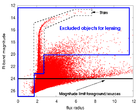
Figure 2: Magnitude vs. half-light radius plot of objects found by SExtractor in one particular field. Stars appear as almost vertical branch and can be separated from galaxies with high confidence. The solid and dashed box roughly encircles objects excluded for the lensing catalogue (Schirmer et al. 2003).

After the data reduction process, SExtractor (Bertin & Arnouts 1996) was used to compile a catalogue of source galaxy candidates needed for the cosmic shear analysis. For the rather conservative selection of source candidates, the final co-added science frames are first smoothed with a Gaussian kernel of $2.5$ pixel FHWM. One pixel corresponds to $0.\!\!^{\prime\prime}238$. A source candidate further needs to consist of at least $5$ contiguous pixels with a total flux greater than $1.5\,\sigma$ above the background noise level, and it has to possess a clearly defined quadrupole moment ($cl\neq 0$, analyseldac) and centroid. Stars and galaxies are distinguished in a magnitude vs. half-light radius plot of the selected objects (see Fig. 2 for an example). In this scatter plot, stars that are not too faint are clearly identified as a column of objects with roughly identical half-light radius $r_{\star}$. Objects with a half-light radius smaller than $r_{\star}$ are rejected as source candidates. An exception are objects in the faint part (fainter than $23.5\leavevmode\nobreak\ \rm mag$ in $R$-band) near this column.

As accurate measurements of galaxy shapes are the key in a weak lensing analysis, the quadrupole moments in the galaxy light profiles of the source candidates have to be corrected for PSF effects: atmospheric turbulence and instrumental effects also distort the galaxy images. This is done using the KSB method (Kaiser et al. 1995). A detailed description of the PSF correction procedure may be found in Erben et al. (2001), Heymans et al. (2006) or Hetterscheidt et al. (2006). The PSF fitting polynomial used is of order two or three.

In the estimators of the aperture statistics, every source galaxy is weighted with a statistical weight. This weight, $w_{i}$, is defined by the variance $\sigma^{2}_{\epsilon}$ in ellipticity of the $12$ nearest neighbours of a galaxy $i$ in the magnitude vs. half-light radius diagram: $w_{i}=1/(\sigma^{2}_{\epsilon}+\bar{\sigma}^{2})$, where $\bar{\sigma}^{2}=0.16$ is the variance of the unlensed galaxies. In the case that the PSF corrected ellipticity of a galaxy exceeds $\left|\epsilon\right|=1.0$ it automatically is attributed the weight zero and is hence not considered further in the analysis. Applying this cut removes rare outliers with unrealistic ellipticities, produced by the KSB technique. The final lensing catalogue is split into three magnitude bins BACK, BACK-II and BACK-III, see Table 1.

3.3 Selection of foreground objects

The actual foreground objects, of which the bias parameters are measured, are selected with the same SExtractor parameters as the galaxies candidates in the lensing catalogue. Galaxies are finally selected from this catalogue via a manually defined box in the magnitude/half-light radius diagram around the star branch.

Table 1: The table lists the limits of the magnitude bins, the total number of objects for all $52$ fields (deep, medium and shallow fields in GaBoDS), the mean redshift and the $1\sigma$-variance inside each bin.

Foreground object catalogue
sample	bin limits [mag]	#objects	$\langle z\rangle$
FORE-I	$19.5\leq R<21.0$	$6.5\times 10^{4}$	$0.34\pm 0.18$
FORE-II	$21.0\leq R<22.0$	$1.2\times 10^{5}$	$0.47\pm 0.22$
FORE-III	$22.0\leq R<23.0$	$2.5\times 10^{5}$	$0.62\pm 0.27$
Background source catalogue
sample	bin limits [mag]	#objects	$\langle z\rangle$
BACK	$21.5\leq R<24.0$	$6.2\times 10^{5}$	$0.67\pm 0.29$
BACK-II	$22.0\leq R<24.0$	$5.5\times 10^{5}$	$0.69\pm 0.28$
BACK-III	$23.0\leq R<24.0$	$3.5\times 10^{5}$	$0.74\pm 0.28$

In order to select for the bias analysis different mean redshifts of the (foreground) object catalogues, we subdivide the object catalogue into the three different $R$-band bins FORE-I, FORE-II and FORE-III as stated in Table 1.

Figure 3: Redshift distribution of the foreground and background galaxies as estimated from the photometric redshifts in the COMBO-17 fields A901, AXAF (CDFS) and S11 (dashed doted lines); the histograms are not normalised to unity. The solid lines are maximum-likelihood fits of Eq. (42) to the histograms.

3.4 Distribution in redshift of the galaxy samples

To estimate the redshift distribution of the galaxies – both foreground objects and background sources – we average the photometric redshift distribution in the different magnitude bins of the fields A901, AXAF and S11 (see Fig. 3). These three fields are contained in the deep part of the GaBoDS and were observed as part of the COMBO-17 survey (Wolf et al. 2004) in $17$ colours yielding quite accurate photometric redshifts with an uncertainty of $\delta z\approx 0.02\leavevmode\nobreak\ (1+z)$ for objects brighter than $R=23\leavevmode\nobreak\ \rm mag$. Less accurate but still available are photometric redshifts for objects with $23<R<24$. The photometric redshift distribution of the COMBO-17 galaxies is assumed to be representative for our whole catalogue.

High-redshift galaxies with $z>1.4$ are “missing” in the COMBO-17 sample because they were reassigned a redshift $z<1.4$. Recently, in Coe et al. (2006), the Hubble Ultra-Deep Field has been used to validate the photometric redshifts in COMBO-17. It has been found that the agreement is good for $R\lesssim 23.7$ and especially tight for $R<23$. We conclude, therefore, that we have got a reliable estimate of the redshift distribution in our samples.

For the source galaxies carrying the $M_{\rm ap}$-signal, the magnitude bin BACK is used throughout. As can be seen in Table 1, by varying only the lower limit, but keeping the upper limit of the magnitude bin fixed to $R=24\leavevmode\nobreak\ \rm mag$, one cannot shift the mean of the background redshift distribution to much higher values than $z\approx 0.7$; essentially, only the number of sources in the bin decreases. A large mean redshift of the source galaxies is desired to achieve a good lensing efficiency but more important is a large number of galaxies to achieve a good signal-to-noise ratio. Since we do not use objects fainter than $24\leavevmode\nobreak\ \rm mag$ in order to maintain good accuracy in the estimate for the redshift distribution of the background and to have a roughly homogeneous data set, the bin BACK for all three foreground bins FORE-I, FORE-II and FORE-III is the best choice.

The COMBO-17 sample used to estimate the redshift distribution in the galaxy sub-samples is relatively small. Clearly, it has features – large galaxy clusters or voids – which are not representative for the whole GaBoDS sample. For example, consider the peaks at low redshift in the foreground samples, Fig. 3. In order to have a smoother, more representative distribution we fit an empirical redshift distribution to the COMBO-17 histograms:

$$p(z)=\frac{1}{\Gamma(\frac{1+\alpha}{\beta})z_{0}}\left(\frac{z}{z_{0}}\right)^{\alpha}\,\exp{\left(-\left[\frac{z}{z_{0}}\right]^{\beta}\right)}\;.$$ (42)

The best-fits are shown in Fig. 3. They are used in the analysis further on instead of the COMBO-17 histograms. The best fit parameters are compiled in Table 2. These parameters are highly degenerate for which reason their statistical errors are not given in the table. However, statistical uncertainties of the mean redshift in the different samples and uncertainties of the galaxy bias parameters originating from uncertainties in $p(z)$ will be given in the following.

Clearly, the estimated redshift distributions still suffer from cosmic variance errors because the COMBO-17 survey area is with $\sim 0.75\,\rm deg^{2}$ relatively small. In order to get an estimate for the statistical uncertainties due to cosmic variance in the samples’ redshift distribution we use the widely applied Jackknife method: The photometric redshift distributions of merely two of the three fields are combined. With three ways of combining this yields overall $N=3$ Jackknife samples. To estimate the standard deviation of the mean redshift, $\bar{z}$, one computes from each Jackknife sample the mean redshift, $\bar{z}_{i}$. According to the Jackknife method the statistical $1\sigma$-error of the mean is then roughly:

$$\sigma^{2}(\bar{z})=\frac{N-1}{N}\sum_{i}(z_{i}-\bar{z})^{2}\;,$$ (43)

where $\bar{z}$ is the mean redshift obtained by combining all three COMBO-17 redshift distributions. The results for $\sigma(\bar{z})$ are listed in Table 2. As can be seen there the uncertainty of $\bar{z}$ ranges from $\sigma(\bar{z})/\bar{z}\approx 10\%$ to $\sigma(\bar{z})/\bar{z}\approx 2\%$ for FORE-I to BACK, respectively. This behaviour makes sense because the number of galaxies increases when going from the shallower to the deeper samples.

The problem of the calibration of redshift distributions for cosmic shear studies has recently been studied by van Waerbeke et al. (2006). They find a statistical uncertainty of $\sigma(\bar{z})=0.03-0.04$ for a $0.75\,\rm deg^{2}$ survey with mean $\bar{z}\sim 1$. This value is somewhat higher than our estimate.

The Jackknife samples can also be used to assess how the statistical uncertainty of the full $p(z)$’s translates into the inferred galaxy bias parameters. This problem will be addressed in Sect. 4.3.

Table 2: Best-fit parameters of the template redshift distribution, Eq. (42), to the COMBO-17 histograms. $\bar{z}$ is the mean of the template redshift distribution. The statistical errors of $\bar{z}$ are derived from the field-to-field variance in COMBO-17.

galaxy sample	$z_{0}$	$\alpha$	$\beta$	$\bar{z}$
FORE-I	0.534	0.509	3.173	$0.35\pm 0.03$
FORE-II	0.765	0.617	5.839	$0.47\pm 0.03$
FORE-III	0.945	0.830	5.103	$0.61\pm 0.02$
BACK	1.069	0.809	7.369	$0.68\pm 0.02$
BACK-II	1.072	0.988	7.655	$0.70\pm 0.02$
BACK-III	1.073	1.611	8.560	$0.77\pm 0.02$

4 Outline of the method

The approach to obtain the bias parameters from lensing adopted here proceeds in several steps:

1. estimating the binned correlators $\omega(\theta)$, $\langle\gamma_{\rm t}\rangle(\theta)$ and $\xi_{\pm}(\theta)$ in all individual survey fields,

2. numerical integration of the correlators to obtain $\langle N^{m}(\theta_{\rm ap})M_{\rm ap}^{n}(\theta_{\rm ap})\rangle$ for $m+n=2$ (E-modes and B-modes),

3. repetition of 1. and 2. with bootstrapped data sets to obtain statistical errors of the aperture statistics in the single fields,

4. combining the individual field measurements and evaluating the bias parameters as a function of aperture radius from the combined signal (includes calibration),

5. bootstrapping of the combined signal to estimate the error in the final signal and the covariances between the different bins.

A detailed account of these steps is given in the following.

4.1 Practical estimators for the correlators

The correlators are estimated by using

$$\omega\left(\theta\right) = \frac{DD}{RR}-2\frac{DR}{RR}+1,$$ (44)

$$\langle\gamma_{\rm t}\rangle\left(\theta\right) = \frac{\sum_{i,j}^{N_{\rm f},N_{\rm b}}\epsilon_{{\rm t},i}w_{i}\Delta_{ij}\left(\theta\right)}{\sum_{i,j}^{N_{\rm f},N_{\rm b}}w_{i}\Delta_{ij}\left(\theta\right)},$$ (45)

$$\xi_{\pm}\left(\theta\right) = \frac{\sum_{i,j}^{N_{\rm b}}w_{i}w_{j}\Delta_{ij}\left(\theta\right)\left(\epsilon_{{\rm t},i}\epsilon_{{\rm t},j}\pm\epsilon_{{\times},i}\epsilon_{{\times},j}\right)}{\sum_{i,j}^{N_{\rm b}}w_{i}w_{j}\Delta_{ij}\left(\theta\right)}\;,$$ (46)

where

$$\Delta_{ij}\left(\theta\right)\equiv\left\{\begin{array}[]{ll}1&{\rm for}\leavevmode\nobreak\ \theta\leq\left|\theta_{i}-\theta_{j}\right|<\theta+\delta\theta\\ 0&{\rm otherwise}\end{array}\right.\;.$$ (47)

The $w_{i}$ are statistical weights of the individual galaxies which are used to account for the fact that the values of the image ellipticities, $\epsilon_{i}$, of the galaxies do not have all the same accuracy. Ellipticities of fainter and smaller galaxies are determined with a lower accuracy than for larger and brighter galaxies. $N_{\rm f}$ and $N_{\rm b}$ are the number of foreground and background galaxies; $\epsilon_{{\rm t},i/j}$ and $\epsilon_{\times,i/j}$ are the tangential and cross ellipticity components relative to the line connecting the galaxy pair $i,j$.

The estimator of the spatial correlation $\omega(\theta)$ has been introduced by Landy & Szalay (1993). It requires to count the number of galaxy pairs with a separation between $\theta$ and $\theta+\delta\theta$, namely the number of pairs in the data (foreground galaxies), denoted by $DD$, the number of pairs in a random mock catalogue, $RR$, and the number of pairs that can be formed with one data galaxy and one mock data galaxy, $DR$. The random mock catalogue is computed by randomly placing the galaxies, taking into account the geometry of the data field, i.e. by avoiding outmasked regions. We make $40$ random galaxy catalogues and average the pair counts obtained for $DR$ and $RR$.

In an estimate of $\omega(\theta)$, Eq. (44), there is always an uncertainty about the mean galaxy density $\bar{n}$ which is the larger the smaller the area of the field under consideration. This introduces a bias known as the integral constraint (Groth & Peebles 1977), that systematically reduces the angular correlation, $\omega(\theta)\mapsto\omega(\theta)-C$, by a constant value $C>0$. As pointed out by Hoekstra et al. (2002) $\langle N^{2}\rangle$ is independent of the integral constraint when the aperture filter $u$ is, as in our analysis, compensated because

$$\int_{0}^{\infty}{\rm d}x\,x\,C\,T_{+}(x)=C\,\int_{0}^{\infty}{\rm d}x\,x\,T_{+}(x)=0\;.$$ (48)

Therefore the estimator bias $C$ does not make any contribution to $\langle N^{2}\rangle$ and does not need to be corrected. This nice feature makes the aperture statistics with a compensated filter a convenient tool to study galaxy clustering even outside a weak lensing context. We will briefly come back to this point in Sect. 5.

Concerning the estimator for mean tangential shear, $\langle\gamma_{\rm t}\rangle(\theta)$, all pairs of foreground and background galaxies within separation between $\theta$ and $\theta+\delta\theta$ have to be considered; $\epsilon_{{\rm t},i}$ is the tangential ellipticity component of the background galaxy with respect to the line connecting the foreground and background galaxy. Similarly, for $\xi_{\pm}(\theta)$ all pairs of background galaxies within some separation interval are considered.

For the GaBoDS analysis, we bin the three correlators into $800$ logarithmic bins spanning a range between $0.\!\!^{\prime\prime}05<\theta\leq 48^{\prime}$ (the diagonal of a single WFI field). In order to reduce the computation time for the correlations, a binary tree data structure as in Pen & Zhang (2003), Moore et al. (2001) or Jarvis et al. (2004) is used.

4.2 Aperture filter

To weight density fluctuations inside apertures we use a compensated polynomial filter (Hoekstra et al. 2002, 2001; Schneider et al. 1998)

$$u\left(x\right)=\frac{9}{\pi}\left(1-x^{2}\right)\left(\frac{1}{3}-x^{2}\right)\,H(1-x)\;,$$ (49)

which by definition vanishes for $x\geq 1$; $H(x)$ denotes the Heaviside step function. The filter has the effect that only matter or galaxy number density fluctuations from a small range of angular scales contribute to the $N$- or $M_{\rm ap}$-signal; it acts as a narrow-band filter for the angular modes with highest sensitivity to $\ell_{\rm c}\sim 4.25/\theta_{\rm ap}\approx 0.68\times 2\pi/\theta_{\rm ap}$. Apertures with radius $\theta_{\rm ap}$ therefore effectively probe a comoving physical scale of $f_{\rm K}(\bar{w})\,\theta_{\rm ap}/0.68$, if $\bar{w}$ is the median comoving radial distance of the galaxy sample under examination.

All auxiliary functions (40)-(41), which are required for transforming the correlators, vanish outside the interval $x\in\left[0,2\right]$ due to the finite support of $u$. This reduces the transformation integrals (2.3)-(39) to a finite integration range $[0,2\theta_{\rm ap}]$. Therefore, with square $30^{\prime}\times 30^{\prime}$ WFI fields we are able to estimate the aperture moments out to about $\frac{1}{2}\sqrt{2}\,30^{\prime}\approx 21^{\prime}$.

4.3 Calibration of bias parameters

Figure 4: Left: The two figures show the scale-dependence of the calibration factors $f_{1/2}$, for sample FORE-I only, for three different fiducial cosmologies; SCDM (dotted): $\Omega_{\rm m}=1.0$, $\Omega_{\Lambda}=0$; $\Lambda\rm CDM$ (solid): $\Omega_{\rm m}=0.3$, $\Omega_{\Lambda}=0.7$; OCDM (dashed): $\Omega_{\rm m}=0.3$, $\Omega_{\Lambda}=0$. Right: These plots were obtained by averaging $f_{1/2}$ over a range of aperture radii, $1^{\prime}\leq\theta_{\rm ap}<60^{\prime}$, assuming different fiducial cosmologies. For all cosmologies, $\Omega_{\rm m}$ is the only free parameter. The others are: $\Omega_{\Lambda}=1-\Omega_{\rm m}$, $\Gamma=\Omega_{\rm m}h$, $\sigma_{8}=0.41\,\Omega_{\rm m}^{-0.56}$ and $h=0.7$. The average values for $f_{1/2}$ in this figure are divided by $f_{1/2}(\Omega_{\rm m}=0.3)$, the here adopted calibration. For $p_{\rm f}(z)$, we have FORE-I (solid), FORE-II (dashed) and FORE-III (dotted); $p_{\rm b}(z)$ is as in BACK.

To summarise, the aperture mass $M_{\rm ap}$, Eq. (10), is proportional to the (weighted) projected total matter density contrast $\delta_{\rm m}$, whereas the aperture number count $N$, Eq. (14), is proportional to the number density contrast of the galaxy distribution $\delta_{\rm g}$. Both aperture measures are defined on some scale by the filter function $u$ and the aperture size $\theta_{\rm ap}$. This is exactly what we need to study the biasing of the galaxy distribution with respect to the matter distribution, as has been pointed out by Schneider (1998) and van Waerbeke (1998). Therefore, we can define biasing parameters in analogy to Eqs. (2) (Hoekstra et al. 2002)

$$b\left(\theta_{\rm ap}\right) = f_{1}\left(\theta_{\rm ap}\right)\sqrt{\frac{\langle N^{2}\left(\theta_{\rm ap}\right)\rangle}{\langle M^{2}_{\rm ap}\left(\theta_{\rm ap}\right)\rangle}}\;,$$ (50)

$$r\left(\theta_{\rm ap}\right) = f_{2}\left(\theta_{\rm ap}\right)\frac{\langle N\left(\theta_{\rm ap}\right)M_{\rm ap}\left(\theta_{\rm ap}\right)\rangle}{\sqrt{\langle N^{2}\left(\theta_{\rm ap}\right)\rangle\langle M^{2}_{\rm ap}\left(\theta_{\rm ap}\right)\rangle}}\;.$$

The three-dimensional number density that $N$ is sensitive to covers in general not the same volume that is probed by $M_{\rm ap}$ ($p_{\rm f}(w)$ versus $\overline{W}(w)$). Naively identifying $N$ with the galaxy number density contrast, $\delta_{\rm g}$, and $M_{\rm ap}$ with the matter density contrast, $\delta_{\rm m}$ therefore gives the wrong bias parameters. This $N/M_{\rm ap}$-mismatch in sensitivity to density fluctuations at the same radial distance thus requires to make a correction of the bias parameters which is done by means of the calibration factors $f_{1/2}$.

According to Hoekstra et al. (2002), the calibration factors have to be calculated based on some theoretical $P_{\rm m}(k,w)$ by means of

$$f_{1}\left(\theta_{\rm ap}\right) = \left.\sqrt{\frac{\langle M^{2}_{\rm ap}\left(\theta_{\rm ap}\right)\rangle}{\langle N^{2}\left(\theta_{\rm ap}\right)\rangle}}\right|_{r=b=1}\;,$$ (51)

$$f_{2}\left(\theta_{\rm ap}\right) = \left.\frac{\sqrt{\langle N^{2}\left(\theta_{\rm ap}\right)\rangle\langle M^{2}_{\rm ap}\left(\theta_{\rm ap}\right)\rangle}}{\langle N\left(\theta_{\rm ap}\right)M_{\rm ap}\left(\theta_{\rm ap}\right)\rangle}\right|_{r=b=1}\;,$$

where $\langle N^{n}(\theta_{\rm ap})M^{m}_{\rm ap}(\theta_{\rm ap})\rangle$, $n+m=2$, in these equations have to be evaluated by Eqs. (18)-(20) and (26)-(28), specifically for the redshift distributions of foreground, $p_{\rm f}(z)$, and background galaxies, $p_{\rm b}(z)$, in the data and for a fiducial cosmological model assuming that galaxies are not biased with respect to the dark matter, i.e. $b(k,w)=r(k,w)=1$.

Importantly, it turns out (van Waerbeke 1998) that the calibration factors $f_{1}$ and $f_{2}$ vary only slightly, mostly on scales below $\theta_{\rm ap}\lesssim 5^{\prime}$, for realistic aperture radii $\theta_{\rm ap}$ within a fixed fiducial cosmological model. This is strictly true if the dark matter power spectrum can be described by a power law, or – since we are, for a fixed aperture radius, sensitive to only a very localised range in $\ell$-space due to the adopted aperture filter – if the power spectrum is approximately a power law over the selected range in Fourier space.

For examples, see Fig. 4 (upper left and bottom left) where $f_{1/2}$ are plotted for three fiducial cosmological models assuming the redshift distribution of FORE-I and BACK. The calibration factors show very little dependence on $\theta_{\rm ap}$. Hence, a scale-dependence of the uncalibrated measurements immediately indicates a real scale-dependence in the bias parameter without fixing the fiducial cosmology! Moreover, it means that the calibration factors can be worked out for the linear or quasi-linear regime which is understood much better than the non-linear regime. Still, when calibrating our measurements we also take into account the dependence on scale.

We calculated the calibration factors $f_{1/2}$ for a range of spatially flat fiducial cosmologies, $\Omega_{\rm m}+\Omega_{\Lambda}=1$, using the redshift distribution in our data set (right column in Fig. 4), assuming constraints on $\sigma_{8}\propto\Omega_{\rm m}^{-0.56}$ from cluster abundances (White et al. 1993) and the shape parameter $\Gamma=\Omega_{\rm m}h$ for a negligible baryon density $\Omega_{\rm b}\approx 0$ (Efstathiou et al. 1992). The relation between $\sigma_{8}$ and $\Omega_{\rm m}$ is scaled such that $\sigma_{8}=0.8$ corresponds to $\Omega_{\rm m}=0.3$. This value of $\sigma_{8}$ for the power spectrum normalisation is suggested by the GaBoDS data (Hetterscheidt et al. 2006). Note that the value of $\sigma_{8}$, like for example $\sigma_{8}=0.9$ instead of $\sigma_{8}=0.8$, has virtually no impact on $f_{1/2}$ and, therefore, on the measured linear stochastic bias.

Predicting the power spectra, $P_{\kappa}$, $P_{\kappa\rm n}$ and $P_{\rm n}$, requires a model for the redshift evolution of the 3D power spectrum $P_{\rm m}(k,w)$. We use the standard prescription of linear structure growth and the Peacock and Dodds (1996) prescription for the evolution in the non-linear regime. A more recent and more accurate description of the non-linear power spectrum is given by Smith et al. (2003). Although Smith et al. predict in general more clustering on smaller scales than Peacock & Dodds, we found in a comparison between both methods only little difference for $f_{1/2}$.

It becomes clear from Fig. 4 that particularly the interpretation of the bias factor, $b$ (calibration $f_{1}$), depends on $\Omega_{\rm m}$. For the final calibration of the GaBoDS measurements we assume as fiducial cosmological model $\Omega_{\rm m}=0.3,\,\Omega_{\Lambda}=0.7,\,\sigma_{8}=0.8,\,\Gamma=0.21,\,h=0.7$.

The calibration procedure outlined here works because correlations between fluctuations seen in $N$ and $M_{\rm ap}$ stemming from different redshifts quickly vanish with increasing mutual redshift difference. This allows us to correct for a mismatch in the cosmic volumes seen by $N$ and $M_{\rm ap}$ – for the price of making assumptions about the fiducial cosmology, though. In fact, the mismatch is quantified by the factor $1/f_{2}$ which is the correlation factor of the (projected) fluctuations seen in $N$ and those seen in $M_{\rm ap}$ assuming that galaxies perfectly trace mass. If this factor is exactly $1/f_{2}=1$ for all scales, we will immediately know that $N$ and $M_{\rm ap}$ probe exactly the same cosmic volume giving equal weight to all radial distances. For our samples and fiducial cosmology, we find $1/f_{2}=0.95,0.95,0.84$ (FORE-I to FORE-III) indicating that the mismatch is relatively small.

4.4 Uncertainties in the calibration factors

Concerning the statistical errors of the calibrated galaxy bias parameters it has to be considered that the redshift distributions of the galaxy samples are not exactly known (Sect. 3.4). Since the calibration just involves a rescaling by $f_{1/2}$, any relative error in $f_{1/2}$ results in an equal relative error in $b(\theta_{\rm ap})$ and $r(\theta_{\rm ap})$. To estimate the relative error in $f_{1/2}$, $\sigma(f_{1/2})/f_{1/2}$, we use again the three Jackknife samples of the redshift distributions that have already been used in Sect. 3.4. Every histogram of photometric redshifts of every Jackknife sample is fitted by the template distribution (42). Then, for our fiducial cosmology and for every galaxy sample, we compute $f_{1/2}$ for each Jackknife $p(z)$-template. Thus, for any sample we obtain a triplet of values for the bias calibration. Then, as in Sect. 3.4, the variance between the different $f_{1/2}$’s is used as estimate of the $1\sigma$-error of the calibration parameters. Following this procedure, we find that the statistical uncertainty in the calibration due to cosmic variance uncertainties in $p(z)$ is (FORE-I to FORE-III): $\sigma(f_{1})/f_{1}=16\%,4\%,3\%$ and $\sigma(f_{2})/f_{2}=4\%,2\%,8\%$, respectively. Thus, the relative error is roughly $\sigma(f_{1/2})/f_{1/2}\lesssim 7\%$, except for $f_{1}$ of FORE-I where we have $\sigma(f_{1})/f_{1}=16\%$. We expect similar relative errors for other cosmological models.

Another issue is the impact of uncertainties in the fiducial cosmological model on the calibration parameters, which in return influences the inferred galaxy bias. Using Fig. 4 we estimate the relative change in $f_{1/2}$ with $\sim\pm 7\%$ ($f_{1}$) and $\sim\pm 2\%$ ($f_{2}$) when changing $\Omega_{\rm m}=0.3$ by $\pm 10\%$. Therefore, having $\Omega_{\rm m}$ wrong by about $\pm 10\%$ introduces a systematic error into the bias parameters which is about $\pm 7\%$ for $b$ and about $\pm 2\%$ for $r$.

4.5 Redshift and scale resolution

Figure 5: The bias parameters estimated in this paper are averages over some redshift range, plotted here as a function of aperture radius; plotted is the mean, $z_{\rm c}$, (solid line) and variance, $\sigma_{z}$, (shaded area) of the weight functions $h_{1/3}(z,\theta_{\rm ap})$ for each foreground sample. Mean and variance do not change significantly with aperture radius, $\theta_{\rm ap}$. The average of $z_{\rm c}$ and $\sigma_{z}$ over all radii, $z_{\rm c}\pm\sigma_{z}$, is indicated in each panel. Left column: weight function for the bias factor, $h_{1}$. Right column: weight function for the correlation parameter, $h_{3}$.

The bias parameters obtained by Eqs. (50) are in general averages of the true bias parameters $b(k,w)$ and $r(k,w)$, Eqs. (31), namely averaged over some scale $k$ and comoving distance (redshift) $w$. In other words, the method applied here has a limited resolution in redshift and scale. This is due to two reasons: 1. the sample of foreground galaxies is usually not peaked at one particular redshift but smeared out over some range, and 2. lensing is, with varying response, sensitive to the whole matter distribution between a source galaxy and the observer. According to Hoekstra et al. (2002), the observed weighted averages, $\langle b^{2}\rangle$ and $\langle r\rangle$, when using the polynomial aperture filter, Eq. (49), are approximately

$$\langle b^{2}\rangle(\theta_{\rm ap}) \approx \frac{\int_{0}^{w_{h}}{\rm d}w\,h_{1}(w,\theta_{\rm ap})\,b^{2}(\frac{4.25}{\theta_{\rm ap}f_{\rm K}(w)},w)}{\int_{0}^{w_{h}}{\rm d}w\,h_{1}(w,\theta_{\rm ap})}\;,$$ (52)

$$\langle r\rangle(\theta_{\rm ap}) \approx \frac{\int_{0}^{w_{h}}{\rm d}w\,h_{3}(w,\theta_{\rm ap})\,r(\frac{4.25}{\theta_{\rm ap}f_{\rm K}(w)},w)}{\int_{0}^{w_{h}}{\rm d}w\,h_{3}(w,\theta_{\rm ap})}\;,$$ (53)

where the following weight functions have been introduced

$$h_{1}(w,\theta_{\rm ap}) = \left(\frac{p_{\rm f}(w)}{f_{\rm K}(w)}\right)^{2}\,P_{\rm filter}(w,\theta_{\rm ap})\;,$$ (54)

$$h_{3}(w,\theta_{\rm ap}) = \frac{p_{\rm f}(w)\overline{W}(w)}{[f_{\rm K}(w)]^{2}}\,P_{\rm filter}(w,\theta_{\rm ap})\;,$$ (55)

with

$$P_{\rm filter}(w,\theta_{\rm ap})=$$

$$2\pi\int_{0}^{\infty}{\rm d}\ell\,\ell\,P_{\rm m}\left(\frac{\ell}{f_{\rm K}(w)\theta_{\rm ap}},w\right)[I(\ell\theta_{\rm ap})]^{2}\;.$$ (56)

Note that in general the central redshift and the width of the weights depends on the aperture radius $\theta_{\rm ap}$.

We calculated the functions $h_{1}(z,\theta_{\rm ap})$ and $h_{3}(z,\theta_{\rm ap})$ for accessible aperture radii for the redshift distributions in our galaxy samples and for the adopted fiducial cosmological model. As typical redshift at which $b$ and $r$ are measured we take – for every aperture radius $\theta_{\rm ap}$ – the mean, $z_{\rm c}$, of the kernels $h_{1}$ and $h_{3}$, and as a measure for the redshift range over which the bias parameters are averaged we take the width, $\sigma_{z}$, of the kernels $h_{1}$ and $h_{3}$ (see Fig. 5). With $z_{\rm c}$ being the typical redshift, the typical spatial scale corresponds to $k_{\rm c}=\frac{4.25}{\theta_{\rm ap}f_{\rm K}(w(z_{\rm c}))}$ (3D Fourier mode) or $R_{\rm c}=2\pi/k_{\rm c}\approx 1.48\,\theta_{\rm ap}f_{\rm K}(w(z_{\rm c}))$; the redshift resolution achieved is roughly $\sigma_{z}$ which also adds an uncertainty to the effective scale probed, $\sigma_{R}$, with a relative error of about $\sigma_{R}/R_{\rm c}=\sigma_{z}/z_{\rm c}$.

Figure 6: The aperture number count dispersions, as measured in GaBoDS, for FORE-I (filled boxes), FORE-II (open stars) and FORE-III (open crosses). The $1\sigma$ error bars have the size of the data points. Upper panel: comparison to $\Lambda\rm CDM$ predictions assuming unbiased galaxies, upper to lower line: FORE-I (solid), FORE-II (dashed) and FORE-III (dotted). Lower panel: power laws give excellent descriptions of the measurements. The dotted-dashed line denotes $\langle N^{2}\rangle$ as measured by Hoekstra et al. (2002) ($A_{\omega}=0.115$, $\delta=0.7$).

4.6 Combining measurements from different fields

Bootstrapping I.

The whole data set taken into account for the analysis consists of $N_{\rm p}=52$ fields. For each field, we compute the two-point correlation estimates as in Sect. 4.1 and transform them according to the integrals Eqs. (2.3)-(39) to the $2^{\rm nd}$-order aperture statistics. For every individual field, $j$, we make $200$ bootstrap samples of the foreground and background object catalogues to estimate the statistical error of the measurements

$$x_{i}^{(j)}\!\!\in\!\!\{\langle N^{2}(\theta_{{\rm ap},i})\rangle,\langle N(\theta_{{\rm ap},i})M_{{\rm ap}}(\theta_{{\rm ap},i})\rangle,\langle M^{2}_{{\rm ap}}(\theta_{{\rm ap},i})\rangle\}\;,$$ (57)

for the various aperture radii $\theta_{{\rm ap},i}$. The aperture moments $x_{i}^{(j)}$ from all fields are combined to one final result, $\bar{x}_{i}$, by the weighted average

$$\bar{x}_{i}=\frac{\sum_{j=1}^{N_{p}}x_{i}^{(j)}\,w_{ij}}{\sum_{j=1}^{N_{p}}\,w_{ij}}\;.$$ (58)

As weight we use the reciprocal bootstrapping variance of $x_{i}^{(j)}$ in the individual fields, $w_{ij}=1/\sigma^{2}(x_{i}^{(j)})$. This weighting scheme yields the minimum-variance estimate of the average $\bar{x}_{i}$.

Bootstrapping II.

In a second bootstrapping stage, we randomly draw fields from the set of $52$ GaBoDS fields (with putting back) and calculate a combined signal according to Eq. (58) for this bootstrap sample. We repeat this procedure $2000$ times. This estimates the PDF of statistical errors in the combined signal including cosmic variance and accounting for the adopted weighting scheme. In addition to the combined signal of the aperture moments, we use this technique to also estimate the PDF of statistical errors of the bias parameters $r(\theta_{\rm ap})$ and $b(\theta_{\rm ap})$, Eqs. (50), which are computed from the weighted average of the aperture statistics. Based on the bootstrap samples we obtain the median, (asymmetric) $68\%$ confidence intervals about the median and covariances of the errors for the final results.

5 Results

5.1 Aperture statistics

Figure 7: Top row panels and lower left panel: cross-correlation between aperture mass and aperture number count for the three different foreground samples FORE-I (solid boxes), FORE-II (open stars) and FORE-III (open crosses). The panels are subdivided; the lower panel shows the B-mode, upper panel is the E-mode of $\langle NM_{\rm ap}\rangle$. The curves are $\Lambda\rm CDM$ predictions assuming unbiased galaxies. Lower right: aperture mass dispersion, lower and upper panel are B-mode and E-mode, respectively. The solid line is a $\Lambda\rm CDM$ prediction. The solid lines in the B-mode panel are the E-mode prediction with positive and negative sign, which have been inserted for comparison.

The combined measurements for $\langle N^{2}\rangle$, $\langle NM_{\rm ap}\rangle$ and $\langle M^{2}_{\rm ap}\rangle$ can be found in Fig. 6 and Fig. 7.

Galaxy clustering.

Traditionally, galaxy clustering is studied using the angular correlation function $\omega(\theta)$. For a comparison of our results for the two-point statistics of galaxy clustering with the literature it would be convenient to have $\omega(\theta)$ cleaned from the integral constraint. Already from early studies on galaxy clustering (e.g. Davis & Peebles 1983) up to recent studies (Norberg et al. 2001; Zehavi et al. 2002) it is known that $\omega(\theta)$ is close to a power law over a wide range, thus

$$\omega(\theta)=A_{\omega}\,\left(\frac{\theta}{1^{\prime}}\right)^{-\delta}\;,$$ (59)

where $A_{\omega}$ and $\delta$ are the clustering amplitude at $1^{\prime}$ and the clustering power law index, respectively. Assuming this power law, we can calculate the aperture number count dispersion for our polynomial aperture filter:

$$\langle N^{2}\rangle(\theta)=\int_{0}^{2}{\rm d}x\,x\,\omega(\theta\,x)\,T_{+}(x)=f(\delta)\,A_{\omega}\,\left(\frac{\theta}{1^{\prime}}\right)^{-\delta},$$ (60)

with $f(\delta)$ being defined in (66). Therefore, if $\omega(\theta)$ is a power law, the aperture number count dispersion is also a power law with the same slope but different amplitude. Since $\langle N^{2}\rangle$ is free of the integral constraint, we can recover $\omega(\theta)$ from $\langle N^{2}\rangle$ by fitting a power law and rescaling the best-fit amplitude by means of the function (66). For determining the statistical uncertainties of $A_{\omega}$, however, we have to take into account that it is not only a function of the amplitude of $\langle N^{2}\rangle$ but also a function of the slope $\delta$.

We performed fits of (60) to the data taking into account the covariances of $\langle N^{2}\rangle$ obtained by bootstrapping, see Fig. 6. What is concluded for our foreground samples is summarised in Table 3.

Table 3: Amplitude and slope of the angular correlation, $\omega(\theta)=A_{\omega}\,(\theta/1^{\prime})^{-\delta}$, in our foreground galaxy samples as inferred from $\langle N^{2}\rangle(\theta_{\rm ap})$; $\chi^{2}/n$ denotes the reduced $\chi^{2}$ ($n=12-2$) of the maximum-likelihood fit.

galaxy sample	$A_{\omega}$	$\delta$	$\chi^{2}/n$
FORE-I	$0.086\pm 0.006$	$0.89\pm 0.05$	$1.0$
FORE-II	$0.044\pm 0.003$	$0.99\pm 0.04$	$0.6$
FORE-III	$0.026\pm 0.002$	$0.90\pm 0.04$	$1.8$

The angular correlation of the galaxies in FORE-I – a sample roughly comparable to the foreground sample of Hoekstra et al. (2002) – has a slope slightly steeper than what is found in the sample of Hoekstra et al. (there $\delta=0.7$ and $A_{\omega}=0.115$) and is smaller in amplitude for aperture radii larger than $\theta_{\rm ap}\approx 3^{\prime}$. This discrepancy in $A_{\omega}$ and $\delta$ is not as drastic as it may seem if one takes into account that the errors of $A_{\omega}$ and $\delta$ are anti-correlated: a smaller $A_{\omega}$ results in a steeper $\delta$. Another issue that may play a role in this context is the fact that Hoekstra et al. use a different filter, $R_{c}$, which is somewhat different from our $R$-band filter. All in all we think that the measurement of $\omega(\theta)$ for FORE-I is consistent with the measurement of Hoekstra et al.

Compared to the $\Lambda\rm CDM$ prediction of $\langle N^{2}\rangle$ for unbiased galaxies, which trace the dark matter distribution, our measurements are clearly different, namely exceeding the dark matter expectation on scales smaller than $\theta_{\rm ap}\approx 5^{\prime}$, and falling slightly below the prediction for the largest aperture radii. This already suggests a scale-dependence of the bias factor.

Dark matter clustering.

Figure 8: The measured two-point cosmic shear auto correlation in terms of $\xi_{\pm}=\langle\gamma_{\rm t}\gamma_{\rm t}\rangle\pm\langle\gamma_{\times}\gamma_{\times}\rangle$. The dotted curve is a $\Lambda\rm CDM$ prediction based on $p_{\rm b}(w)$ as in the sample BACK.

Figure 9: Plot of the measured mean tangential shear, $\langle\gamma_{t}\rangle$, about galaxies in our foreground samples FORE-I (filled boxes), FORE-II (open stars) and FORE-III (open crosses) as a function of angular separation. The lines are $\Lambda\rm CDM$ predictions assuming unbiased galaxies, $p_{\rm f}(w)$ and $p_{\rm b}(w)$ as estimated in our samples: for FORE-I (solid), FORE-II (dashed) and FORE-III (dotted).

The clustering of the total matter content as derived from the ellipticities of the background galaxies is expressed by the dispersion of the aperture mass, Fig. 7. We calculated this quantity for a range of different aperture radii from the cosmic shear two-point correlators, $\xi_{\pm}$, which are shown in Fig. 8 (rebinned for that plot).

In all figures, the prediction for the adopted fiducial cosmological model and the estimated redshift distributions in our galaxy samples is plotted. We conclude that this prediction is in good agreement with our measurements. Therefore the fiducial cosmology taken for the bias parameter calibration seems to be reasonable.

Judging from the B-modes, $\langle M_{\times}^{2}\rangle$, in Fig. 7, which serve as an indicator for systematics in the PSF correction, the PSF correction is ok. Over the whole range of aperture radii considered the B-modes are consistent with zero, maybe with a minor exception at about $\theta_{\rm ap}\approx 3^{\prime}$. See Hetterscheidt et al. (2006) for a detailed discussion on this issue.

Correlation between galaxy and matter distribution.

The cross-correlation between the $N$-maps and the $M_{\rm ap}$-maps is plotted in Fig. 7. Apart from $\theta_{\rm ap}\approx 3^{\prime}$ in FORE-II the B-modes of the signal are all consistent with zero. The cross-correlation has been worked out on the basis of the mean tangential shear about galaxies in the foreground samples. Results for the galaxy-galaxy lensing signal are depicted in Fig. 9.

The data points (E-mode) on intermediate scales are below the theoretical prediction for $\langle NM_{\rm ap}\rangle$ based on an unbiased galaxy population. This again indicates that either the bias factor or the correlation parameter or both differ from unity, hinting towards a population of galaxies that does not perfectly trace the (dark) matter distribution.

5.2 Galaxy bias parameters

Figure 10: The linear stochastic bias parameters of galaxies in the samples FORE-I, FORE-II and FORE-III (left to right column); the bias factor, $b$, is upper, the correlation parameter, $r$, is in the lower row. The parameters have been calibrated assuming $\Omega_{\rm m}=0.3$ and $\Omega_{\Lambda}=0.7$ (see Fig. 4). The effective comoving scale is based on the aperture radius and the mean redshift of the weight functions $h_{1/3}$, Fig. 5. The bias parameters for a particular aperture radius are averages over different physical scales and redshifts (Sect. 4.5). The shaded area denotes the average bias factor or correlation factor over all aperture radii between $\theta_{\rm ap}=2^{\prime}\ldots 19^{\prime}$; the maximum-likelihood of this average and its statistical uncertainty are shown in numbers inside the panels.

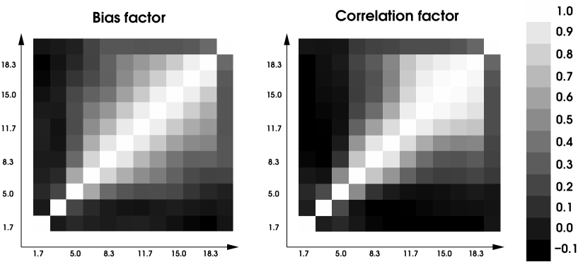
Figure 11: Correlations of the statistical errors of the bias factor (left panel) and correlation factor (right panel) of galaxy sample FORE-II as inferred from the bootstrap samples; the correlation matrices of samples FORE-I and FORE-III are virtually identical. The colour of one pixel in an intensity map denotes the correlation between the errors belonging to the two bins defined by the x- and y-axis; the key of the intensity map is on the right side. The numbers attached to the axis denote the aperture radii in arcmin corresponding to the individual bins in Fig. 10.

The final result of our work is displayed in Fig. 10. The bias parameters calculated from the aperture statistics, Eqs. (50), have been calibrated, and the aperture radii have been converted into a typical physical scale, $R$, based on the mean redshift of the range over which the parameters are averaged. As this redshift range stretches over about $40\%-50\%$ ($1\sigma$) of the mean redshift (see Fig. 5), there is a relative uncertainty attached to the physical range, $R$, which is of the same order; for instance for $R=6\,h^{-1}\rm Mpc$ we have as resolution for the effective scale $\sigma_{R}=3\,h^{-1}\rm Mpc$ (see Sect. 4.5).

Over the range of (comoving) physical scales investigated, below about $R\lesssim 10\,h^{-1}\rm Mpc$, the bias factor stays more or less constant, rising towards smaller and possibly also larger scales with a valley on intermediate scales, where $b$ becomes slightly inconsistent with $b=1$ at a $68\%$ confidence level; this implies a scale-dependence of the bias factor. As absolute minimum we obtain $b_{\rm min}=0.78\pm 0.10,0.74\pm 0.10,0.78\pm 0.10$ at roughly $\theta_{\rm ap}\approx 10^{\prime}$. The position of the minimum is not well defined, however, due its width. In order to get an average value for the bias factor, we make a maximum likelihood fit assuming a constant bias over the range $2^{\prime}\leq\theta_{\rm ap}\leq 19^{\prime}$ while taking into account the covariance between the errors, as estimated from the bootstrap samples, shown in Fig. 11. This fit yields: $\bar{b}=0.81\pm 0.11,0.79\pm 0.10,0.81\pm 0.11$ for FORE-I, FORE-II and FORE-III, respectively. Therefore, over the selected range of scales, galaxies are anti-biased, i.e. less clustered than the dark matter.

The correlation factor, $r$, has a larger relative uncertainty than the bias factor, $b$, since it is based on two lensing quantities, $\langle NM_{\rm ap}\rangle$ and $\langle M_{\rm ap}^{2}\rangle$, which are generally noisier than $\langle N^{2}\rangle$. Broadly speaking, the correlation of the galaxies to the (dark) matter distribution is relatively high. A scale-dependence of the correlation factor is hard to determine due to the large uncertainties and the high correlation of neighbouring bins; it may be present in the sample FORE-I. Averaging the correlation factor over $2^{\prime}\leq\theta_{\rm ap}\leq 19^{\prime}$ yields $\bar{r}=0.61\pm 0.16,0.64\pm 0.16,0.58\pm 0.19$ (FORE-I to FORE-III) which reflects both the high correlation and the unfortunately still large error bars. Obviously, a much larger survey area is required to obtain better constraints. We are going to discuss our results in the following section.

6 Discussion and conclusions

Observationally, the galaxy-dark matter bias can be probed by means of various methods (see introduction). Gravitational lensing provides a promising new method in this respect. It is special because it allows for the first time to map the total matter content (mainly dark matter) with a minimum of assumptions and independent of the galaxy distribution. Such a map can be compared to the distribution of galaxies, or particular types of galaxies, in order to investigate the galaxy bias. In particular, correlations between galaxy and dark matter density become directly visible. For working out the galaxy-dark matter bias, older methods rely on assumptions regarding the growth of dark matter density perturbations, the peculiar velocities of galaxies and their correlation to the dark matter density. Moreover, they often only allow one to measure the bias on large (linear) scales, $\gtrsim 8\,h^{-1}\rm Mpc$, whereas the non-linear regime is also accessible with lensing. However, gravitational lensing has the disadvantage that it is not equally sensitive at all redshifts. The cosmic shear signal is most sensitive to matter fluctuations roughly half-way between $z=0$ and the mean redshift of the background. This defines a natural best-suited regime for the method at a redshift of about $z\approx 0.5$, often even slightly lower, considering the depth of current galaxy surveys. It is expected that the most sensitive regime will be shifted towards higher redshifts by future space-based lensing surveys. Furthermore, lensing observables are quite noisy so that large survey areas are required for a good signal-to-noise. Impressively large surveys with instruments such as the CFHT (CFHT-Legacy-Survey, CFHTLS), the VST (Kilo-Square-Degree-Survey, KIDS), Pan-STARRS, or SNAP are either ongoing or about to start within the next years, providing us with plenty of high signal-to-noise information on dark matter and galaxy clustering.

In this paper, we employed aperture statistics to quantify the relation between the dark matter and galaxy density. We tested the evaluation software against Monte Carlo simulated WFI fields, assuming an unbiased galaxy population, and found that the software is working to at least a few percent accuracy (Simon 2005). The data used is the GaBoDS with restriction to galaxies brighter than $24\,\rm mag$ in the $R$-band; this allowed us to estimate the redshift distribution of the galaxies on the basis of three COMBO-17 fields (A901, AXAF/CDFS and S11) for which photometric redshifts in $0\leq z\lesssim 1.4$ are available. For all the other fields, only $R$-band magnitudes can be used to select galaxies. For this selection, we defined foreground galaxy samples by choosing galaxies from three $R$-band magnitude bins that have increasingly fainter median magnitudes. The sample FORE-I is comparable to the foreground selection in Hoekstra et al. (2002) who applied the same technique as we are using here. By means of the photometric redshifts of the COMBO-17 fields we can translate a GaBoDS R-band magnitude interval into a redshift distribution. The fainter the bin, the broader the redshift distribution, while the mean redshift moves to larger values. Therefore, only FORE-I has a rather sharp peak in redshift, while FORE-III stretches between redshifts of about $z=0.1$ and $z\approx 0.9$. Hence, FORE-II and FORE-III are averages over a relatively wide range of redshifts. In order to get narrower distributions in redshifts with the aim to reconstruct the redshift evolution of biasing, multi-colour lensing surveys are required. Cosmic variance is the main uncertainty in the estimated redshift distribution. Based on the field-to-field variance of the photometric redshift distributions we estimate that this uncertainty translates into a $1\sigma$-uncertainty of the bias parameters of $\sim 7\%$, except for the bias factor, $b$, in FORE-I which has $\sim 16\%$.

The B-mode of the aperture statistics $\langle NM_{\rm ap}\rangle$ and $\langle M^{2}_{\rm ap}\rangle$ are used as an indicator for systematics in the PSF-corrected shapes of the background galaxies (Fig. 7); they cannot be produced by gravitational lensing and should therefore be pure noise. We find that the B-modes are consistent with zero, maybe leaving a small question mark at $\theta_{\rm ap}\approx 3^{\prime}$. Note that, at least in principle, physical effects like intrinsic alignments of the source galaxies can be a source of B-modes in $\langle M^{2}_{\rm ap}\rangle$ (on small scales), so that vanishing B-modes are not the ultimate indicators of PSF systematics. For $\langle NM_{\rm ap}\rangle$, however, the only possible source of B-modes is a violation of a statistical parity-invariance (Schneider 2003). Therefore, $\langle NM_{\rm ap}\rangle$ should always be B-mode free which is clearly the case in our data.

The fit of a theoretical $\langle M^{2}_{\rm ap}\rangle$ constructed from our fiducial cosmology and redshift distribution of source galaxies to the measured $\langle M_{\rm ap}^{2}\rangle$ is an important test for the calibration of the bias parameter; $\langle M^{2}_{\rm ap}\rangle$ is independent of the galaxy bias. Our data points are consistent with the fiducial cosmological model and, therefore, we accept the fiducial cosmological model and the estimated redshift distributions as sufficiently accurate for our purposes. For fiducial cosmological models different from ours (but still flat, $\Omega_{\rm m}+\Omega_{\Lambda}=1$, with negligible baryon density, $\Gamma=\Omega_{\rm m}h$, and $h=0.7$, and $\sigma_{8}\propto\Omega_{\rm m}^{-0.56}$) the calibrated bias parameters in Fig. 10 may be scaled up or down using Fig. 4. In a related paper (Hetterscheidt et al. 2006), we discuss in much more detail issues concerning the creation of source galaxy catalogues and their data quality, and we determine constraints on cosmological parameters based on the GaBoDS data. There it can be seen that this cosmic shear analysis supports our adopted fiducial cosmology. An uncertainty in the fiducial cosmology adds an additional uncertainty to the galaxy bias calibration and therefore the inferred bias parameters. For a realistic relative error of $10\%$ in $\Omega_{\rm m}$, we estimate this error to $\sim 7\%$ for the bias factor, $b$, and to $\sim 2\%$ for the correlation factor, $r$. Errors given in the following do not include calibration uncertainties.

The result of the galaxy bias measurement is plotted in Fig. 10. Overall, the galaxy bias factor and the correlation are close to an unbiased population of galaxies, i.e. $b=1$ and $r=1$. A possible scale-dependence is indicated for the bias factor which rises to $b>1$ on scales below $\theta_{\rm ap}\approx 4^{\prime}$, falls below $b=1$ on scales of $\theta_{\rm ap}\approx 5^{\prime}$ and possibly rises again on larger scales. An aperture radius of $\theta_{\rm ap}=4^{\prime}$ corresponds to an effective comoving scale of $R=1.4,2.1,2.8\,h^{-1}\rm Mpc$ (FORE-I to FORE-III) with a relative uncertainty ($1\sigma$) of about $40\%$. The origin of this uncertainty is due to the fact that we are actually observing averages of galaxy bias over some redshift (cosmological time) and scale as illustrated by Fig. 5; the median redshifts for the bias are $\bar{z}=0.28,0.44,0.59$, respectively.

The median redshift for the correlation parameters are slightly different from those of the bias factor, here $\bar{z}=0.30,0.38,0.43$, again with relative widths ($1\sigma$) of about $40\%$. Thus, the correlation parameters reflect values typical for a slightly different, more recent cosmological time. This mismatch arises if the peak redshift of the lensing efficency, $\overline{W}(w)$, is displaced with respect to the peak redshift of the foreground sample, as can be seen by Eq. (55). An alignment could be achieved by choosing an appropiate background sample for every foreground sample which was not possible in our case, because we did not allow background galaxies fainter than $24\,\rm mag$.

Going back to the observed scale-dependence of the bias factor, galaxies become anti-biased on intermediate scales; they are less strongly clustered than the matter. In our data, the minimum value of the bias factor is determined to be $b_{\rm min}\sim 0.76$. This kind of scale-dependence has also been detected by Pen et al. (2003) (VIRMOS-DESCART survey) and Hoekstra et al. (2002) (VIRMOS-DESCART and RCS) which both rely on weak gravitational lensing to probe galaxy bias. While Pen et al. use $I$-band luminosities to select galaxies, which results in a larger value for the minimum bias factor but at a similar scale of about $R\approx 3\,h^{-1}\rm Mpc$ ($k=2\pi/R\approx 2h{\rm Mpc}^{-1}$), the data and sample selection of Hoekstra et al. is relatively similar to our sample FORE-I; their value of $b_{\rm min}=0.71_{-0.04}^{+0.06}$ is in agreement ($1\sigma$) with our measurement, but the quoted scale of $R\approx 1h^{-1}\rm Mpc$ is different. However, as emphasised before, the position of the minimum is not well defined in our data. Considering the statistical errors one has to admit that the position of the bias minimum is not well determined also in the Pen et al. analysis (their Fig. 19). Hence, there is no contradiction between our data and that of the other authors.

An anti-bias on the scales considered here and a characteristic “dip” in the functional form of the bias factor is in concordance with recent numerical simulations of dark matter structure formation (Springel et al. 2005; Weinberg et al. 2004; Guzik & Seljak 2001; Pearce et al. 2001; Yoshikawa et al. 2001; Somerville et al. 2001; Jenkins et al. 1998). The scale-dependence is due to the fact that the galaxy clustering is a power-law over a wide range of scales, reflected by $\langle N^{2}\rangle$ in Fig. 6, while the dark matter clustering has different shape in CDM simulations and in the observations suggested by, for instance, $\langle M_{\rm ap}^{2}\rangle$ in Fig. 7.

For the linear correlation parameter, we observe as Hoekstra et al. (2002) and Pen et al. (2003) a high correlation between galaxy and matter distribution. Averaging the measurement of Hoekstra et al. over the range $2^{\prime}\leq\theta_{\rm ap}\leq 19^{\prime}$ yields roughly $r\approx 0.8$ which is consistent with our average ($1\sigma$). Our observed correlations between fluctuations in the galaxy number and mass density appear to be a bit lower, though (Hoekstra, private communication). This could hint to an hitherto undiscovered systematic effect in our data. However, it should be kept in mind that the statistical errors in $r$ are highly correlated and quite large so that this slightly lower value of $r$ may be just a statistical fluke. The clear scale-dependence of the correlation parameter observed by Hoekstra et al. is not visible in our data, because this feature probably gets lost within the statistical uncertainties.

The figures for the correlation parameter – $r$ is smaller than unity with $68\%$ confidence – show that the galaxies are either stochastically or non-linearly biased, or a mixture of both. To understand what is meant here, imagine that $\delta_{\rm g}$ – the galaxy density contrast – and $\delta_{\rm m}$ – the dark matter density contrast (both smoothed) – are quite generally related by

$$\delta_{\rm g}=f(\delta_{\rm m})+\epsilon(\delta_{\rm m})\;,$$ (61)

where $f$ is some function and $\epsilon$ a random variable (noise), both satisfying

$$\langle f(\delta_{\rm m})\rangle=\langle\epsilon(\delta_{\rm m})\rangle=\langle\epsilon(\delta_{\rm m})f(\delta_{\rm m})\rangle=0$$ (62)

owing to the definition of the density contrast and noise ($\epsilon$ is statistically independent of $f$). In the case of $f$ being linear and $\epsilon=0$ we have a linear and deterministic relation between $\delta_{\rm g}$ and $\delta_{\rm m}$, whereas $\epsilon\neq 0$ introduces a stochasticity between the density fields. The latter case is called stochastic bias. If $\delta_{\rm g}$ and $\delta_{\rm m}$ were Gaussian random variables, $f$ would be a linear function. A non-linear function $f$ yields what is commonly called a non-linear bias. The degeneracy between non-linearity and stochasticity arises because a decorrelation – indicated in the linear stochastic bias scheme by $r\!\!<\!\!1$ – can be generated by both a non-linear $f$ and a stochastic component $\epsilon$:

$$r=\frac{\langle\delta_{\rm g}\delta_{\rm m}\rangle}{\sqrt{\langle\delta_{\rm g}^{2}\rangle\langle\delta_{\rm m}^{2}\rangle}}=\frac{\langle\delta_{\rm m}f(\delta_{\rm m})\rangle}{\sqrt{\langle\delta_{\rm m}^{2}\rangle(\langle[f(\delta_{\rm m})]^{2}\rangle+\langle[\epsilon(\delta_{\rm m})]^{2}\rangle)}}\;.$$ (63)

Discriminating between these two cases requires the additional measurement of the non-linear stochastic bias parameter (Yoshikawa et al. 2001; Dekel & Lahav 1999) or equivalent quantities. So far, these parameters have only been measured for the relative bias between populations of galaxies (Wild et al. 2005). Therefore, it is unknown from observations whether this decorrelation between galaxies and dark matter is mainly due to a random scatter or a non-linear relation. To resolve this, using approaches similar to ours where statistical moments of the joint PDF of matter and galaxies are measured, one needs to invoke higher-order statistics. As the currently ongoing research is working on the three-point statistics of the aperture mass and the aperture number count (e.g. Schneider & Watts 2005; Schneider, Kilbinger & Lombardi 2005; Jarvis et al. 2004; Schneider & Lombardi 2003) we can expect to be capable of such a task quite soon.

Within the uncertainties of our measurement we do not see a difference in the biasing parameters between the three foreground bins. As the three different foreground bins represent different median redshifts of the galaxies, we conclude that on the scales considered the redshift dependence of the (averaged) linear bias for $0.3\lesssim z\lesssim 0.7$ has to be smaller than about $\Delta b\lesssim 0.2$ and $\Delta r\lesssim 0.4$ ($1\sigma$) as crudely estimated from the $1\sigma$-errors of the average bias and correlation parameter; any larger bias evolution should have been detectable despite the relatively large error bars. These figures are no serious constraints to cosmological models for the bias evolution because all different numerical and analytic models predict evolution rates well below these limits in the redshift range covered here (cf. Magliocchetti et al. 2000). In a recent paper, Marinoni et al. (2005) measured the non-linear biasing function (Dekel & Lahav 1999) in the VIMOS-VLT Deep Survey between $0.7\lesssim z\lesssim 1.5$ and found that the bias evolution is marginal below $z\sim 0.8$ and becomes more pronounced beyond that redshift. Empirically, they found the redshift dependence of the bias factor on a scale of $8\,h^{-1}\rm Mpc$ being described by $b(z)=1+(0.03\pm 0.01)(1+z)^{3.3\pm 0.6}$ which means a change of $b$ of roughly $5\%$ between $0.3\leq z\leq 0.7$. This figure is in qualitative agreement with our observation.

The bias parameters, no matter whether linear stochastic or non-linear stochastic bias, are just conveniently defined quantities for a comparison of random fields. They bear no obvious relation to the physics of galaxies. In the end, these measurements will need to be interpreted in terms of physical quantities like the halo occupation distribution (Berlind, Weinberg et al. 2003; Berlind & Weinberg 2002; Peacock & Smith 2000) in order to learn more about the evolution and formation of galaxies in the environment of their parent dark matter haloes.

Appendix A Angular clustering and the aperture number count dispersion

We will briefly demonstrate in this section that the integral transformation (39) applied to a offset power law

$$\omega(\theta)=A_{\omega}\,\theta^{-\delta}-C\;,$$ (64)

where $C$ is a constant (the integral constraint), results in a power law aperture number count dispersion $\langle N^{2}\rangle$.

For the polynomial aperture filter $u$ used here, Eq. (49), one obtains for the transformation kernel $T_{+}$ an analytical expression that can be found in Schneider et al. (2002). Using this kernel and Eq. (64) for $\omega(\theta)$ into (39) yields

$$\langle N^{2}(\theta_{\rm ap})\rangle=A_{\omega}\,f(\delta)\,\theta_{\rm ap}^{-\delta}\;,$$ (65)

where the function $f(\delta)$ has been obtained by Mathematica,

$$f(\delta)\equiv\frac{1}{25}{2^{3+\delta}}\times$$ (66)

$$\Bigg{(}\frac{30}{2+\delta}-\frac{900}{4+\delta}+\frac{15\,\Gamma(\frac{3+\delta}{2})}{{\sqrt{\pi}}\,\Gamma(3+\frac{\delta}{2})}-$$

$$\frac{30\bigg{(}(2+\delta){\sqrt{\pi}}-\frac{2\,\Gamma(\frac{3+\delta}{2})}{\,\Gamma(1+\frac{\delta}{2})}\bigg{)}}{{{(2+\delta)}^{2}}{\sqrt{\pi}}}+\frac{1508\,\Gamma(\frac{7+\delta}{2})}{{\sqrt{\pi}}\,\Gamma(5+\frac{\delta}{2})}+$$

$$\frac{1160\,\Gamma(\frac{5+\delta}{2})}{{\sqrt{\pi}}\,\Gamma(4+\frac{\delta}{2})}+\frac{900\bigg{(}(4+\delta){\sqrt{\pi}}-\frac{2\,\Gamma(\frac{5+\delta}{2})}{\,\Gamma(2+\frac{\delta}{2})}\bigg{)}}{{{(4+\delta)}^{2}}{\sqrt{\pi}}}-$$

$$\frac{1056\,\Gamma(\frac{9+\delta}{2})}{{\sqrt{\pi}}\,\Gamma(6+\frac{\delta}{2})}-\frac{288\,\Gamma(\frac{11+\delta}{2})}{{\sqrt{\pi}}\,\Gamma(7+\frac{\delta}{2})}\Bigg{)}\;.$$

Therefore, $\langle N^{2}\rangle$ is insensitive to the offset in $\omega(\theta)$ and is a power law with the same slope as $\omega(\theta)$. In the regime $\delta\in[0.2,1.6]$, the somewhat bulky function $f(\delta)$ can, within a few percent accuracy, be approximated by

$$f(\delta)\approx 0.0051\,\delta^{11.55}+0.2769\,\delta^{3.95}+0.2838\,\delta^{1.25}\;,$$ (67)

which covers the commonly observed range of values for the power law index.

References

- (1) Baker, J.E., Davis, M., Strauss, M. A., Lahav, O., Santiago, B.X., 1998, ApJ, 508, 6
- (2) Bardeen, J.M., Bond, J.R., Kaiser, N., Szalay, A.S., 1986, ApJ, 304, 15
- (3) Bartelmann, M., Schneider P., 2001, Phys. Rev., 340, 291
- (4) Benoist, C., Maurogordato, S., da Costa, L.N., et al., 1996, ApJ, 472, 452
- (5) Berlind, A.A., Weinberg, D.H., 2002, ApJ, 575, 587
- (6) Berlind, A.A., Weinberg, D.H., Benson, A.J, et al., 2003, ApJ, 593, 1
- (7) Bertin, E., Arnouts, S., 1996, A&A, 117, 393
- (8) Blandford, R.D., Saust, A.B., Brainerd, T.G. Villumsen, J.V., 1991, MNRAS, 251, 600
- (9) Blanton, M.R., 2000, ApJ, 544, 63
- (10) Brainerd, T.G., Blandford, R.D., Smail, I., 1996, Apj, 466, 623
- (11) Coe, D., Benitez, N., Sanchez, S.F., et al., 2006, accepted by AJ, astro-ph/0605262
- (12) Colless, M.M., et al. (the 2dFGRS team), 2001, MNRAS, 328, 1039
- (13) Conway, E., Maddox, S., Wild, V., et al., 2005, MNRAS, 356, 456
- (14) Davis, M., Geller, M.J., 1976, ApJ, 208, 13
- (15) Davis, M., Peebles, P.J.E., 1983, ApJ, 267, 465
- (16) Dekel, A., Bertschinger, E., Yahil, A., Strauss, M.A., Davis, M., Huchra, J.P., 1993, ApJ, 412, 1
- (17) Dekel, A., Lahav, O., 1999, ApJ, 520, 24
- (18) Efstathiou, G., Kaiser, N., Saunders, W., et al., 1990, MNRAS, 247, 10
- (19) Efstathiou, G., Bond, J.R., White, S.D.M., 1992, MNRAS, 258, 1
- (20) Efstathiou, G., Bond, J.R., 1999, MNRAS, 304, 75
- (21) Erben, T., van Waerbeke, L., Bertin, E., Mellier, Y., Schneider, P., 2001, A&A, 366, 717
- (22) Erben, T., Schirmer, M., Dietrich, J.P., et al., 2005, AN, 326, 432
- (23) Fischer, P., McKay, T.A., Sheldon, E., et al., 2000, AJ, 120, 1198
- (24) Fry, J.N., 1996, ApJ, 461, L65
- (25) Gaztańaga, E.,Frieman, J.A., 1994, ApJ, 437, 13
- (26) Gladders, M.D., Yee, H.K.C., astro-ph/0011073
- (27) Groth, E.J., Peebles, P.J.E., 1977, ApJ, 217, 385
- (28) Guzik, J., Seljak, U., 2001, MNRAS, 321, 439
- (29) Hetterscheidt, M., Simon, P., Erben, T., et al., 2006, submitted to A&A, astro-ph/0606571
- (30) Heymans, C., Brown, M., Heavens, A., et al., 2004, MNRAS, 347, 895
- (31) Heymans, C., van Waerbeke, L., Bacon, D., et al., 2006, MNRAS, 368, 1323
- (32) Hirata, C.M., Mandelbaum, R., Seljak, U., et al., 2004, MNRAS, 353, 529
- (33) Hoekstra, H., Yee, H.K.C., Gladders, M.D., 2001, ApJ, 558, 11
- (34) Hoekstra, H., van Waerbeke, L., Gladders, M.D., Mellier, Y., Yee, H.K.C., 2002, ApJ, 577, 604
- (35) Hoekstra, H., Franx, M., Kuijken, K., Carlberg, R.G., Yee, H.K.C., 2003, MNRAS, 340, 609
- (36) Hudson, M.J., Gwyn, S.D.J., Dahle, H., Kaiser, N., 1998, ApJ, 503, 531
- (37) Jarvis, M., Bernstein, G., Jain, B., 2004, MNRAS, 352, 338
- (38) Jenkins, A., Frenk, C.S., Pearce, F.R., et al., 1998, ApJ, 499, 20
- (39) Kaiser, N., 1987, MNRAS, 227, 1
- (40) Kaiser, N., 1992, ApJ, 388, 272
- (41) Kaiser, N., Squires, G., Broadhurst, T., 1995, ApJ, 449, 460
- (42) Kayo, I., Suto, Y., Nichol, R.C., et al., 2004, PASJ, 56, 415
- (43) Kleinheinrich, M, Rix, H.-W., Erben, T., et al., 2005, A&A, 439, 513
- (44) Lacey, C., Cole, S., 1993, MNRAS, 262, 627
- (45) Lahav, O., Bridle, S.L., Percival, W.J., et al., 2002, MNRAS, 333, 961
- (46) Landy, S.D., Szalay, A.S., 1993, 412, 64
- (47) Loveday, J., Maddox, S.J., Efstathiou, G., Peterson, B.A., 1995, ApJ, 442, 457
- (48) Loveday, J., Efstathiou, G., Maddox, S.J., Peterson, B.A., 1996, ApJ, 468, 1
- (49) Maddox, S.J., Efstathiou, G., Sutherland, W.J., Loveday, J., 1990, MNRAS, 242, 43
- (50) Madgwick, D.S., Hawkins, E., Lahav, O., et al., 2003, MNRAS, 344, 847
- (51) Magliocchetti, M., Bagla, J.S., Maddox, S.J., Lahav, O., 2000, MNRAS, 314, 546
- (52) Marinoni, C., Le Fèvre, O., Meneux, B., et al., 2005, A&A, 442, 801
- (53) McKay, T.A., Sheldon, E.S., Racusin, J., et al., 2001, submitted to ApJ, astro-ph/0108013
- (54) Miralda-Escudé, J., 1991, ApJ, 380, 1
- (55) Mo, H.J., White, S.D.M., 1996, MNRAS, 282, 347
- (56) Moore, A.W., et al., Fast Algorithms and efficient statistics: N-Point Correlation Functions, misk.conf. 71
- (57) Norberg, P., Baugh, C.M., Hawkins, E., et al., 2001, MNRAS, 328, 64
- (58) Norberg, P., Baugh, C.M., Hawkins, E., et al., 2002, MNRAS, 332, 827
- (59) Peacock, J.A., Dodds, S.J., 1996, MNRAS, 280, L19
- (60) Peacock, J.A., Smith, R.E., 2000, MNRAS, 318, 1144
- (61) Pearce, F.R, Jenkins, A., Frenk, C.S., White, S.D.M., et al., 2001, MNRAS, 326, 649
- (62) Pen, U.-L., 1998, ApJ, 504, 601
- (63) Pen, U.-L., Lun, T., van Waerbeke, L., Mellier, Y., 2003, MNRAS, 346, 994
- (64) Pen, U.-L., Zhang, L.L., 2005, New. Astron., 10, 569
- (65) Pierfederici, F., 2001, Proceedings SPIE 4477, 246
- (66) Schirmer, M., 2004, Doctoral thesis, “Weak gravitational lensing: Detection of mass concentrations in wide field imaging data”, University of Bonn, Germany
- (67) Schneider, P., 1996, MNRAS, 283, 837
- (68) Schneider, P., 1998, ApJ, 498, 43
- (69) Schneider, P., van Waerbeke, L., Mellier, Y., 2002, A&A 389, 729
- (70) Schneider, P., Lombardi, M., 2003, A&A, 397, 809
- (71) Schneider, P., 2003, A&A, 408, 829
- (72) Schneider, P., Kochanek, C., Wambsganss, J., 2006, Saas-Fee Advanced Course 33, “Gravitational Lensing: Strong, Weak and Micro”, Swiss Society for Astronomy and Astrophysics, ISBN: 3-540-40409-X
- (73) Schneider, P., Kilbinger, M., Lombardi, M., 2005, A&A, 431, 9
- (74) Schneider, P., Watts, P., 2005, A&A, 432, 738
- (75) Seitz, C., Schneider, P., 1995, A&A, 318, 687
- (76) Seljak, U., Makarov, A., Mandelbaum, R., et al., 2005, Phys.Rev. D, 71, 043511
- (77) Shectman, S.A., Landy, S.D., Oemler, A., et al., 1996, ApJ, 470, 172
- (78) Sheldon, E.S., Johnston, D.E., Frieman, J.A., et al., 2004, AJ, 127, 2544
- (79) Sigad, Y., Branchini, E., Dekel, A., 2000, ApJ, 540, 62
- (80) Sigad, Y., Eldar, A., Dekel, A., Strauss, M., Yahil A., 1998, ApJ, 495, 516
- (81) Simon, P., Doctorial thesis, “Weak Gravitational Lensing and Galaxy Bias”, 2005, University of Bonn, Germany
- (82) Simon, P., 2006, submitted to A&A, astro-ph/0609165
- (83) Smith, R.E., Peacock, J.A., et al., 2003, MNRAS, 341, 1311
- (84) Somerville, R.S., Lemson, G., Sigad, Y., Dekel, A., Kauffmann, G., White, S.D.M., 2001, MNRAS, 320, 289
- (85) Springel, V., White, S.D.M., Jenkins, A., et al., 2005, Nature, 435, 629
- (86) Tegmark, M., Peebles, P.J.E., 1998, ApJ, 500, L79
- (87) Tegmark, M., Bromley, B., 1999, ApJ, 518, L69
- (88) Tegmark, M., Strauss, M.A., Blanton, M.R., et al., 2004, PhysRevD, 69, 103501
- (89) Tucker, D.L., Oemler, J.A., Kirshner, R.P., et al., 1997, MNRAS, 285, 1335
- (90) van Waerbeke, L., 1998, A&A, 334, 1
- (91) van Waerbeke, L., Mellier, Y., Radovich, M., et al., 2001, A&A, 374, 757
- (92) van Waerbeke, L., Mellier, Y., 2003, Gravitational Lensing by Large Scale Structures: A Review, lecture given at Aussois Winter School, 01/2003, astro-ph/0305089
- (93) van Waerbeke, L., White, M., Hoekstra, H., Heymans, C., 2006, astro-ph/0603696
- (94) Verde, L., Heavens, A.F., Percival, W.J., 2002, MNRAS, 335, 432
- (95) Weinberg, D.H., Dave, R., Katz, N., Hernquist, L., 2004, ApJ, 60, 1
- (96) White, S.D.M., Rees, M.J., 1978, MNRAS, 183, 341
- (97) White, S.D.M., Frenk, C.S., 1991, ApJ, 379, 52
- (98) White, S.D.M., Efstathiou, G., Frenk, C.S., 1993, MNRAS, 1023
- (99) Wild, V., Peacock, J.A., Lahav, O., et al., 2005, MNRAS, 356, 247
- (100) Wilson, G., Kaiser, N., Luppino, G.A., 2001, ApJ, 556, 601
- (101) Wolf, C., Meisenheimer, K., Kleinheinrich, M., et al., 2004, A&A, 421, 913
- (102) York, D.G., et al. (the SDSS team), AJ, 120, 1579
- (103) Yoshikawa, K., Taruya, A., Jing, Y.P., Suto, Y., 2001, ApJ, 558, 520
- (104) Zehavi, I., Blanton, M.R., Frieman, J.A., et al., 2002, ApJ, 571, 172