Future State of the Universe

Abstract.

Following the observational evidence for cosmic acceleration which may exclude a possibility for the universe to recollapse to a second singularity, we review alternative scenarios of its future evolution. Although the de Sitter asymptotic state is still an option, some other asymptotic states which allow new types of singularities such as Big-Rip (due to a phantom matter) and sudden future singularities are also admissible and are reviewed in detail. The reality of these singularities which comes from the relation to observational characteristics of the universe expansion are also revealed and widely discussed.

1. Introduction

It is generally agreed that we have now enough evidence for the past Hot-Big-Bang universe. Its main observational support relies on the following facts:

• The universe expands, i.e., all the galaxies move away from each other according to the Hubble law [1] and they experience cosmological redshift $z$ according to the relation:

  $$1+z = \frac{a(t_{0})}{a(t_{e})}~{},$$ (1)

  where $a(t_{0})$ is the scale factor at the time of observation, while $a(t_{e})$ is the scale factor at the time of emission of light by a galaxy.

• Element abundance in the universe is: hydrogen $75\%$, helium $24\%$, and other elements $1\%$. In particular, the amount of helium is larger than it is possible to be produced in stars, and the only solution to this problem is to assume that its abundance is primordial [2].

• Cosmic Microwave Background (CMB) - photons once were in thermal equilibrium with charges which further decoupled and formed thermal background with blackbody radiation spectrum with temperature $T=2.7K$ [3]. The information about the density fluctuations $\delta\rho$ at the decoupling epoch was imprinted in the temperature fluctuations according to the formula

  $$\frac{\delta T}{T} \propto \frac{\delta\rho}{\rho}\propto 10^{-5}~{}.$$ (2)

However, as well as about the past, it is interesting to ask about the future of the universe. The questions which naturally arise are as follows:

• What type of future evolution will we generally face?

• Will the universe expand forever? Will it expand fast, faster, slower …?

• Will we face any dramatic change of our future evolution?

• Is it likely that we face an unexpected end of our future evolution?

• Is there a barotropic equation of state $p(t)=w\varrho(t)$, $w=$ const. ($p$- the pressure, $\varrho$- the energy density) valid throughout the whole evolution, or, perhaps $w=w(t)$ so that the pressure can be expanded in series as

  $$p = p_{0}+\frac{dp}{d\varrho}\mid_{0}(\varrho-\varrho_{0})+\frac{1}{2!}\frac{d^{2}p}{d\varrho^{2}}\mid_{0}(\varrho-\varrho_{0})^{2}+O\left[(\varrho-\varrho_{0})^{3}\right]$$ (3)

  $$= p_{0}+\frac{\dot{p}_{0}}{\dot{\varrho}_{0}}(\varrho-\varrho_{0})+\frac{1}{2!}\frac{\ddot{p}_{0}\dot{\varrho}_{0}-\dot{p}_{0}\ddot{\varrho}_{0}}{\dot{\varrho}^{3}}(\varrho-\varrho_{0})^{2}+O\left[(\varrho-\varrho_{0})^{3}\right]~{},$$

  where index ”0” refers to a quantity taken at the current moment of the evolution $t=t_{0}$.

• To what extend we are able to determine $w_{0}=p_{0}/\varrho_{0}$, $w_{0}^{,}=(dp/d\varrho)\mid_{0}$, …?

It is generally believed that these questions may, in general, be addressed within a more fundamental framework than Einstein’s general relativity theory, i.e., within the framework of fundamental theories of all physical interactions such as superstring, brane and M-theory [4, 5].

2. Empty future, Big-Crunch and phantom-driven Big-Rip

We start our discussion from the Einstein’s field equations for the homogeneous and isotropic Friedmann universe in the form (we have assumed that $8\pi G=c=1$)

$$\varrho(t) = 3\left(\frac{\dot{a}^{2}}{a^{2}}+\frac{K}{a^{2}}\right)~{},$$ (4)

$$p(t) = -\left(2\frac{\ddot{a}}{a}+\frac{\dot{a}^{2}}{a^{2}}+\frac{K}{a^{2}}\right)~{},$$ (5)

where $a(t)$ is the scale factor, $K=0,\pm 1$ is the curvature index. These two equations contain three unknown functions $a,p,\varrho$. In order to solve the system one usually assumes the equation of state of a barotropic type, i.e.,

$$p(t) = w\varrho(t)$$ (6)

with $w=$ const. which leads to the three solutions - each of them starts with Big-Bang singularity in which $a\to 0$, $\varrho,p\to\infty$ - but only one of them (of $K=+1$) terminates at the second singularity (Big-Crunch) where $a\to 0$, $\varrho,p\to\infty$ while the other two ($K=0,-1$) continue to an asymptotic emptiness $\varrho,p\to 0$ for $a\to\infty$. Besides, at least one singularity (e.g. Big-Bang) appears provided the strong energy conditions of Hawking and Penrose [6]

$$R_{\mu\nu}V^{\mu}V^{\nu} \geq 0,\hskip 14.22636ptV^{\mu}-{\rm a}\hskip 5.0pt{\rm timelike}\hskip 5.0pt{\rm vector}~{},$$ (7)

($R_{\mu\nu}$ - Ricci tensor) is fulfilled. In terms of the energy density and pressure it is equivalent to

$$\varrho+3p\geq 0,\hskip 14.22636pt\varrho+p\geq 0~{}.$$ (8)

From (4) and (5) one has

$$\frac{\ddot{a}}{a} = -\frac{4\pi G}{3}(\varrho+3p)~{},$$ (9)

which together with (8) means that

$$\ddot{a} \geq 0~{},$$ (10)

so that the universe decelerates its expansion.

However, the observations of type Ia supernovae [7] in 1998 gave the evidence for

$$\ddot{a}<0~{},$$ (11)

which means that the universe currently accelerates its expansion. Taking into account (9) it means that there exists negative pressure matter (dark energy, quintessence)

$$p<-\frac{1}{3}\varrho$$ (12)

in the universe which drives this acceleration. More precise fit to the data shows that at least $70\%$ of matter in the universe now has negative pressure and it is neither the visible matter, nor the dark matter, which can sum up to the remaining $30\%$. Some possible sources of negative pressure had already been suggested before 1998 and they were: the cosmological constant $w=-1$ [8], cosmic strings $w=-1/3$, and domain walls $w=-2/3$ [9, 10].

In fact, this result gives more evidence for an asymptotic emptiness in the future of the universe described by the de Sitter model in which $\varrho\to 0$ when $a=\exp{[(\sqrt{\Lambda/3})t]}\to\infty$. From (12) it is obvious that the strong energy condition is violated.

Last but not least, the most recent observations of type Ia supernovae show [11, 12] that the pressure may not only be negative, but it may also be very strongly negative. In other words, there is not an observational barrier onto the amount of negative pressure and it is also very likely that

$$p<-\varrho,\hskip 14.22636pt{\rm or}\hskip 5.0ptw<-1~{}.$$ (13)

This is called phantom [13, 14] and it is the dark energy of a very large negative pressure which violates all the remained energy conditions, i.e., the null

$$T_{\mu\nu}k^{\mu}k^{\nu} \geq 0,\hskip 14.22636ptk^{\mu}-{\rm a}\hskip 5.0pt{\rm null}\hskip 5.0pt{\rm vector}~{},\hskip 5.0pt{\rm i.e.,}\hskip 14.22636pt\varrho+p\geq 0~{},$$ (14)

($T^{\mu\nu}$ - an energy-momentum tensor), the weak

$$T_{\mu\nu}V^{\mu}V^{\nu} \geq 0,\hskip 14.22636ptV^{\mu}-{\rm a}\hskip 5.0pt{\rm timelike}\hskip 5.0pt{\rm vector}~{},\hskip 5.0pt{\rm i.e.,}\hskip 14.22636pt\varrho+p\geq 0,\hskip 14.22636pt\rho\geq 0~{},$$ (15)

and the dominant energy

$$T_{\mu\nu}V^{\mu}V^{\nu} \geq 0,\hskip 14.22636ptT_{\mu\nu}V^{\mu}-{\rm not}\hskip 5.0pt{\rm spacelike}~{},\hskip 5.0pt{\rm i.e.,}\hskip 14.22636pt\mid p\mid\leq\varrho,\hskip 14.22636pt\varrho\geq 0~{}.$$ (16)

The violation of these energy conditions seems to be the most difficult problem for the models admitting $w\leq-1$ because of the emergence of both classical and quantum instabilities [15] and there are some suggestions it should be avoided [16]. Despite violation of all the energy conditions phantom allows for a new type of future singularity - Big-Rip which characterizes by a blow-up of both the energy density and the pressure ($\varrho,p\to\infty$) together with the infinite size of the universe $a\to\infty$.

In order to make this divergence clear, let us briefly study the basic properties of phantom cosmology. From the conservation law we have

$$\varrho \propto a^{-3(w+1)}\hskip 14.22636pt{\rm for}\hskip 14.22636ptw>-1$$ (17)

and

$$\varrho \propto a^{3\mid w+1\mid}\hskip 14.22636pt{\rm for}\hskip 14.22636ptw<-1\hskip 14.22636pt{\rm(phantom)}.$$ (18)

From Eq. (18) it is clear that the singularities appear at infinite values of the scale factor for phantom cosmologies. This is also obvious after studying the simplest solution of (4) for one general fluid $p=w\varrho$ only, which gives [14]

$$a(t) = a_{0}\mid t\mid^{\frac{2}{3(w+1)}}~{},$$ (19)

for ordinary ($w>-1$) matter, and

$$a(t) = a_{0}\mid t\mid^{-\frac{2}{3\mid w+1\mid}}~{},$$ (20)

for phantom $w+1=-\mid w+1\mid<0$ and

$$\varrho \propto t^{-2}.$$ (21)

In other words, taking $w=-4/3$ (phantom) one has $a(t)\to\infty$ and $\varrho\to\infty$ if $t\to 0$, while $a(t)\to 0$ and $\varrho\to 0$ if $t\to\infty$. On the other hand, in a standard case $w=-2/3$, for example, one has $a(t)\to 0$ and $\varrho\to\infty$ if $t\to 0$, while $a(t)\to\infty$ and $\varrho\to 0$ if $t\to\infty$.

It is worth noticing that both the non-phantom matter ($-\varrho<p$) and the phantom matter ($p<-\varrho$) may be mimicked by a scalar field $\phi$ with some potential $V(\phi)$ with the effective energy density and pressure

$$\varrho = \pm\frac{1}{2}\dot{\phi}^{2}+V(\phi)~{},$$ (22)

$$p = \pm\frac{1}{2}\dot{\phi}^{2}+V(\phi)~{},$$ (23)

where the plus sign refers to the non-phantom matter and the minus sign refers to the phantom. From the formulas (22)-(23), it follows that phantom can be interpreted as a scalar field with negative kinetic energy (a ghost).

Another interesting remark can be extracted from the Eqs. (4)-(5) and (17)-(18) if we admit shear anisotropy $\sigma_{0}^{2}/a^{6}$ ($\sigma_{0}=$ const.) and consider nonisotropic Bianchi type IX models. Namely, for $w<-1$, the shear anisotropy cannot dominate over the phantom matter on the approach to a singularity when $a\to\infty$, i.e., we have

$$\varrho a^{3\mid w+1\mid} > \frac{\sigma_{0}^{2}}{a^{6}}\hskip 14.22636pt{\rm for}\hskip 14.22636pta\to\infty$$ (24)

and this prevents the appearance of chaotic behaviour of the phantom cosmologies of the Bianchi type IX [17, 14].

Bearing in mind the fact that the Big-Bang/Big-Crunch singularity appears for $a\to 0$ while the Big-Rip singularity for $a\to\infty$ one may suspect a kind of duality between the standard matter ($p>0$)/quintessence ($-\varrho<p<0$) models and phantom ($p<-\varrho$) models which is present in the low-energy-effective superstring theory [18]. Indeed, there is such a duality, called phantom duality, which explicitly reads as [14]

$$w+1 \leftrightarrow -(w+1),\hskip 28.45274pta\leftrightarrow\frac{1}{a}.$$ (25)

This duality can easily be seen if we rewrite the system of equations (4)-(5) in the form of the nonlinear oscillator

$$\ddot{X}-\frac{D^{2}}{3}\Lambda X+D(D-1)kX^{1-2/D} = 0,$$ (26)

after introducing the variables

$$X = a^{D(w)},\hskip 28.45274ptD(w)=\frac{3}{2}(1+w).$$ (27)

It is obvious to notice that Eq. (26) preserves its form under the change

$$D \leftrightarrow -D~{}.$$ (28)

Alternatively, this invariance takes form $(H\equiv\dot{a}/a)$ [19]

$$H \leftrightarrow -H~{},\hskip 28.45274pt\varrho+p\leftrightarrow-(\varrho+p).$$ (29)

In fact, there is a richer symmetry of the field equations which includes brane models called phantom triality [20].

The simplest way to consider these dualities is to look at the solutions (17)-(18). In both cases there is a curvature singularity at $t=0$, but in the former case it is of a Big-Bang type, while in the latter case it is of a Big-Rip type. From the observational point of view it is reasonable to choose the solution (19) for positive times $t>0$, and the solution (20) for negative times $t<0$. Another example of a phantom model with an explicit phantom duality is (for flat models with walls $w=-2/3$, phantom $w=-4/3$, and $\Lambda<0$ [14])

$$a_{w} = \left(\sin{\frac{\mid D_{w}\mid^{\frac{1}{2}}}{\sqrt{3}}\mid\Lambda\mid t}\right)^{\frac{1}{D_{w}}},$$ (30)

$$a_{ph} = \left(\sin{\frac{\mid D_{ph}\mid^{\frac{1}{2}}}{\sqrt{3}}\mid\Lambda\mid t}\right)^{\frac{1}{D_{ph}}},$$ (31)

where

$$D_{w}=1/2=-D_{ph}~{},$$ (32)

so that we have

$$a_{w} = a_{ph}^{-1}~{}.$$ (33)

It is obvious that the evolution of $a_{w}$ begins with Big-Bang and terminates at Big-Crunch while the evolution of $a_{ph}$ begins with Big-Rip and terminates at Big-Rip (cf. Fig.1).

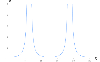
Figure 1. The typical phantom solution which begins at an initial Big-Rip singularity ($a\to\infty$, $\varrho,p\to\infty$) and terminates at final Big-Rip singularity ($a\to\infty$, $\varrho,p\to\infty$). Similarly as in the case of Big-Bang-to-Big-Crunch evolution many cycles are presumably admitted.

However, from the point of view of the observations (which support Hot Big-Bang models), the most interesting models are ”hybrid” models which begin with Big-Bang singularity and terminate at Big-Rip. Both types of matter (standard and phantom) are present during the whole evolution of the universe but an early evolution is dominated by the standard matter, while phantom dominates the late evolution of it. Of course, this means that there must have been a change during the evolution from deceleration to acceleration and this also might have happened quite recently (we will come to this point later). An explicit example of such an evolution for the dust ($w=0$) and phantom ($w=-4/3$) model is given in terms of Weierstrass elliptic functions as

$$\left(\frac{a}{a_{0}}\right)^{2} = \frac{4\Omega_{m0}{\cal P}(\eta)}{4\Omega_{ph0}{\cal P}^{2}(\eta)-\Omega_{m0}}~{},\hskip 28.45274ptd\eta=\sqrt{\frac{\Omega_{ph0}a_{0}}{a}}H_{0}dt~{},$$ (34)

where ${\cal P}(\eta)$ is the Weierstrass elliptic function, $\Omega_{m0},\Omega_{ph0}$ the density parameters of dust and phantom respectively.

3. Sudden future singularities of pressure and generalized sudden future singularities

Big-Rip may appear in some future time $t=t_{BR}$ analogously to Big-Crunch (which may appear in some future time $t=t_{BC}$), but because of growing acceleration it is sometimes called ”sudden”. However, we may have something more exotic in the future evolution of the universe - a singularity which presumably appears quite unexpectedly and does not violate all the energy conditions. The hint which allows for such a singularity is that we release the assumption about the imposition of the equation of state, i.e., we do not constrain pressure and the energy density in (4) and (5) by any equation like the one in (6). This enables quite independent time evolution of these physical quantities.

Suppose that we first choose the form of the scale factor as [21]

$$a(t) = A+\left(a_{s}-A\right)\left(\frac{t}{t_{s}}\right)^{m}-A\left(1-\frac{t}{t_{s}}\right)^{n}~{},$$ (35)

($A=$ const., $a_{s}\equiv a(t_{s})$) with its time derivatives

$$\dot{a} = \frac{m}{t_{s}}\left(a_{s}-A\right)\left(\frac{t}{t_{s}}\right)^{m-1}+A\frac{n}{t_{s}}\left(1-\frac{t}{t_{s}}\right)^{n-1}~{},$$ (36)

$$\ddot{a} = \frac{m\left(m-1\right)}{t_{s}^{2}}\left(a_{s}-A\right)\left(\frac{t}{t_{s}}\right)^{m-2}-A\frac{n(n-1)}{t_{s}^{2}}\left(1-\frac{t}{t_{s}}\right)^{n-2}~{}.$$ (37)

Choosing

$$1<n<2, 0<m\leq 1~{}.$$ (38)

we notice that the scale factor (35) vanishes and its derivatives (36)-(37) diverge at $t=0$ leading to a divergence of $\varrho$ and $p$ in (4)-(5) (Big-Bang singularity). On the other hand, the scale factor (35) and its first derivative (36) remain constant while its second derivative (37) diverge leading to a divergence of pressure in (5) only, with finite energy density (4), i.e.,

$$a = {\rm const.},\hskip 5.0pt\dot{a}={\rm const.},\hskip 5.0pt\ddot{a}\to-\infty,$$ (39)

$$\varrho = {\rm const.},\hskip 5.0ptp\to\infty,\hskip 5.0pt{\rm for}\hskip 5.0ptt\to t_{s}.$$ (40)

We then conclude that the future singularity appears and since it does not show up in the evolution of the scale factor, it is called ”sudden” future singularity (SFS) [21]. This singularity violates the dominant energy condition (16) [22], but does not violate any other energy condition.

Sudden future singularities may also be present in the inhomogeneous models of the universe where they may violate all the energy conditions. An explicit example of such a situation was given [23] for the inhomogeneous Stephani universe [24] with no spacetime symmetries with metric

$$ds^{2}~{} = ~{}-~{}\frac{a^{2}}{\dot{a}^{2}}\frac{a^{2}}{V^{2}}\left[\left(\frac{V}{a}\right)^{\cdot}\right]^{2}dt^{2}~{}+~{}\frac{a^{2}}{V^{2}}\left[dx^{2}~{}+dy^{2}~{}+~{}dz^{2}\right]~{},$$ (41)

where

$$V(t,x,y,z)=1+\frac{1}{4}k(t)\left\{\left[x-x_{0}(t)\right]^{2}+\left[y-y_{0}(t)\right]^{2}+\left[z-z_{0}(t)\right]^{2}\right\}~{},$$ (42)

and $a,x_{0},y_{0},z_{0}$ are arbitrary functions of time. It emerges that sudden future singularities are similar to finite-density singularities of pressure (FD) which appear in these Stephani models since they also do not admit a priori any equation of state. Besides, sudden future singularities are temporal pressure singularities which means that they may appear at an instant $t=t_{s}$ of the evolution, while finite-density singularities are spatial pressure singularities and they may exist somewhere in the universe nowadays. Sudden future singularities were also proven to exist in anisotropic models [26].

If we consider a general time derivative of an order $r$ for (35), i.e.,

$$a^{(r)} = \frac{m(m-1)(m-2)...(m-r+1)}{t_{s}^{r}}\left(a_{s}-A\right)\left(\frac{t}{t_{s}}\right)^{m-r}$$ (43)

$$+ (-1)^{r-1}A\frac{n(n-1)(n-2)...(n-r+1)}{t_{s}^{r}}\left(1-\frac{t}{t_{s}}\right)^{n-r}~{}$$

and replace the condition (38) by

$$N<n<N+1, 0<m\leq 1~{},$$ (44)

we realize that for any integer $N+1=r$ we have a singularity in the scale factor derivative $a^{(r)}$ (cf. (43)), and consequently in the appropriate pressure derivative $p^{(r-2)}$. This, for any $r\geq 3$, gives a sudden future singularity which fulfills all the energy conditions including the dominant one [25, 22]. These singularities are, for example, possible in the theories with higher-order curvature quantum corrections [27].

In fact, sudden future singularities are determined by a blow-up of the Riemann tensor and its derivatives rather than the scale factor (or its inverse) itself. This has an important consequence on the nature of these singularities in comparison with Big-Bang or Big-Rip singularities. Namely, the geodesics do not feel the sudden future singularities at all, since geodesic equations

$$\left(\frac{dt}{d\tau}\right)^{2} = A+\frac{P^{2}+KL^{2}}{a(t)}~{},$$ (45)

$$\frac{dr}{d\tau} = \frac{P_{1}cos{\phi}+P_{2}\sin{\phi}}{a(t)f(r)}~{},$$ (46)

$$\frac{d\phi}{d\tau} = \frac{L}{a(t)r^{2}}~{},$$ (47)

are not singular for $a_{s}=a(t_{s})=$ const. [28]. Here $(t,r,\theta=\pi/2,\phi)$ are coordinates of the Friedmann universe, $\tau$ is the proper time, $K=0,\pm 1$, $A,L,P^{2}=P_{1}^{2}+P_{2}^{2}$ are constants, and $f^{2}(r)=1/(1-Kr^{2})$. On the other hand, the geodesic deviation equation

$$\frac{D^{2}n^{\alpha}}{d\lambda^{2}}+R^{\alpha}_{~{}\beta\gamma\delta}u^{\beta}n^{\gamma}u^{\delta}=0~{},$$ (48)

where $n^{\alpha}$ is the deviation vector, and $u^{\beta}$ is the four-velocity vector ($\lambda$ - an affine parameter), feels this singularity since at $t=t_{s}$ we have the Riemann tensor $R^{\alpha}_{~{}\beta\gamma\delta}\to\infty$. This means point particles do not see sudden future singularities, but extended objects do in the sense that they may suffer infinite tidal forces although they may not be torn on crossing these singularities.

Besides, the spacetimes with sudden future singularities do not lead to geodesic incompletness - they are weak singularities according to the definitions of Tipler [29] and Królak [30]. In other words, sudden future singularities are not final state of the universe [28]. This situation is somewhat similar to what happens with finite density singularities in inhomogeneous Stephani models [31] although there instead of the extension of geodesics one has the extension of the hypersurfaces of constant time throughout these singularities.

In order to conclude, one has to stress that sudden future singularities and finite density singularities are totally different from Big-Rip singularities due to phantom since Big-Rip singularities are felt by geodesic equations and the evolution cannot be extended behind them. In other words, Big-Rip (like Big-Crunch) is really the final state of the evolution while sudden future singularity is not.

4. Statefinders and the diagnosis of the future state of the universe

From the discussion of the previous sections it is clear that all the types of singularities (Big-Bang, Big-Crunch, Big-Rip, sudden future singularities and generalized sudden future singularities) are related to a blow-up of the scale factor and its time derivatives

$$a(t),\dot{a}(t),\ddot{a}(t),\dddot{a}(t)\ldots~{},$$ (49)

and so to a blow-up of the energy density and pressure derivatives

$$\varrho(t),\dot{\varrho}(t),\ldots,p(t),\dot{p}(t),\ldots~{}.$$ (50)

Formally, we may translate all that into the observational characteristics of the expansion (statefinders) such as: the well-known Hubble parameter

$$H = \frac{\dot{a}}{a}~{},$$ (51)

and the deceleration parameter

$$q = -\frac{1}{H^{2}}\frac{\ddot{a}}{a}=-\frac{\ddot{a}a}{\dot{a}^{2}}~{},$$ (52)

together with the new characteristics: the jerk parameter [32]

$$j = \frac{1}{H^{3}}\frac{\dddot{a}}{a}=\frac{\dddot{a}a^{2}}{\dot{a}^{3}}~{},$$ (53)

and the ”kerk” (snap) parameter [33, 34]

$$k = -\frac{1}{H^{4}}\frac{\ddddot{a}}{a}=-\frac{\ddddot{a}a^{3}}{\dot{a}^{4}}~{},$$ (54)

the ”lerk” parameter

$$l = \frac{1}{H^{5}}\frac{a^{(5)}}{a}=\frac{a^{(5)}a^{4}}{\dot{a}^{5}}~{},$$ (55)

and ”merk”, ”nerk”, ”oerk”, ”perk” etc. parameters, of which a general term may be expressed as

$$x^{(i)} = (-1)^{i+1}\frac{1}{H^{i}}\frac{a^{(i)}}{a}=(-1)^{i+1}\frac{a^{(i)}a^{i-1}}{\dot{a}^{i+1}}~{},$$ (56)

and its time derivative reads as

$$\left(x^{(i)}\right)^{\cdot} = H\left[i(q+1)x^{(i)}-\left(x^{(i+1)}+x^{(i)}\right)\right]~{}.$$ (57)

Future predicted (”sudden”) blow-up of statefinders may easily be linked to an emergence of future singularities. In particular, this may be the proper signals for sudden future and generalized sudden future singularities.

The blow-up of statefinders can be read-off redshift-magnitude relation up to an appropriate order in redshift $z$ after using the redshift-magnitude relation applied to supernovae data [33, 34]

$$m-M=5\log_{10}{(cz)}-5\log_{10}{H_{0}}\left(\frac{5}{2}\log_{10}{e}\right)$$

$$\left\{(1-q_{0})z+\frac{1}{3}\left[\frac{q_{0}}{2}\left(\frac{9}{2}q_{0}+5\right)-j_{0}-\frac{7}{4}-\Omega_{K0}\right]z^{2}\right.$$ (58)

$$\left.\frac{1}{24}\left[2j_{0}\left(8q_{0}+5\right)-2k_{0}-q_{0}\left(7q_{0}^{2}+11q_{0}+23\right)+25\right.\right.$$

$$\left.\left.+4\Omega_{K0}\left(2q_{0}+1\right)\right]z^{3}+O(z^{4})\right\}~{}.$$

where $m$ is the observed magnitude, $M$ is the absolute magnitude, $c$ is the velocity of light, and $\Omega_{K0}=K/(H_{0}^{2}a_{0}^{2})$. From (4) it is clear that the jerk appears in the second order of the expansion and the ”kerk” appears in the third order of this expansion. In particular, the simple signal for Big-Bang, Big-Crunch or Big-Rip would be $\mid H_{0}\mid\to\infty$; for SFS would be $\mid q_{0}\mid\to\infty$, while for generalized SFS would be $\mid j_{0}\mid\to\infty$, $\mid k_{0}\mid\to\infty$ etc.

As it was mentioned in the Introduction, statefinders may be useful in determination of the current status of an equation of state (3) for the matter in the universe.

The most recent analysis of supernovae type Ia data [12] shows that

$$j_{0} > 0~{},$$ (59)

giving no hint about $k_{0}$. Apart from that it shows that acceleration of the universe started quite recently at redshift $z=0.46\pm 0.13$.

5. SFS avoidance - generalized energy conditions

From the analysis of the previous Section 4 we learned that Big-Crunch singularity in future may emerge despite all the energy conditions are fulfilled. On the other hand, Big-Rip may emerge despite the energy conditions are not fulfilled. Further, SFS emerges when only the dominant energy condition is violated, while generalized SFS do not lead to any violation of the energy conditions. This means that an applicability of the standard energy conditions of Hawking and Penrose [6] to cosmological models with more exotic properties is limited and so not very useful.

Because of that, one may consider some more general or different energy conditions which may be helpful in classification of singularities in contemporary cosmology based on the fundamental physical theories such as superstring theory, brane theory, or M-theory [36, 37, 38, 39, 40, 41].

First, let us consider the following higher-order dominant energy conditions [35]:

$$\dot{\varrho} \geq 0,\hskip 28.45274pt-\dot{p}\leq\dot{\varrho}\leq\dot{p}~{},$$ (60)

$$\ddot{\varrho} \geq 0,\hskip 28.45274pt-\ddot{p}\leq\ddot{\varrho}\leq\ddot{p}~{},$$ (61)

$$\dddot{\varrho} \geq 0,\hskip 28.45274pt-\dddot{p}\leq\dddot{\varrho}\leq\dddot{p}~{},$$ (62)

$$\ldots \ldots ..,\hskip 28.45274pt\ldots\ldots\ldots~{}.$$

The application of the formulas (4) and (5) together with the following equalities for the time derivatives of the Hubble parameter (51)

$$\dot{H} = -H^{2}\left(q+1\right)~{},$$ (63)

$$\ddot{H} = H^{3}\left(j+3q+2\right)~{},$$ (64)

$$\dddot{H} = -H^{4}\left[k+4j+3q\left(q+4\right)+6\right]~{},$$ (65)

$$\ddddot{H} = H^{5}\left[l+5k+10j(q+2)+30q(q+2)+24\right]~{},$$ (66)

allows us to write the higher-order energy conditions in terms of statefinders. The first-order dominant energy condition now reads as

$$\dot{\varrho}+\dot{p} = -2H^{3}\left({\rm{\bf j}}+3q+2+2\frac{K}{a^{2}H^{2}}\right)\geq 0~{}~{},$$ (67)

$$\dot{\varrho}-\dot{p} = -2H^{3}\left(-{\rm{\bf j}}+3q+4+4\frac{K}{a^{2}H^{2}}\right)\geq 0~{}~{},$$ (68)

the second-order reads as

$$\ddot{\varrho}+\ddot{p} = 2H^{4}\left[{\rm{\bf k}}+4j+3q(q+4)+6+2\frac{K}{a^{2}H^{2}}\left(q+3\right)\right]\geq 0~{}~{},$$ (69)

$$\ddot{\varrho}-\ddot{p} = 2H^{4}\left[-{\rm{\bf k}}+2j+3q(q+6)+12+4\frac{K}{a^{2}H^{2}}(q+3)\right]\geq 0~{}~{},$$ (70)

while the third-order reads as

$$\dddot{\varrho}+\dddot{p} =$$

$$- 2H^{5}\left[{\rm{\bf l}}+5k+10j(q+2)+30q(q+2)+24+2\frac{K}{a^{2}H^{2}}\left(j+9q+12\right)\right]\geq 0~{}~{},$$

$$\dddot{\varrho}-\dddot{p} =$$

$$- 2H^{5}\left[-{\rm{\bf l}}+k+2j(4q+11)+6(7q^{2}+17q+8)+4\left(j+9q+12\right)\frac{K}{a^{2}H^{2}}\right]\geq 0~{},$$

and so on. From these relations one can easily see that it is not possible to fulfill any generalized dominant energy condition if any of statefinders $j$, $k$, $l$, etc. is singular. This is due to the fact that the signs in the appropriate expressions in front of statefinders are the opposite. This gives a conclusion that the violation of the higher-order dominant energy conditions can be good signals for the emergence of the generalized sudden future singularities.

In a similar manner one is able to consider the higher-order null, weak and strong energy conditions as follows

$$\dot{\varrho}+\dot{p} = -2H^{3}\left({\rm{\bf j}}+3q+2+2\frac{K}{a^{2}H^{2}}\right)\geq 0~{},$$ (73)

$$\dot{\varrho}+\dot{p} = -2H^{3}\left({\rm{\bf j}}+3q+2+2\frac{K}{a^{2}H^{2}}\right)\geq 0~{},\hskip 14.22636pt\dot{\varrho}\geq 0~{},$$ (74)

$$\dot{\varrho}+3\dot{p} = -6H^{3}({\rm{\bf j}}+q)\geq 0~{},\hskip 14.22636pt\dot{\varrho}+\dot{p}=-2H^{3}\left({\rm{\bf j}}+3q+2+2\frac{K}{a^{2}H^{2}}\right)\geq 0~{},$$ (75)

$$\ldots+\ldots = \ldots\ldots\geq 0~{},$$

and so on.

After having a closer look at them it emerges that these higher-order energy conditions are not always very useful in order to determine the future fate of the Universe.

However, some hybrid energy conditions may work for that. For example an energy condition [26]

$$\alpha\varrho > \dot{p}~{},$$ (76)

with $\alpha=$ const., which in terms of statefinders gives

$$j > \left(1-\frac{3\alpha}{2H}\right)\left(1+\frac{K}{a^{2}H^{2}}\right)~{},$$ (77)

may prevent the emergence of sudden future singularity singularity for $N=2$ in (44).

6. Conclusions

In view of the discussion performed in this paper one has the following remarks.

Firstly, the future state of the universe may be more sudden and violent. It means that the universe may terminate either in a sudden future singularity or in a Big-Rip singularity and this is totally different from our earlier expectations that it could terminate in an asymptotically de Sitter state or in a Big-Crunch.

Secondly, these new future singularities (Big-Rip and SFS) should not be confused - they have totally different properties with respect to geodesic completness. In particular, one can extend the evolution of the universe through a sudden future singularity, while it is not possible to do so for a Big-Rip.

Thirdly, statefinders (Hubble, deceleration, jerk, kerk etc.) may be useful to diagnose the future state of the universe. By this we mean the emergence of sudden future singularities, the emergence of generalized sudden future singularities, the evolution of the cosmic equation of state $w=w(t)$ etc.

Finally, the new energy conditions may be introduced for the sake of the proper signal for generalized sudden future singularities, or (on the contrary), for the sake of the avoidance of sudden future singularities, or generalized sudden future singularities.

This work was partially supported by the Polish Ministry of Education and Science grant No 1 P03B 043 29 (years 2005-2007).

References

- [1] E. Hubble, Proc. Nat. Acad. Sci. USA 15, 168 (1929).
- [2] G. Gamow, Phys. Rev. 70, 572 (1946).
- [3] A.A. Penzias and R.W. Wilson, Astroph. J. 142, 419 (1965).
- [4] J. Polchinski, Rev. Mod. Phys. 68, 1245 (1996).
- [5] J. Polchinski, String Theory (Cambridge University Press, Cambridge, 1998).
- [6] Hawking, S.W., Ellis, G.F.R., The Large-scale Structure of Space-time, (Cambridge University Press, Cambridge, 1999) .
- [7] S. Perlmutter et al., Astroph. J. 517, 565 (1999); A. G. Riess et al. Astron. J. 116, 1009 (1998); A.G. Riess et al., Astroph. J. 560, 49 (2001); astro-ph/0207097.
- [8] A. Einstein, Preuss. Akad. Wiss. Berlin, Sitzber, 142 (1917).
- [9] A. Vilenkin, Phys. Rep. 121, 265 (1985); T. Vachaspati, and A. Vilenkin, Phys. Rev. D 35, 1131 (1987).
- [10] M.P. Da̧browski, and J. Stelmach, Astron. Journ. 97, 978 (1989) (astro-ph/0410334).
- [11] J.L. Tonry et al., Astroph. J. 594, 1 (2003); M. Tegmark et al., Phys. Rev. D 69, 103501 (2004).
- [12] A.G. Riess et al. Astrophys. J. 607, 665 (2004).
- [13] R.R. Caldwell, Phys. Lett. B 545, 23 (2002); S. Hannestad and E. Mörstell, Phys. Rev. D 66, 063508 (2002); P.H. Frampton, Phys. Lett. B 562, 139 (2003); S. Nojiri and D. Odintsov, Phys. Lett. B 562, 147 (2003).
- [14] M.P. Da̧browski, T. Stachowiak and M. Szydłowski, Phys. Rev. D 68, 103519 (2003).
- [15] S.M. Carroll, M. Hofman, and M. Trodden, Phys. Rev. D 68, 023509 (2003); S.D.H. Hsu, A. Jenkins, and M.B. Wise, Phys. Lett. B 597, 270 (2004); J.M. Cline, S. Jeon, and G.D. Moore, hep-ph/0311312; I.Ya. Aref’eva, A.S. Koshelev, and S.Yu. Yernov, astro-ph/0507067.
- [16] C. Csaki, N. Kaloper, and J. Terning, Ann. Phys. (N.Y.) 317, 410 (2005).
- [17] V.A. Belinsky, E.M. Lifshitz, and I.M. Khalatnikov, Sov. Phys. Usp. 102, 745 (1971); J.D. Barrow, Phys. Rep. 85, 1 (1982).
- [18] K.A. Meissner and G. Veneziano, Phys. Lett. B 267, 33 (1991); Mod. Phys. Lett. A 6, 1721 (1991).
- [19] L.P. Chimento and R. Lazkoz, Phys. Rev. Lett. 91, 211301 (2003).
- [20] J.E. Lidsey, Phys. Rev. D 70, 041302 (2004).
- [21] J.D. Barrow, Class. Quantum Grav. 21, L79 (2004).
- [22] K. Lake, Class. Quantum Grav. 21, L129 (2004).
- [23] M.P. Da̧browski, Phys. Rev. D 71, 103505 (2005).
- [24] H. Stephani, Commun. Math. Phys. 4, 137 (1967).
- [25] J.D. Barrow, Class. Quantum Grav. 21, 5619 (2004).
- [26] J.D. Barrow and Ch. Tsagas, Class. Quantum Grav. 22, 1563 (2005).
- [27] S. Nojiri and S.D. Odintsov, Phys. Lett. B 595, 1 (2004); S. Nojiri, S.D. Odintsov and S. Tsujikawa, Phys. Rev. D 71,063004 (2005).
- [28] L. Fernandez-Jambrina and R. Lazkoz, Phys. Rev. D 70, 121503 (2004).
- [29] F.J. Tipler, Phys. Lett. A 64, 8 (1977).
- [30] A. Królak, Class. Quantum Grav. 3, 267 (1986).
- [31] M.P. Da̧browski, Journ. Math. Phys. 34, 1447 (1993).
- [32] E.R. Harrison, Nature 260, 591 (1976); P.T. Landsberg, Nature 263, 217 (1976); T. Chiba, Prog. Theor. Phys. 100, 1077 (1998); Yu. Shtanov and V. Sahni, Class. Quantum Grav. 19, L101 (2002); U. Alam, V. Sahni, T.D. Saini, and A.A. Starobinsky, Mon. Not. R. Astron. Soc. 344, 1057 (2003); V. Sahni, T.D. Saini, A.A. Starobinsky, and U. Alam, JETP Lett. 77, 201 (2003); M. Visser, Class. Quantum Grav. 21, 2603 (2004).
- [33] R.R. Caldwell and M. Kamionkowski, JCAP 0409, 009 (2004).
- [34] M.P. Da̧browski and T. Stachowiak, Ann. Phys. N.Y. to appear (hep-th/0411199).
- [35] M.P. Da̧browski, Phys. Lett. B 625, 184 (2005).
- [36] P. Hořava and E. Witten, Nucl. Phys. B460, 506 (1996); ibid B475, 94 (1996).
- [37] L. Randall and R. Sundrum, Phys. Rev. Lett., 83, 3370 (1999); ibid 83, 4690.
- [38] J.E. Lidsey, D.W. Wands, and E.J. Copeland, Phys. Rept. 337, 343 (2000).
- [39] M. Gasperini and G. Veneziano, Phys. Rep. 373, 1 (2003).
- [40] F. Quevedo, Class. Quantum Grav. 19, 5721 (2002).
- [41] J. Khoury, P.J. Steinhardt and N. Turok, Phys. Rev. Lett. 92, 031302 (2004).
- [42] H. Štefančić, Phys. Lett. B586 , 5 (2004); ibidem B595, 9 (2004); Phys. Rev. D71 , 084024 (2004).
- [43] H.K. Jassal, J.S. Bagla, T. Padmanabhan, Mon. Not. Roy. Astron. Soc. 356, L11 (2005); R.R. Caldwell and M. Doran, astro-ph/0501104.
- [44] V.K. Onemli, R.P. Woodard, Class. Quantum. Grav. 19, 4607 (2002); Phys. Rev. D70, 107301 (2004).