One-dimensional Hybrid Approach to Extensive Air Shower Simulation

Abstract

An efficient scheme for one-dimensional extensive air shower simulation and its implementation in the program conex are presented. Explicit Monte Carlo simulation of the high-energy part of hadronic and electromagnetic cascades in the atmosphere is combined with a numeric solution of cascade equations for smaller energy sub-showers to obtain accurate shower predictions. The developed scheme allows us to calculate not only observables related to the number of particles (shower size) but also ionization energy deposit profiles which are needed for the interpretation of data of experiments employing the fluorescence light technique. We discuss in detail the basic algorithms developed and illustrate the power of the method. It is shown that Monte Carlo, numerical, and hybrid air shower calculations give consistent results which agree very well with those obtained within the corsika program.

1 Introduction

Monte Carlo (MC) simulation of extensive air showers (EAS) is the most common method to calculate detailed theoretical predictions needed for interpreting experimental data of air shower arrays or fluorescence light detectors. However, for primary particles of very high energy, straight-forward MC simulation is not a viable option because of the unreasonably large computing time required. The situation can be improved by applying some weighted sampling algorithms, like the so-called “thinning” method [1], i.e. treating explicitly only a small portion of all shower particles and assigning each particle a corresponding weight factor. Although this approach allows the reduction of EAS calculation times to practically affordable values, it comes soon to its limits. The summation of particle contributions with very large weights creates significant artificial fluctuations for EAS observables of interest [2, 3, 4]. Imposing maximum weight limitations to ensure high simulation quality [4], on the other hand, prevents one from using less detailed sampling and correspondingly from further speeding-up the calculation process. A possible alternative procedure is to describe EAS development numerically, based on the solution of the corresponding cascade equations [5, 6, 7]. Combining this with an explicit MC simulation of the most high-energy part of an air shower allows one to obtain accurate results both for average EAS characteristics and for their fluctuations [8].

In this article we describe a new EAS simulation program of such a hybrid type, called conex. In conex the MC treatment of above-threshold particle cascading is realized in the standard way and does not differ significantly from the implementation in e.g. corsika [9]. On the other hand, the numerical description of lower energy sub-cascades is based on the solution of hadronic cascade equations, using an updated algorithm of Ref. [7], and a newly developed procedure for the solution of electro-magnetic (e/m) cascade equations. The corresponding algorithms are characterized by high efficiency and good accuracy even if a comparatively crude binning with respect to particle energy and depth position is used. Furthermore, by accounting for neutrino production in addition to the typically considered particles, conex can also be used for the calculation of ionization energy deposit profiles.

The numeric solution of cascade equations can be replaced, in principle, by a pre-tabulation of the characteristics of secondary sub-cascades, obtained via an iterative MC procedure [10, 11, 12]. An example of a combined approach, extended to a three-dimensional EAS simulation, is described in Ref. [13], where hadronic sub-cascades are treated using the method of Ref. [7] and e/m sub-cascades are tabulated using the egs4 MC program [14].

The approach presented in the current work does not require any pre-tabulation of particle cascades and is characterized by high efficiency and large flexibility. It can be applied to various initial conditions, i.e. a wide range of energies and angles of incidence of a primary particle, including the case of upward-going showers, as well as arbitrary parameterizations of the atmosphere of the Earth. These features make conex ideally suited for applications related to the event-by-event based analysis of EAS data, in particular, of fluorescence light based measurements.

This is the first paper in a series in which we will investigate various features of EAS and their relation to the characteristics of hadronic multiparticle production. In this work, we shall present the hybrid simulation scheme in detail, leaving the study of shower predictions to a forthcoming article.

The outline of the paper is as follows. Section 2 describes the calculation scheme and its basic procedures. In Section 3 we show some examples of calculated EAS characteristics and investigate the accuracy and efficiency of the method comparing the hybrid approach with pure MC or numerical procedures. The reliability of the predictions is checked by a detailed comparison with corsika results. Finally, a summary is given in Section 4 and both potential applications of the program and the prospects for its further development are discussed.

2 Calculation scheme

2.1 Physics overview

The calculation scheme consists of two main stages: an explicit MC simulation of the cascade for particles with energies above some chosen threshold $E_{\rm thr}$ (being a free parameter of the scheme) and a solution of nuclear-electro-magnetic cascade equations for sub-cascades of smaller energies. Both MC and numerical parts are characterized by the same physics content, as described below.

In the hadronic cascade one follows the propagation, interaction and decay (where applicable) of (anti-) nucleons, charged pions, charged and neutral kaons; all other types of hadrons produced in interactions and decays are assumed to decay immediately. Particle interactions in the MC part are treated within a chosen high energy hadronic interaction model (implemented are nexus 3.97 [15, 16, 17], qgsjet 01 [18, 19] and ii [20, 21, 22], and sibyll 2.1 [23, 24, 25]), decays are simulated using the corresponding routines of the nexus model. The same models are used to pre-calculate secondary particle spectra for later use in the numerical treatment of hadronic cascade equations. Optionally, below some energy $E_{\rm low}^{\rm had}\sim 100$ GeV, gheisha [26] is employed as low-energy hadronic interaction model.

The MC treatment of the e/m cascade is realized by means of the egs4 code [14], supplemented by an account of the Landau-Pomeranchuk-Migdal (LPM) effect [27, 28, 29] for ultra-high energy electrons (positrons) and photons. The simulation of photonuclear interactions and muon pair production was added to the egs package closely following the corsika implementation [9]. The system of coupled e/m cascade equations is based on the same interaction processes as implemented in the MC, using Bethe-Heitler cross sections for the bremsstrahlung and pair production with energy-dependent correction factors according to Storm and Israel [30], the Klein-Nishina formula for the Compton process, and accounting for Moeller and Bhabha processes as well as for positron-electron annihilation (see, for example [14, 31]). Both LPM suppression and photo-effect are neglected in the e/m cascade Eqs., as the latter are employed in the energy ranges where these processes are not important. Ionization losses of electrons and positrons are described by the Bethe-Bloch formula with corrections to account for the density effect [32].

High energy interactions of muons (bremsstrahlung, pair production and muon-nuclear interaction [33, 34, 35, 36, 37]) are taken into account in the MC part but are neglected in the cascade Eqs.

In general, an individual shower is simulated as follows. One starts with the primary particle of given energy, direction and initial position in the atmosphere (by default, at 100 km above sea level, if no special geometry is required, e.g. up-going showers). The initial particle direction thus defines the position of the “true” shower axis, in the following referred to as the “shower trajectory”. For a hadron as primary particle, one simulates the hadronic cascade explicitly, recording all secondary particles at a number of pre-chosen depth levels and energy intervals, until all produced secondaries have an energy lower than the threshold $E_{\rm thr}$. The levels are defined with respect to the projected depth $X$, i.e. the slant depth for the particle position projected to the initial shower axis (shower trajectory), as described in more detail in the Appendix. All sub-threshold hadrons/muons and e/m particles are filled into energy-depth tables that form the “source terms” for the cascade equations. In parallel, the above-threshold e/m particles are transferred to egs4 for simulating the e/m particle cascade in a similar way, with all sub-threshold e/m particles being added to the e/m source terms.

In the next step the hadronic cascade at energies below $E_{\rm thr}$ is calculated numerically for the first depth level using the corresponding cascade equations and initial conditions specified by the source terms. As the result, one obtains discretized energy spectra of hadrons of different types at the next depth level. All sub-threshold e/m particles produced at this stage are added to the e/m source term. Then sub-threshold e/m cascades are calculated by solving the corresponding e/m cascade equations for the given initial conditions. Hadrons due to photonuclear interaction and pair-produced muons that are generated in the numerical solution of the e/m cascade Eqs. are added to the hadronic source term of the next slant depth level. This procedure is repeated for the following depth levels, each time using the hadronic and e/m source terms of the previous level.

Ultra-high energy e/m particles can undergo geomagnetic pair production and bremsstrahlung well above the atmosphere of the Earth [38, 39, 40]. Therefore, in case of the primary particle being a photon or an electron, the simulation process starts with the calculation of possible interactions with the geomagnetic field using the preshower code [41] and the above described procedure is applied to the secondary particles.

2.2 Hadronic cascade equations

The backbone of a hadron-initiated extensive air shower is the hadronic cascade which develops via particle propagation, decay, and interaction with air nuclei of both the initial particle and of produced secondary hadrons. The corresponding integro-differential equations are given by [7] (see also [13])

$$\frac{\partial\left.h_{a}(E,X)\right|_{T}}{{\partial X}} = -\frac{\left.h_{a}(E,X)\right|_{T}}{\lambda_{a}(E)}-\left.h_{a}(E,X)\right|_{T}\frac{\left|\frac{dL}{dX}\right|_{T}}{\tau_{a}(E)\,c}+\frac{\partial}{\partial E}\left(\beta_{a}^{{\rm ion}}(E)\left.h_{a}(E,X)\right|_{T}\right)$$ (1)

$$+\sum_{d}\int_{E}^{E_{\max}}\!dE^{\prime}\;\left.h_{d}(E^{\prime},X)\right|_{T}\;\left[\frac{W_{d\rightarrow a}(E^{\prime},E)}{\lambda_{d}(E^{\prime})}+D_{d\rightarrow a}(E^{\prime},E)\frac{\left|\frac{dL}{dX}\right|_{T}}{\tau_{d}(E^{\prime})\,c}\right]$$

$$+\left.S_{a}^{{\rm had}}(E,X)\right|_{T},$$

where $\left.h_{a}(E,X)\right|_{T}$ are the differential energy spectra of hadrons of type $a$ with energy $E$ at depth position $X$ along a given straight line trajectory $T$ (in the following the $T$-symbol will be omitted), $\beta_{a}^{{\rm ion}}(E)=-dE_{a}/dX$ is the ionization energy loss of particle $a$ per depth unit. A muon is treated like a hadron, but without interaction term.

The first term in the r.h.s. of Eq. (1) represents the decrease of hadron number due to interactions with air nuclei

$$\frac{dh_{a}}{dX}=-\frac{h_{a}}{\lambda_{a}},$$ (2)

with the corresponding mean free path $\lambda_{a}=m_{\mathrm{air}}/\sigma_{\mathrm{inel}}^{a-{\rm air}}$, where $m_{{\rm air}}$ is the average mass of air molecules and $\sigma_{\mathrm{inel}}^{a-{\rm air}}$ is the hadron $a$ - air nucleus inelastic cross section.

The second term describes particle decay, with the decay rate on a path $dL$ being

$$dh_{a}=-h_{a}\>\frac{dL}{\tau_{a}\,c},$$ (3)

where $\tau_{a}$ is the life time of hadron $a$ in the lab. system, related to the proper life time $\tau_{a}^{(0)}$ by $\tau_{a}=\tau_{a}^{(0)}\,E/m_{a}$, with $m_{a}$ being the hadron mass and $c$ the velocity of light. From the definition of slant depth (28) follows

$$\left|\frac{dL}{dX}\right|=\frac{1}{\rho_{{\rm air}}(X)}.$$ (4)

The third term in Eq. (1) takes into account particle ionization energy losses and the integral term in Eq. (1) represents the production of particles of type $a$ in interactions and decays of higher energy parents of type $d$, with $W_{d\rightarrow a}(E^{\prime},E)$, $D_{d\rightarrow a}(E^{\prime},E)$ being the corresponding inclusive spectra of secondaries.

Finally, the so-called source term $S_{a}^{{\rm had}}(E,X)$ defines the initial conditions and is determined during the MC simulation of above-threshold particle cascading. It consists of contributions of all sub-threshold hadrons produced at that stage

$$S_{a}^{{\rm had}}(E,X)=S_{a}^{{\rm MC\rightarrow had}}(E,X)=\sum_{i=1}^{N_{{\rm source}}^{{\rm had}}}\delta_{d_{i}}^{a}\,\delta(E-E_{i})\,\delta(X-X_{i}),$$ (5)

with $d_{i}$, $E_{i}$, $X_{i}$ being type, energy, and depth position of the source particles.

The numerical method of solving the hadronic cascade equations is similar to the approach of [7] and is summarized in Appendix 5.2.

2.3 Electro-magnetic cascade equations

The e/m cascade development can be described by the following system of integro-differential equations (see, for example, [31])

$$\frac{\partial l_{e^{-}}\!(E,X)}{{\partial X}} = -\sigma_{e^{-}}\!(E)\>l_{e^{-}}\!(E,X)+\frac{\partial}{\partial E}\left(\beta_{e^{-}}^{{\rm ion}}(E)l_{e^{-}}(E,X)\right)$$ (6)

$$+\int_{E}^{E_{\max}}\!dE^{\prime}\,\left[l_{e^{-}}\!(E^{\prime},X)\,W_{e^{-}\rightarrow e^{-}}\!(E^{\prime},E)+l_{e^{+}}\!(E^{\prime},X)\right.$$

$$\times\left.\,W_{e^{+}\rightarrow e^{-}}\!(E^{\prime},E)+l_{\gamma}\!(E^{\prime},X)\,W_{\gamma\rightarrow e^{-}}\!(E^{\prime},E)\right]+S_{e^{-}}^{{\rm e/m}}\!(E,X)$$

$$\frac{\partial l_{e^{+}}\!(E,X)}{{\partial X}} = -\sigma_{e^{+}}\!(E)\>l_{e^{+}}\!(E,X)+\frac{\partial}{\partial E}\left(\beta_{e^{+}}^{{\rm ion}}(E)l_{e^{+}}(E,X)\right)$$ (7)

$$+\int_{E}^{E_{\max}}\!dE^{\prime}\,\left[l_{e^{+}}\!(E^{\prime},X)\,W_{e^{+}\rightarrow e^{+}}\!(E^{\prime},E)\right.$$

$$+\left.l_{\gamma}\!(E^{\prime},X)\,W_{\gamma\rightarrow e^{+}}\!(E^{\prime},E)\right]+S_{e^{+}}^{{\rm e/m}}\!(E,X)$$

$$\frac{\partial l_{\gamma}\!(E,X)}{{\partial X}} = -\sigma_{\gamma}\!(E)\>l_{\gamma}\!(E,X)+\int_{E}^{E_{\max}}\!dE^{\prime}$$ (8)

$$\times\left[l_{\gamma}\!(E^{\prime},X)W_{\gamma\rightarrow\gamma}\!(E^{\prime},E)+l_{e^{-}}\!(E^{\prime},X)\,W_{e^{-}\rightarrow\gamma}\!(E^{\prime},E)\right.$$

$$+\left.l_{e^{+}}\!(E^{\prime},X)\,W_{e^{+}\rightarrow\gamma}\!(E^{\prime},E)\right]+S_{\gamma}^{{\rm e/m}}\!(E,X),$$

where $l_{a}\!(E,X)$ ($a=e^{-},\,e^{+},\,\gamma$) are energy spectra of electrons, positrons, and photons at depth $X$, $\sigma_{a}\!(E)$ are interaction cross sections (in units area/mass, see Sec. 2.2)

$$\sigma_{e^{-}} = \sigma_{\rm(bremsstrahlung)}+\sigma_{\rm(Moeller)}$$

$$\sigma_{e^{+}} = \sigma_{\rm(bremsstrahlung)}+\sigma_{\rm(Bhabha)}+\sigma_{\rm(annihilation)}$$

$$\sigma_{\gamma} = \sigma_{\rm(pair\leavevmode\nobreak\ production)}+\sigma_{\rm(Compton)}+\sigma_{\rm(photonuclear)}+\sigma_{\rm(muon\leavevmode\nobreak\ pair)},$$ (9)

and $W_{d\rightarrow a}(E^{\prime},E)$ are corresponding differential energy spectra of secondary particles

$$W_{e^{-}\rightarrow e^{-}}\!(E^{\prime},E)=W_{e^{-}\rightarrow e^{-}}^{{\rm brems}}\!(E^{\prime},E)+W_{e^{-}\rightarrow e^{-}}^{{\rm Moeller}}\!(E^{\prime},E)$$

$$W_{e^{+}\rightarrow e^{+}}\!(E^{\prime},E)=W_{e^{-}\rightarrow e^{-}}^{{\rm brems}}\!(E^{\prime},E)+W_{e^{+}\rightarrow e^{+}}^{{\rm Bhabha}}\!(E^{\prime},E)$$

$$W_{\gamma\rightarrow\gamma}\!(E^{\prime},E)=W_{\gamma\rightarrow\gamma}^{{\rm Compton}}\!(E^{\prime},E)$$

$$W_{e^{-}\rightarrow\gamma}\!(E^{\prime},E)=W_{e^{-}\rightarrow e^{-}}^{{\rm brems}}\!(E^{\prime},E^{\prime}-E)$$

$$W_{e^{+}\rightarrow\gamma}\!(E^{\prime},E)=W_{e^{-}\rightarrow e^{-}}^{{\rm brems}}\!(E^{\prime},E^{\prime}-E)+W_{e^{+}\rightarrow\gamma}^{{\rm annih}}\!(E^{\prime},E)$$

$$W_{e^{+}\rightarrow e^{-}}\!(E^{\prime},E)=W_{e^{+}\rightarrow e^{+}}^{{\rm Bhabha}}\!(E^{\prime},E^{\prime}-E)$$

$$W_{\gamma\rightarrow e^{-}}\!(E^{\prime},E)=W_{\gamma\rightarrow e^{-}}^{{\rm pair}}\!(E^{\prime},E)+W_{\gamma\rightarrow\gamma}^{{\rm Compton}}\!(E^{\prime},E^{\prime}-E)$$

$$W_{\gamma\rightarrow e^{+}}\!(E^{\prime},E)=W_{\gamma\rightarrow e^{-}}^{{\rm pair}}\!(E^{\prime},E).$$ (10)

Here $\sigma_{\rm(Moeller)}$ and $\sigma_{\rm(Bhabha)}$ correspond to the process of $\delta$-electron knock out above some energy threshold $E_{\min}^{{\rm e/m}}$

$$\sigma_{e^{-/+}}^{{\rm Moeller/Bhabha}}\!(E)=\int_{E_{\min}^{{\rm e/m}}}^{E}\!dE^{\prime}\,W_{e^{-/+}\rightarrow e^{-/+}}^{{\rm Moeller/Bhabha}}\!(E,E^{\prime}),$$ (11)

whereas the contribution of those processes below $E_{\min}^{{\rm e/m}}$ is treated as continuous energy losses and constitutes a part of $\beta_{{\rm ion}}^{e^{\pm}}\!(E)$

$$\beta_{e^{\pm}}^{{\rm ion}}\!(E)=\left.-\frac{dE_{e^{\pm}}}{dX}\right|_{{\rm ionization}+\delta(<E_{\min}^{{\rm e/m}})}.$$ (12)

The bremsstrahlung cross section diverges due to the characteristic infra-red singular behavior $1/E^{\prime}$ of the secondary photon spectrum $W_{e^{-}\rightarrow\gamma}^{{\rm brems}}\!(E,E^{\prime})=W_{e^{-}\rightarrow e^{-}}^{{\rm brems}}\!(E,E-E^{\prime})$ and normaly requires to introduce some low energy cutoff. The sub-cutoff photon emission could be treated as continuous “radiation” energy losses as is done in egs4 [14]. However, this is not necessary in our calculation scheme as is shown in Appendix 5.3, where the numerical solution is presented.

2.4 Photonuclear effect and muon pair production

To take into account hadron and muon production by photons, two additional terms are introduced that couple e/m and hadronic cascade equations via source terms. Photoproduction of hadrons, i.e.  photonuclear interaction, is implemented using the cross section of Ref. [42]. Particle production distributions are approximated by those of $\pi^{0}$-air interactions. Then the corresponding source term can be written as

$$S_{a}^{{\rm em\rightarrow had}}(E,X)=\int_{E}^{E_{\max}}\!dE^{\prime}\;l_{\gamma}(E^{\prime},X)\;W_{\pi^{0}\rightarrow a}(E^{\prime},E)\,\sigma_{\gamma}^{\mathrm{photonuc}}(E^{\prime}),$$ (13)

where $W_{\pi^{0}\rightarrow a}(E^{\prime},E)$ is defined in analogy to Eq. (10). With a small cross section, a photon can also produce a $\mu^{+}\mu^{-}$ pair. This gives another contribution to the hadronic source term

$$S_{\mu}^{{\rm em\rightarrow\mu}}(E,X)=\int_{E}^{E_{\max}}\!dE^{\prime}\;l_{\gamma}(E^{\prime},X)\;W_{\gamma\rightarrow\mu}(E^{\prime},E)\,\sigma_{\gamma}^{\mathrm{mu-pair}}(E^{\prime}).$$ (14)

Finally the source term defined in Eq. (5) becomes

$$S_{a}^{{\rm had}}(E,X)=S_{a}^{{\rm MC\rightarrow had}}(E,X)+S_{a}^{{\rm em\rightarrow had}}(E,X)+S_{\mu}^{{\rm em\rightarrow\mu}}(E,X)\;\delta_{a}^{\mu}\,.$$ (15)

3 Applications

In the following we demonstrate the reliability of the conex code by comparing predictions for shower observables calculated with cascade Eqs. and the full hybrid scheme to that of MC simulations. As conex can also run in pure MC mode, both conex and corsika are used for calculating the MC predictions.

If not specified otherwise, the calculations were performed using the qgsjet model for hadronic interactions at energies $E>E_{{\rm low}}^{{\rm had}}=80$ GeV and gheisha model for $E<E_{{\rm low}}^{{\rm had}}$. Our default choice for the cutoff between the MC and the numerical parts is $E_{{\rm thr}}=10^{-2}E_{0}$, $E_{0}$ being the energy of the primary particle. The default energy grid for solving the cascade Eqs. is 30 bins per energy decade ($d_{E}=30$) for hadrons and e/m particles and the slant depth binning has a 5 g/cm² elementary step ($\Delta X$). When applying the hybrid scheme, high energy particles are treated in MC. As a consequence the energy transfer from hadronic to e/m particles is more precise, allowing us to use larger bins, i.e. 20 bins per energy decade and a 10 g/cm² slant depth step size.

3.1 Hadronic shower component

In Fig. 1 we investigate the stability of our scheme and compare both longitudinal profiles of nucleons and charged pions and their energy spectra at 500 g/cm² for different choices of energy and depth discretization. Results only change significantly for very large discretization intervals.

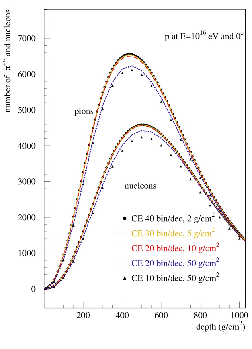
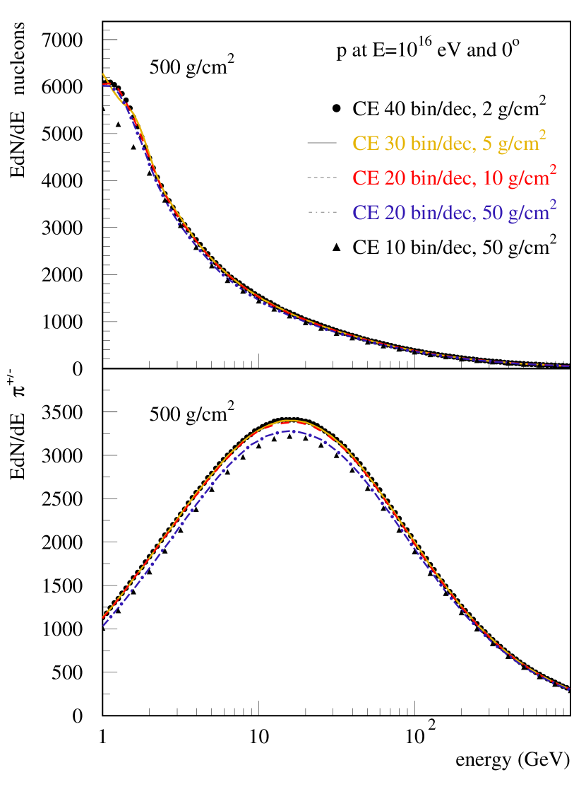
Figure 1: Average hadronic shower size profiles (left panel) and energy spectra at $X=500$ g/cm² (right panel) of nucleons and charged pions for proton-initiated vertical ($\theta=0^{{\rm o}}$) showers of $10^{16}$ eV. Compared are the results of solving numerically the system of cascade equations (CE) with different discretization bin sizes in energy and depth.

In Fig. 2 we plot similar characteristics of charged pions and muons for $10^{18}$ eV proton-initiated showers simulated with qgsjet 01 at high energy and gheisha at low energy. The results are compared to corsika predictions. The agreement between the results from the different conex calculation methods as well as corsika simulations is very good.

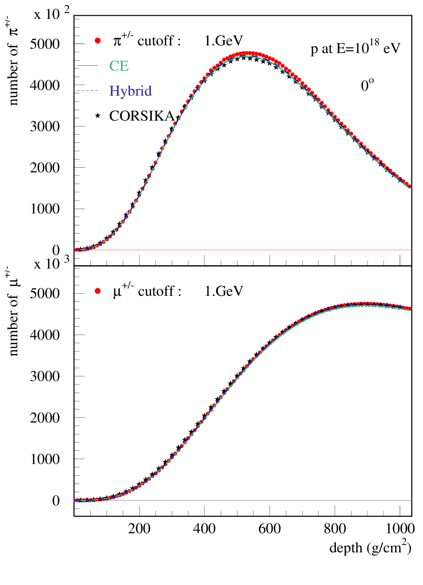
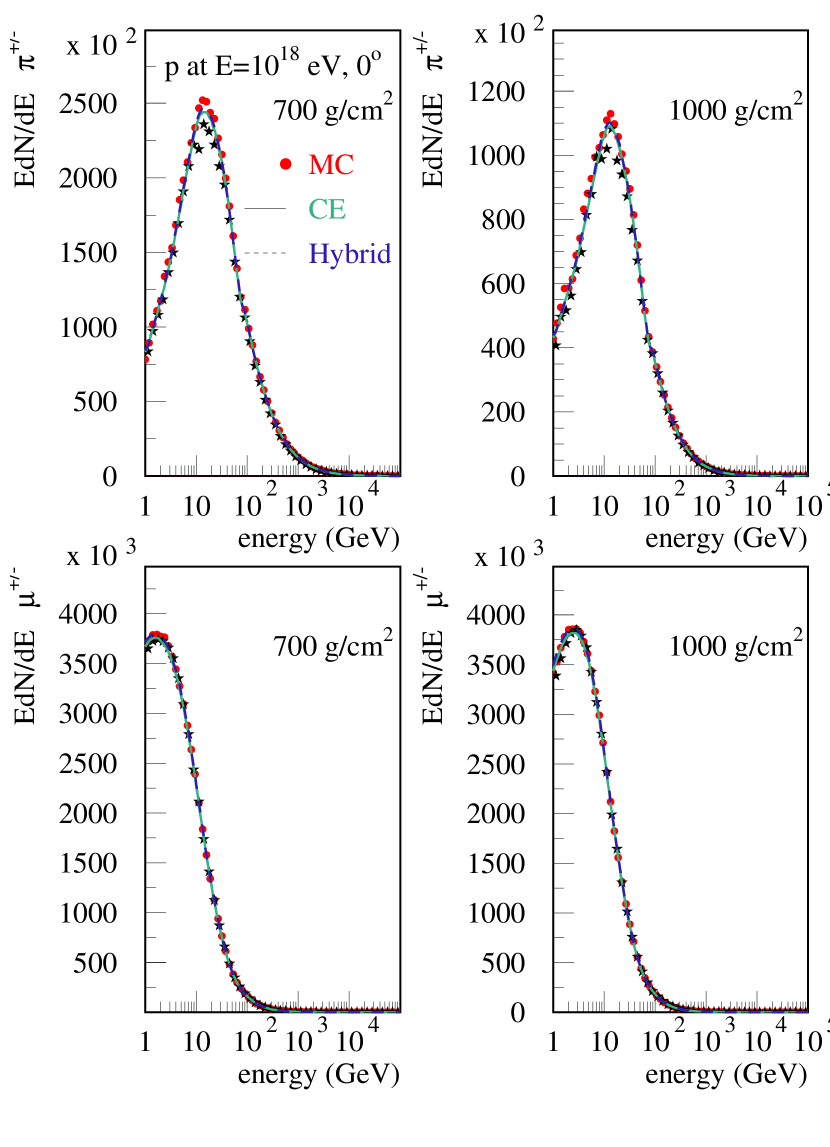
Figure 2: Average longitudinal shower size profiles (left panel) and energy spectra (right panel) of charged pions and muons with energies above 1 GeV. The calculations were done for proton-initiated vertical showers of $10^{18}$ eV. Compared are the predictions obtained with conex applying the hybrid (dashed line), pure MC (points) and numerical calculation (full line) schemes. In addition CORSIKA predictions are shown as symbols (stars).

3.2 Electromagnetic shower component

The longitudinal profiles of electrons, positrons, and photons for a $10^{14}$ eV vertical photon-initiated shower are shown in Fig. 3 (left panel). The shower size profiles are given for the cutoff energies $E_{\min}^{{\rm e/m}}=$1 MeV, 1000 MeV using again the hybrid, pure MC, and cascade equation approaches.

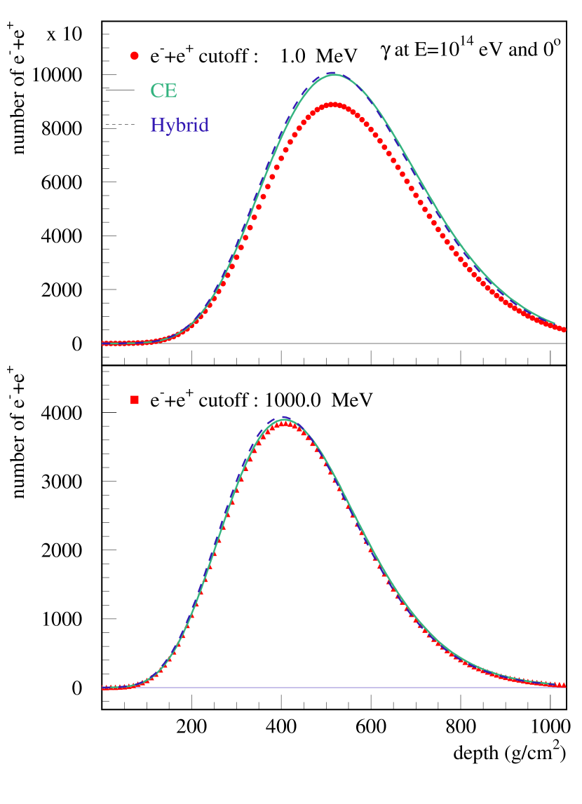
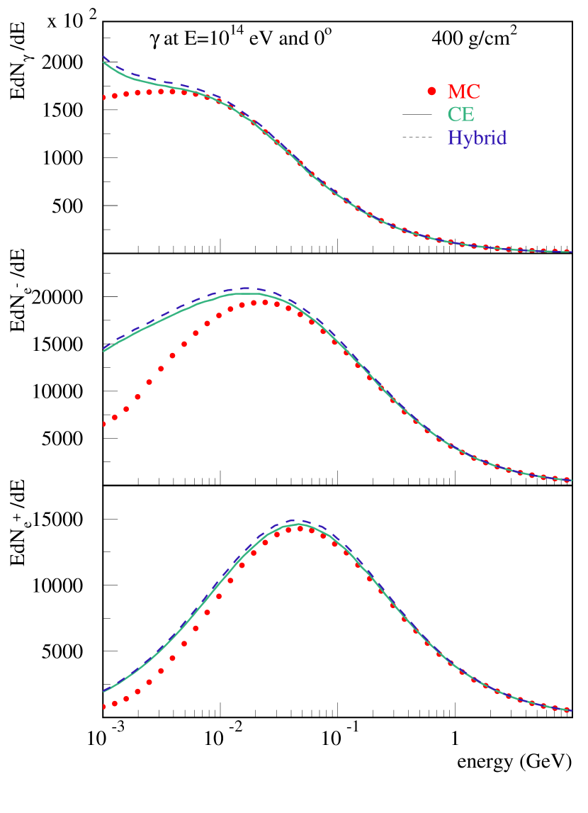
Figure 3: Average longitudinal shower size profiles of charged particles for $E_{\min}^{{\rm e/m}}=$1 MeV (top left panel) and $E_{\min}^{{\rm e/m}}=$1000 MeV (bottom left panel). Particle energy spectra of photons, electrons, and positrons are given in the right panel. All curves are calculated for photon-initiated e/m showers using both hybrid (dashed line), pure MC (points) and cascade equation (solid line) approaches.

While for a large cutoff energy, for example 1000 MeV, the agreement between the different methods is good we notice systematically larger particle numbers in the hybrid and numerical calculations for $E_{\min}^{{\rm e/m}}=$1 MeV. The corresponding difference is clearly visible in the particle energy spectra and is related to spatial effects in the shower development. Low energy electrons (positrons) undergo significant angular deflections due mainly to multiple Coulomb scattering. In turn low energy bremsstrahlung photons produced by such deflected particles also have significant directional deviations from the initial shower axis. If only the track projected to the shower axis is considered, this leads to an apparently faster absorption of low energy particles (higher interaction rate and ionization energy loss) compared to that expected for particles traveling along the shower axis only (see also discussion in [43]). Although a full account of this effect requires a three-dimensional treatment of the particle cascade at MeV energies a reasonable improvement can be achieved by introducing an “average angular deflection”. As the effect is only important for low energy leptons which anyway lose their energy quite fast we may estimate the corresponding average scattering angle of an electron (positron) as

$$\langle\theta^{2}\rangle\sim\frac{E_{s}^{2}}{E^{2}}L\!(E),$$ (16)

where $E_{s}\simeq 21$ MeV and $L\!(E)$ is the average travel distance of an electron of energy $E$ in units of radiation length. With $L\!(E)\simeq E/E_{{\rm crit}}$ and $E_{{\rm crit}}\simeq 81$ MeV, we have

$$\langle\theta^{2}\rangle\sim\frac{E_{s}^{2}}{E\,E_{{\rm crit}}}\,.$$ (17)

For numerical applications, expression (17) has to be modified to satisfy the boundary condition $\theta\leq\pi/2$. In the following we chose the ansatz

$$\langle\theta^{2}\rangle=\left(\frac{\pi}{2}\right)^{2}\left[1-\exp\!\left(-\frac{E_{e^{\pm}}^{{\rm eff}}}{E}\right)\right],$$ (18)

which reduces to the functional form of (17) for large $E$ and approaches $(\pi/2)^{2}$ in the small $E$ limit. The same kind of formula is used for photons but with a different parameter $E_{\gamma}^{{\rm eff}}$, as photons themselves do not undergo multiple scattering. Good agreement between fully three-dimensional MC simulations and cascade equation calculations is obtained for $E_{e^{\pm}}^{{\rm eff}}=9.5\cdot 10^{-4}$ GeV and $E_{\gamma}^{{\rm eff}}=5\cdot 10^{-4}$ GeV. This is shown in Fig. 4 where the shower size profiles and energy spectra of the two approaches are compared for e/m showers of $10^{14}$ eV and $10^{16}$ eV.

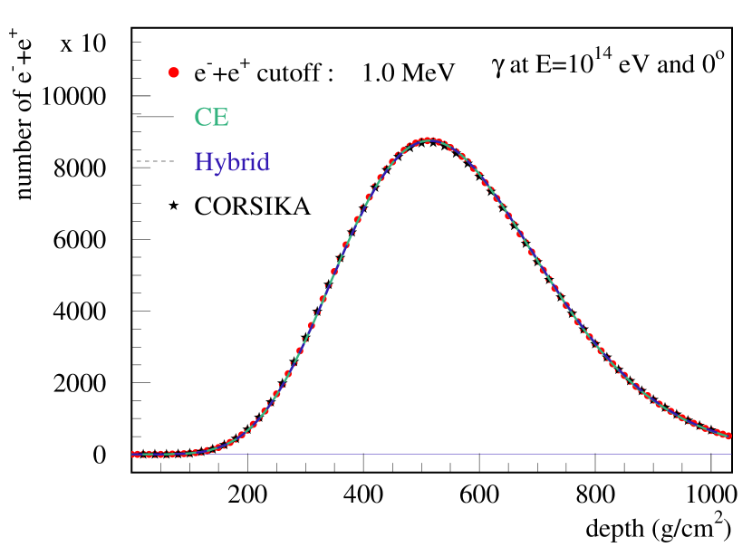
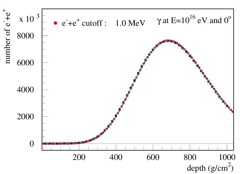
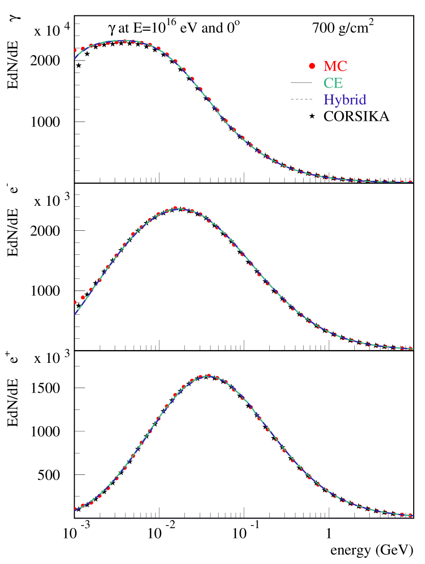
Figure 4: Left panel: Average longitudinal shower size profiles of charged particles for $10^{14}$ eV (top) and $10^{16}$ eV (bottom) photon-initiated showers and $E_{\min}^{{\rm e/m}}=1$ MeV. Right panel: Particle energy spectra at $X=700$ g/cm². Shown are the results of MC simulations with conex and corsika and of the hybrid and cascade equation schemes. Here an “average angular deflection” is used in the numerical and hybrid schemes.

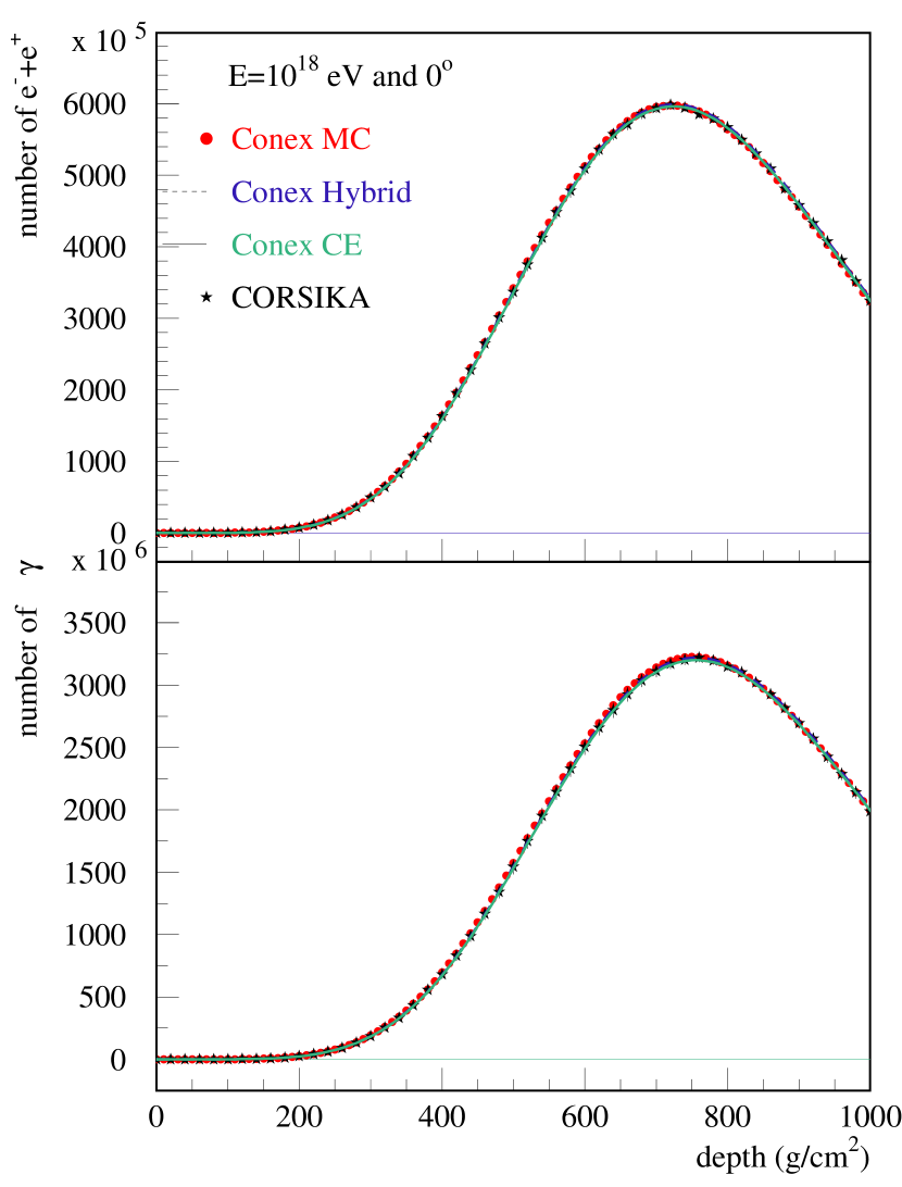
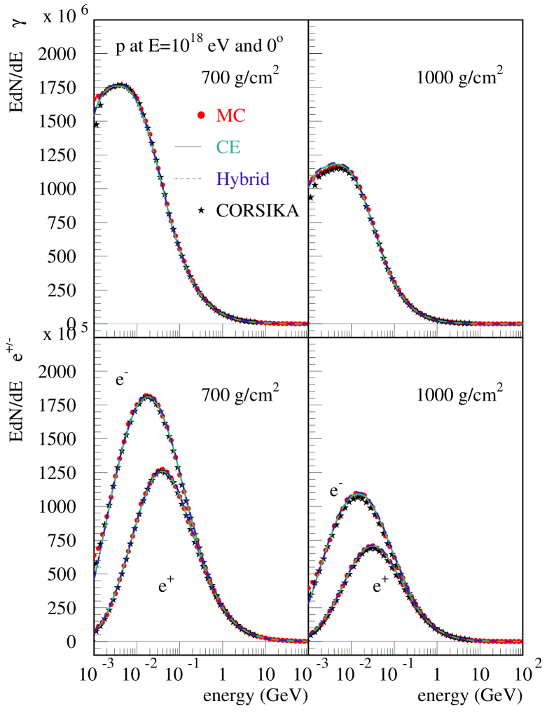
Figure 5: Left panel: Average longitudinal profiles of charged particles and photons of energies above 1 MeV for proton-initiated vertical showers of $E_{0}=10^{18}$ eV. Right panel: Particle energy spectra of photons, electrons, and positrons for the atm. depths $X=700$ and 1000 g/cm². Shown are the results from the hybrid calculation (dashed line), pure MC simulation (points), and numerical cascade Eqs. solution (full line). In addition corsika predictions are given by stars.

After having shown that both hadronic and e/m showers can be well described by the presented cascade equations and the corresponding hybrid simulation scheme, we test the coupling between the e/m and hadronic shower components. In Fig. 5 we compare both longitudinal profiles and energy spectra of e/m particles for vertical proton-induced showers of $10^{18}$ eV. Very good agreement is found between the results of the different calculation methods and also with the corsika predictions. The simulations were performed using qgsjet 01 as high-energy interaction model and gheisha for hadronic interactions at low energy.

3.3 Energy deposit

The longitudinal profile of simulated EAS depends on the e/m low-energy cut-off $E_{\rm min}^{\rm e/m}$ used in the calculation (in this work 1 MeV). Lowering this threshold to, for example, 50 keV would increase the number of charged particles at the shower maximum by a few percent [44]. In the case of the photon number, the dependence of the simulation results on the low-energy cut-off is much stronger. In fact, the number of photons diverges if the simulation cut-off is set to 0. Problems of this kind can be avoided if, instead of the secondary particle profile, the ionization energy deposit profile of showers is considered. Another advantage of the energy deposit profile is its direct relation to the light curve measured in air fluorescence experiments. Current measurements support the theoretical expectation that the fluorescence yield is proportional to the ionization energy deposit [45].

Therefore, the hybrid simulation scheme implemented in conex has been extended to also allow the calculation of energy deposit profiles as described below.

The calculation of the energy deposit profile in the MC part of conex is very similar to that in corsika, see [46]. The deposited ionization energy is counted for each particle and traversed slant depth bin. If a particle reaches the cut-off energy of the calculation, depending on the particle type, either all its energy or a part of it is assumed to be deposited locally. For example, a positron is expected to annihilate in the end and, therefore, all its energy plus electron mass are assumed to be deposited. The different energy contributions taken to be deposited locally are given in Table 1.

Table 1: Energy deposited locally for particles with $E_{\rm kin}<E_{\rm min}$ ($\mathrm{m_{e}}$ denotes the electron mass and $m_{N}$ is the nucleon mass).

particle	$\gamma$	$e^{-}$	$e^{+}$	$\mu^{\pm}$	$\nu$	protons	neutrons	$\pi^{\pm}$,$\mathrm{K^{\pm}}$
energy deposit	$E_{\rm tot}$	$E_{\rm kin}$	$E_{\rm tot}+m_{e}$	$E_{\rm tot}/3$	0	$E_{\rm kin}$	0	$E_{\rm tot}/4$

particle	$\mathrm{K^{0}}$	baryons	anti-baryons	nuclei	anti-nuclei
energy deposit	$E_{\rm tot}/2$	$E_{\rm tot}-m_{N}$	$E_{\rm tot}+m_{N}$	$E_{\rm tot}-A\cdot m_{N}$	$E_{\rm tot}+A\cdot m_{N}$

Solving cascade equations numerically one can calculate the energy deposit of particles with $E>E_{\rm min}$ explicitly. In addition the number of newly created particles at each step in atmospheric depth is given by the source functions. However, the energy carried by particles falling below the cut-off energy threshold and that of neutrinos is not directly calculated.

For the e/m cascade equations, the total energy deposit per slant depth bin can be estimated from energy conservation. The deposited energy follows from the difference between the total kinetic energy at slant depths $X_{m}$ and $X_{m-1}$, including a correction for positrons similar to the MC treatment

$$E_{\rm dep}^{\rm e/m}(X_{m}) = \sum_{i=i_{\rm min}}^{i_{\rm max}}\left(E_{i}^{\mathrm{e/m}}\sum_{a=e^{\pm},\gamma}l_{a}^{i}(X_{m})+2\,m_{\mathrm{e}}\;l_{e^{+}}^{i}(X_{m})\right)$$ (19)

$$-\sum_{i=i_{min}}^{i_{max}}\left(E_{i}^{\mathrm{e/m}}\sum_{a=e^{\pm},\gamma}l_{a}^{i}(X_{m-1})+2\,m_{\mathrm{e}}\;l_{e^{+}}^{i}(X_{m-1})\right),$$

where $m_{e}$ is electron mass.

A similar energy conservation-based method can be applied to the hadronic shower component, however, the deposited energy and the energy going into neutrino production have to be distinguished. Since we know the ionization energy deposited by hadrons and can calculate the number of neutrinos produced within a given slant depth bin, we can obtain the energy of all the particles falling below the low-energy threshold from

$$E_{\rm cut}(X_{m})=E_{\rm bal}(X_{m})-E_{\rm ion}(X_{m})-E_{\nu}(X_{m}),$$ (20)

where

$$E_{\rm bal}(X_{m}) = \sum_{i=i_{min}}^{i_{max}}\left(E_{i}^{\mathrm{had}}\sum_{a}h_{a}^{i}(X_{m})+\sum_{a}m_{a}\;h_{a}^{i}(X_{m})\right)$$ (21)

$$- \sum_{i=i_{min}}^{i_{max}}\left(E_{i}^{\mathrm{had}}\sum_{a}h_{a}^{i}(X_{m-1})+\sum_{a}m_{a}\;h_{a}^{i}(X_{m-1})\right)$$

$$E_{\rm ion}(X_{m}) = \sum_{i=i_{min}}^{i_{max}}\sum_{a}\,h_{a}^{i}(X_{m-1})\>\left(1-\exp\left[-\frac{\beta_{a}^{{\rm ion}}(E_{i}^{{\rm had}})}{E_{i}^{{\rm had}}-E_{i-1}^{{\rm had}}}\Delta X\right]\right)$$ (22)

$$\times \exp\!\left[-\frac{1-W_{a\rightarrow a}^{ii}}{\lambda_{a}(E_{i}^{{\rm had}})}\Delta X-\frac{m_{a}\left|L(X_{m})-L(X_{m-1})\right|}{c\tau_{a}^{(0)}E_{i}^{{\rm had}}}\right]$$

$$E_{\nu}(X_{m}) = \int_{X_{m-1}}^{X_{m}}\!dX^{\prime}\sum_{d}\sum_{j=i+1}^{i_{\max}}\,h_{d}^{j}(X^{\prime})\,D_{d\rightarrow\nu}^{ji}\frac{m_{d}/(c\tau_{d}^{(0)})}{\rho_{{\rm air}}(X^{\prime})}.$$ (23)

To account for the fact that only a part of the energy carried by hadrons falling below the low-energy threshold is deposited as ionization energy, a factor $f_{\mathrm{had}/\mu}=0.45$ is introduced [47]. Thus, the energy deposit for the hadronic part of the system of cascade Eqs. is given by

$$E_{\rm dep}^{\rm had}(X_{m})=E_{\rm ion}(X_{m})+f_{\mathrm{had}/\mu}\;E_{\rm cut}(X_{m}).$$ (24)

Summing the different contributions, the longitudinal energy deposit profile can be calculated. A comparison of the results of different calculation methods within conex with corsika predictions is shown in Fig. 6 (top panel). Good agreement is found.

An interesting consistency check of the energy deposit calculation scheme is the investigation of the dependence of corresponding results on the low-energy threshold used in the e/m cascade Eqs. In Fig. 6 (bottom panel), the mean longitudinal energy deposit profiles of iron-initiated showers of $\theta=60^{\circ}$ and $E=10^{19}$ eV are shown for different low-energy thresholds. The profiles are independent of this threshold over a wide energy range – the approximation of local energy deposit breaks down only for a threshold energy of 100 MeV and higher.

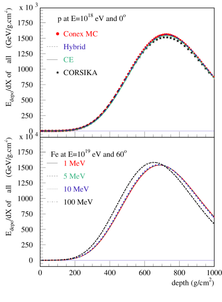
Figure 6: Upper panel: Average longitudinal energy deposit profile for vertical proton-initiated showers of $10^{18}$ eV. The results obtained with the e/m energy cutoff $E_{\rm min}^{{\rm e/m}}=1$ MeV, using hybrid (dashed line), MC (points), or numerical approaches (full line), are compared to corsika predictions (stars). Lower panel: Energy deposit profiles for $10^{19}$ eV inclined ($\theta=60^{{\rm o}}$) iron-initiated showers for the e/m energy cutoff $E_{\min}^{{\rm e/m}}=$1 (full line), 5 (dashed line), 10 (dotted line) and 100 MeV (dashed-dotted line).

3.4 Shower fluctuations

So far we have only studied mean shower observables, i.e. ones averaged over many showers. As a proper description of shower fluctuations is of central importance for the analysis of experimental data, we will also discuss the treatment of shower fluctuations.

Running conex in hybrid mode allows us to benefit from the fast numerical solution of cascade Eqs. and, at the same time, to obtain a good description of shower-to-shower fluctuations. Here, the key parameter of the method is the energy threshold that separates the explicit MC simulation from the application of cascade Eqs. By default, this energy threshold is set to $E_{\rm thr}=0.01\cdot E_{0}$ for all particles in conex. In principle, it can be chosen differently for e/m and hadronic particles to further reduce the simulation time needed for high-energy showers.

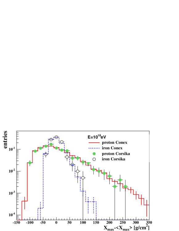
Figure 7: Fluctuations of the shower maximum depth $\mathrm{X}_{\mathrm{max}}$around the mean shower maximum depth $\left\langle\mathrm{X}_{\mathrm{max}}\right\rangle$ for a primary energy of $10^{18}$eV for proton and iron-initiated showers simulated with conex (lines) and compared with corsika results (points).

In Fig. 7 the distribution of the depth of shower maximum is shown for proton- and iron-initiated showers. Within the statistical uncertainties, the conex results agree very well with that obtained with corsika MC simulations. Not only the fluctuations but also the mean depth of shower maximum obtained with the two codes are the same (not shown).

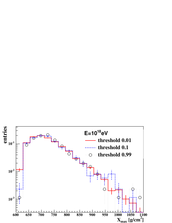
Figure 8: Fluctuations of the shower maximum depth $\mathrm{X}_{\mathrm{max}}$ for $10^{18}$eV proton-initiated showers simulated with conex for three different energy thresholds $E_{\rm thr}/E_{0}=0.01$, 0.1, 0.99.

The dependence of the simulated fluctuations on the energy threshold is shown in Fig. 8. Even a threshold as large as $E_{\rm thr}=0.99\cdot E_{0}$ is sufficient to reproduce almost the full $X_{\rm max}$ distribution. This comparison demonstrates that the fluctuations of particle production in the first interaction of such high-energy showers determine almost the entire shower profile.

4 Summary

We have developed a fast and efficient one-dimensional hybrid simulation scheme for ultra-high energy air showers. It combines explicit MC simulation of high-energy particle interaction, propagation and decay with the numerical solution of a system of cascade equations for calculating the low-energy part of the particle cascade.

The presented hybrid simulation scheme is implemented in the code conex. Several high- and low-energy hadronic interaction models are available within conex to study theoretical predictions and the model-dependence of data analyses.

All relevant interaction and decay processes are considered in both the MC and the cascade equation parts of conex. These processes also include muon pair production and photonuclear interactions of muons. At ultra-high energy, the LPM effect and possible e/m preshowering in the geo-magnetic field are simulated.

The hybrid simulation scheme has been extended to include the simultaneous calculation of both shower size profiles of various particles and the generation of ionization energy deposit profiles. The latter are independent of the low-energy cut-off that has to be applied in all shower simulations. Knowing both the shower size profile (with an arbitrary low-energy cut-off) and the energy deposit profile allows us to simulate directly the fluorescence and Cherenkov light signal of air showers. Together with the fully three-dimensional implementation of the shower axis geometry, this makes conex ideally suited for event simulation and data analysis of fluorescence light experiments such as HiRes [48], Auger [49], TA [50], and EUSO [51].

In developing conex, particular emphasis is put on the accuracy and reliability of the shower simulation to make the code directly applicable to data analysis of air shower experiments. Extensive comparisons with corsika simulations show that all shower distributions agree very well. Both mean shower profiles and energy distributions as well as their fluctuations were compared, only a small fraction of which could be shown in this paper.

In a forthcoming work we will study the influence of different hadronic interaction models on air shower predictions. In particular we will investigate the total calorimetric energy deposited by a shower in air. First results of this work have been presented in [52].

5 Appendix

5.1 Geometry

Using a one-dimensional treatment of EAS development, a given shower trajectory may be characterized by a single parameter - its distance to the center of the Earth $O$: $R_{\perp}^{T}=\left|P_{l}^{T}O\right|$ - see Fig. 9, where $P_{l}^{T}$ is the lowest trajectory point.

Figure 9: Geometry for defining the shower trajectory accounting for the curvature of the Earth.

In case the observer is positioned at some height $h_{{\rm obs}}$ above sea level and $R_{{\rm Earth}}+h_{{\rm obs}}>R_{\perp}^{T}$ ($R_{{\rm Earth}}$ being the Earth radius) the observed shower inclination is

$$\theta=\arcsin\frac{R_{\perp}^{T}}{R_{{\rm Earth}}+h_{{\rm obs}}}.$$ (25)

The position of a particle moving along a given trajectory may be then characterized by its local azimuthal angle $\theta_{P}^{T}$ with respect to the vertical direction, or alternatively, by its height $H_{P}^{T}$, or by the distance $L_{P}^{T}=\left|P_{l}^{T}P\right|$ to the lowest trajectory point

$$H_{P}^{T}=\frac{R_{\perp}^{T}}{\sin\theta_{P}^{T}}$$ (26)

$$L_{P}^{T}=\frac{R_{\perp}^{T}}{\cos\theta_{P}^{T}}.$$ (27)

For the solution of cascade equations, it is more convenient to use instead the slant grammage $X_{P}^{T}$, i.e. the integral over the atmospheric density $\rho_{{\rm air}}(h)$ along the trajectory $T$ from the point $P$ to infinity

$$X_{P}^{T}=\int_{L_{P}^{T}}^{\infty}\!dl^{\prime}\;\rho_{{\rm air}}\left(H(l^{\prime})\right),$$ (28)

and characterize an arbitrary particle position by two variables, $R_{\perp}^{T}$ and $X$.

5.2 Numerical treatment of hadronic cascade equations

In order to reduce the problem to the solution of a system of ordinary differential equations, we perform a discretization of particle energy spectra. Introducing an energy binning as $E_{i}^{{\rm had}}=E_{\min}^{{\rm had}}\;C^{i-1}$, $C=\,10^{1/d_{E}}$ ($E_{\min}^{{\rm had}}=1$ GeV, $d_{E}=10\div 30$) and replacing the smooth particle spectra $h_{a}\!(E,X)$ by discrete contributions $h_{a}^{i}\!(X)$ of representative particles of energies $E_{i}^{{\rm had}}$ ($i=1,...,i_{\max}$) we may get instead of (1)

$$\frac{dh_{a}^{i}(X)}{dX} = -h_{a}^{i}(X)\left[\frac{1}{\lambda_{a}(E_{i}^{{\rm had}})}+\left|\frac{dL}{dX}\right|\frac{m_{a}}{c\,\tau_{a}^{(0)}\>E_{i}^{{\rm had}}}+\frac{\beta_{a}^{{\rm ion}}(E_{i}^{{\rm had}})}{E_{i}^{\mathrm{had}}-E_{i-1}^{\mathrm{had}}}\right]$$ (29)

$$+\sum_{d}\sum_{j=i}^{i_{\max}}\;h_{d}^{j}(X)\;\left[\frac{W_{d\rightarrow a}^{ji}}{\lambda_{d}(E_{j}^{{\rm had}})}+D_{d\rightarrow a}^{ji}\frac{m_{d}/(c\,\tau_{d}^{(0)})}{E_{j}^{{\rm had}}\;\rho_{{\rm air}}(X)}\right]$$

$$+h_{a}^{i+1}(X)\,\frac{\beta_{a}^{{\rm ion}}(E_{i+1}^{{\rm had}})}{E_{i+1}^{\mathrm{had}}-E_{i}^{\mathrm{had}}}+S_{ai}^{{\rm had}}(X),$$

where we used (4), replaced the integral over parent particle energies $\int\!dE^{\prime}$ by the discrete sum $\sum_{j}$, introduced the discretized source term $S_{ai}^{{\rm had}}(X)$ and the discrete interaction (decay) spectra $W_{d\rightarrow a}^{ij}$ ($D_{d\rightarrow a}^{ij}$) via

$$S_{ai}^{{\rm had}}(X) = \int_{\max\left[E_{i-1}^{{\rm had}},E_{\min}^{{\rm had}}\right]}^{E_{i}^{{\rm had}}}\!dE^{\prime}\;S_{a}^{{\rm had}}(E^{\prime},X)\;K(E^{\prime}/E_{i}^{{\rm had}})$$ (30)

$$+\int_{E_{i}^{{\rm had}}}^{\min\left[E_{i+1}^{{\rm had}},E_{{\rm thr}}\right]}\!dE^{\prime}\;S_{a}^{{\rm had}}(E^{\prime},X)\,\left[1-K(E^{\prime}/E_{i+1}^{{\rm had}})\right]$$

$$W_{d\rightarrow a}^{ij} = \int_{\max\left[E_{i-1}^{{\rm had}},E_{\min}^{{\rm had}}\right]}^{E_{i}^{{\rm had}}}\!dE^{\prime}\;W_{d\rightarrow a}(E^{\prime},E_{j}^{{\rm had}})\;K(E^{\prime}/E_{i}^{{\rm had}})$$ (31)

$$+\int_{E_{i}^{{\rm had}}}^{\min\left[E_{i+1}^{{\rm had}},E_{{\rm thr}}\right]}\!dE^{\prime}\;W_{d\rightarrow a}(E^{\prime},E_{j}^{{\rm had}})\,\left[1-K(E^{\prime}/E_{i+1}^{{\rm had}})\right],$$

and the discrete energy loss term via :

$$-\beta_{a}^{{\rm ion}}(E_{i}^{{\rm had}})\>\frac{h_{a}^{i}(X)}{E_{i}^{\mathrm{had}}-E_{i-1}^{\mathrm{had}}}+\beta_{a}^{{\rm ion}}(E_{i+1}^{{\rm had}})\>\frac{h_{a}^{i+1}(X)}{E_{i+1}^{\mathrm{had}}-E_{i}^{\mathrm{had}}}\,.$$

Here the condition of both energy and particle number conservation gives

$$K(\varepsilon)=\frac{C\>\varepsilon-1}{C-1}\,.$$ (32)

The solution of the homogeneous part of Eq. (29) is

$$h_{a}^{i}(X)=h_{a}^{i}(X_{0})\>\exp\!\left[-\left(\frac{1-W_{a\rightarrow a}^{ii}}{\lambda_{a}(E_{i}^{{\rm had}})}+\frac{\beta_{a}^{{\rm ion}}(E_{i}^{{\rm had}})}{E_{i}^{{\rm had}}-E_{i-1}^{{\rm had}}}\right)(X-X_{0})-\frac{m_{a}\left|L(X)-L(X_{0})\right|}{c\tau_{a}^{(0)}E_{i}^{{\rm had}}}\right].$$ (33)

Correspondingly the solution of the full equation can be obtained in an iterative way

$$h_{a}^{i}(X) = h_{a}^{i}(X_{0})\>\exp\!\left[-\left(\frac{1-W_{a\rightarrow a}^{ii}}{\lambda_{a}(E_{i}^{{\rm had}})}+\frac{\beta_{a}^{{\rm ion}}(E_{i}^{{\rm had}})}{E_{i}^{{\rm had}}-E_{i-1}^{{\rm had}}}\right)(X-X_{0})-\frac{m_{a}\left|L(X)-L(X_{0})\right|}{c\tau_{a}^{(0)}E_{i}^{{\rm had}}}\right]$$ (34)

$$+\int_{X_{0}}^{X}\!dX^{\prime}\left\{\sum_{d}\sum_{j=i+1}^{i_{\max}}h_{d}^{j}(X^{\prime})\,\left[\frac{W_{d\rightarrow a}^{ji}}{\lambda_{d}(E_{j}^{{\rm had}})}+D_{d\rightarrow a}^{ji}\frac{m_{d}/(c\tau_{d}^{(0)})}{E_{j}^{{\rm had}}\rho_{{\rm air}}(X^{\prime})}\right]\right.$$

$$\left.+h_{a}^{i+1}(X^{\prime})\frac{\beta_{a}^{{\rm ion}}(E_{i+1}^{{\rm had}})}{E_{i+1}^{\mathrm{had}}-E_{i}^{\mathrm{had}}}+S_{ai}^{{\rm had}}(X^{\prime})\right\}$$

$$\times\exp\!\left[-\left(\frac{1-W_{a\rightarrow a}^{ii}}{\lambda_{a}(E_{i}^{{\rm had}})}+\frac{\beta_{a}^{{\rm ion}}(E_{i}^{{\rm had}})}{E_{i}^{{\rm had}}-E_{i-1}^{{\rm had}}}\right)(X-X^{\prime})-\frac{m_{a}\left|L(X)-L(X^{\prime})\right|}{c\tau_{a}^{(0)}E_{i}^{{\rm had}}}\right].$$

Discretizing depth positions as $X_{m}=m\,\Delta\!X$, $m=1,...,m_{\max}$, $X_{m_{\max}}$ corresponding to the observation level for the given shower trajectory, the formulas (33-34) can be used to calculate spectra of different hadrons at all depths $X_{m}$, starting from the initial condition $h_{a}^{i}(X_{m})$ for $m=1$, calculating first $h_{a}^{i_{\max}}(X_{m+1})$, using Eq. (33), and $h_{a}^{i_{\max}-1}(X_{m+1})$, $h_{a}^{i_{\max}-2}(X_{m+1})$, … , $h_{a}^{1}(X_{m+1})$, using Eq. (34), etc. for $m=2,...,m_{\max}$. The depth integral in Eq. (34) is taken using the Simpson formula; particle spectra values $h_{a}^{i}(X_{m+1/2})$ at mids of the bins $X_{m+1/2}=(X_{m}+X_{m+1})/2$ are obtained via a logarithmic interpolation between previously calculated $h_{a}^{i}(X_{m})$, $h_{a}^{i}(X_{m+1})$.

As for neutral pions, we assume them to decay at the place, calculate the number of $\pi^{0}$s produced at depth $X_{m}$ as

$$h_{\pi^{0}}^{i}(X_{m}) = \int_{X_{m-1}}^{X_{m}}\!dX^{\prime}\sum_{d}\sum_{j=i+1}^{i_{\max}}\,h_{d}^{j}(X^{\prime})$$ (35)

$$\times\left[\frac{W_{d\rightarrow\pi^{0}}^{ji}}{\lambda_{d}(E_{j}^{{\rm had}})}+D_{d\rightarrow\pi^{0}}^{ji}\frac{m_{d}/(c\,\tau_{d}^{(0)})}{E_{j}^{{\rm had}}\;\rho_{{\rm air}}(X^{\prime})}\right]+\int_{X_{m-1}}^{X_{m}}\!dX^{\prime}\>S_{\pi^{0}i}^{{\rm had}}(X^{\prime})$$

and add photons resulting from $\pi^{0}$ decay to the e/m source function.

5.3 Numerical treatment of e/m cascade equations

To reduce the problem to the solution of a system of ordinary differential equations we again, like in case of hadron cascade, discretize particle energy spectra $l_{a}\!(E,X)$ using an energy grid $E_{i}^{{\rm e/m}}=E_{\min}^{{\rm e/m}}\,C^{i-1}$ ($E_{\min}^{{\rm e/m}}=0.1\div 1$ MeV), replace the integral over parent particle energy $E^{\prime}$ in (6-8) by a sum over discrete energies, and discretize the source term $S_{a}^{{\rm e/m}}\!(E,X)$ and the differential energy spectra $W_{d\rightarrow a}(E^{\prime},E)$ according to (30-31) (with $E_{i}^{{\rm had}}$, $E_{\min}^{{\rm had}}$, $S_{a}^{{\rm had}}\!(E^{\prime},X)$ being replaced by $E_{i}^{{\rm e/m}}$, $E_{\min}^{{\rm e/m}}$, $S_{a}^{{\rm e/m}}\!(E^{\prime},X)$). Then Eqs. (6-8) are transformed to

$$\frac{dl_{a}^{i}(X)}{dX}=\sum_{d}\sum_{j=i}^{i_{\max}}\bar{W}_{d\rightarrow a}^{ji}\;l_{d}^{j}(X)+S_{ai}^{{\rm e/m}}\!(X),$$ (36)

where we replaced the continuous energy loss term $\frac{\partial}{\partial E}\left(\beta_{e^{\pm}}^{{\rm ion}}(E)l_{e^{\pm}}(E,X)\right)$ by

$$-\beta_{e^{\pm}}^{{\rm ion}}\!(E_{i}^{{\rm e/m}})\;\frac{l_{e^{\pm}}^{i}\!(X)}{E_{i}^{{\rm e/m}}-E_{i-1}^{{\rm e/m}}}+\beta_{e^{\pm}}^{{\rm ion}}\!(E_{i+1}^{{\rm e/m}})\;\frac{l_{e^{\pm}}^{i+1}\!(X)}{E_{i+1}^{{\rm e/m}}-E_{i}^{{\rm e/m}}}$$

and included the two terms, together with the interaction cross sections, into the discrete particle production spectra $\bar{W}_{d\rightarrow a}^{ji}$, defined as follows

$$\bar{W}_{e^{\pm}\rightarrow e^{\pm}}^{ii}=W_{e^{\pm}\rightarrow e^{\pm}}^{ii}-\sigma_{e^{\pm}}\!(E_{i}^{{\rm e/m}})-\frac{\beta_{e^{\pm}}^{{\rm ion}}\!(E_{i}^{{\rm e/m}})}{(C-1)E_{i}^{{\rm e/m}}}$$ (37)

$$\bar{W}_{e^{\pm}\rightarrow e^{\pm}}^{i,i-1}=W_{e^{\pm}\rightarrow e^{\pm}}^{i,i-1}+\frac{\beta_{e^{\pm}}^{{\rm ion}}\!(E_{i}^{{\rm e/m}})}{(C-1)E_{i}^{{\rm e/m}}}$$ (38)

$$\bar{W}_{\gamma\rightarrow\gamma}^{ii}=W_{\gamma\rightarrow\gamma}^{ii}-\sigma_{\gamma}\!(E_{i}^{{\rm e/m}}),$$ (39)

and $\bar{W}_{d\rightarrow a}^{ij}=W_{d\rightarrow a}^{ij}$ for all other combinations of $i$, $j$, $a$, $d$.

It is worth verifying that all elements of the matrixes $\bar{W}_{d\rightarrow a}^{ij}$ are free of singularities. Indeed, singular terms appear in $\sigma_{e^{\pm}}^{{\rm brems}}\!(E_{i}^{{\rm e/m}})=\int_{0}^{E_{i}^{{\rm e/m}}}\!dE^{\prime}\;W_{e^{-}\rightarrow e^{-}}^{{\rm brems}}\!(E_{i}^{{\rm e/m}},E^{\prime})$ and in $W_{e^{\pm}\rightarrow e^{\pm}}^{ii}$ (defined by Eq. (31)) due to the characteristic $1/(E-E^{\prime})$ dependence of $W_{e^{-}\rightarrow e^{-}}^{{\rm brems}}\!(E,E^{\prime})$. Nevertheless, in $\bar{W}_{e^{\pm}\rightarrow e^{\pm}}^{ii}$ defined by Eq. (37) the corresponding singularities are canceled against each other

$$\bar{W}_{e^{\pm}\rightarrow e^{\pm}}^{({\rm brems})ii} = W_{e^{\pm}\rightarrow e^{\pm}}^{({\rm brems})ii}-\sigma_{e^{\pm}}^{{\rm brems}}\!(E_{i}^{{\rm e/m}})$$ (42)

$$= \int_{E_{i-1}^{{\rm e/m}}}^{E_{i}^{{\rm e/m}}}\!dE^{\prime}\;W_{e^{-}\rightarrow e^{-}}^{{\rm brems}}\!(E_{i}^{{\rm e/m}},E^{\prime})\;\frac{C\>E^{\prime}/E_{i}^{{\rm e/m}}-1}{C-1}$$

$$-\int_{0}^{E_{i}^{{\rm e/m}}}\!dE^{\prime}\;W_{e^{-}\rightarrow e^{-}}^{{\rm brems}}\!(E_{i}^{{\rm e/m}},E^{\prime})$$

$$= -\frac{C}{E_{i}^{{\rm e/m}}\>(C-1)}\int_{E_{i-1}^{{\rm e/m}}}^{E_{i}^{{\rm e/m}}}\!dE^{\prime}\;(E_{i}^{{\rm e/m}}-E^{\prime})\;W_{e^{-}\rightarrow e^{-}}^{{\rm brems}}\!(E_{i}^{{\rm e/m}},E^{\prime})$$

$$-\int_{0}^{E_{i-1}^{{\rm e/m}}}\!dE^{\prime}\;W_{e^{-}\rightarrow e^{-}}^{{\rm brems}}\!(E_{i}^{{\rm e/m}},E^{\prime}),$$

where the last two integrals are finite. Similarly one can check the finiteness of $\bar{W}_{e^{\pm}\rightarrow e^{\pm}}^{i,i-1}$.

To solve the system (36), we first find the solution of the homogeneous equation system

$$\frac{dl_{a}^{i}(X)}{dX}=\sum_{d}\bar{W}_{d\rightarrow a}^{ii}\;l_{d}^{i}(X),$$ (43)

which is given as

$$l_{a}^{i}(X)=\sum_{I=1}^{3}D_{aI}^{i}(X_{0})\;e^{\Lambda_{I}^{i}\>(X-X_{0})}$$ (44)

Here $\Lambda_{I}^{i}$ and $D_{aI}^{i}(X_{0})$ are correspondingly the eigenvalues and eigenvectors of the system of linear algebraic equations obtained by inserting (44) into (43):

$$\Lambda^{i}\;D_{a}^{i}(X_{0})-\sum_{d}\bar{W}_{d\rightarrow a}^{ii}\;D_{d}^{i}(X_{0})=0,$$

with the normalization fixed by the initial conditions at $X=X_{0}$: $\sum_{I=1}^{3}D_{aI}^{i}(X_{0})=l_{a}^{i}(X_{0})$.

Then the solution of the full equation system (36) may be given in a recursive form

$$l_{a}^{i}(X) = \sum_{I=1}^{3}D_{aI}^{i}(X_{0})\>\left[e^{\Lambda_{I}^{i}\>(X-X_{0})}+\sum_{d}F_{Id}^{i}(X_{0})\int_{X_{0}}^{X}\!dX^{\prime}\right.$$ (45)

$$\left.\times\>e^{\Lambda_{I}^{i}\>(X-X^{\prime})}\>\left[S_{di}^{{\rm e/m}}\!(X^{\prime})+\sum_{j=i+1}^{i_{\max}}\sum_{g}\bar{W}_{g\rightarrow d}^{ji}\;l_{g}^{j}(X^{\prime})\right]\right],$$

where the matrix $F_{Id}^{i}$ is inverse with respect to $D_{aI}^{i}$

$$\sum_{I}D_{aI}^{i}(X_{0})\;F_{Id}^{i}(X_{0})=\delta_{a}^{d}\,.$$ (46)

Equations (44-45) can be used to calculate the discrete spectra of e/m particles $l_{a}^{i}(X_{m})$ at all depths $X_{m}$ in the same way as in case of the hadronic cascade.

Acknowledgments

The authors thank Hans-Joachim Drescher, Michael Unger, and Ralf Ulrich for fruitful discussions. N.N.K. acknowledges the financial support of the Russian Foundation for Basic Research (RFBR, grant 05-02-16401). The work of one of the authors, S.O., has been supported in part by the German Ministry for Education and Research (BMBF, Grant 05 CU1VK1/9).

References

- [1] A. M. Hillas, in Proc. 17th Int. Cosmic Ray Conf., v. 8, p. 193, Paris, France, 1981.
- [2] M. Kobal, A. Filipčič, and D. Zavrtanik, Proc. of 26th Int. Cosmic Ray Conf., v. 1, p. 490, Salt Lake City, Utah, USA, 1999.
- [3] M. Risse, D. Heck, J. Knapp, and S. S. Ostapchenko, Proc. 27th Int. Cosmic Ray Conf., v. 2, p. 522, Hamburg, Germany, 2001.
- [4] M. Kobal, Astropart. Phys. 15, 259 (2001).
- [5] L. G. Dedenko, Proc. of 9th Int. Cosmic Ray Conf., v. 1, p. 662, London, UK, 1965.
- [6] M. Hillas, Proc. of 9th Int. Cosmic Ray Conf. v. 1, p. 758, London, UK, 1965.
- [7] G. Bossard, H. J. Drescher, N. N. Kalmykov, S. Ostapchenko, A. I. Pavlov, T. Pierog, E. A. Vishnevskaya, and K. Werner, Phys. Rev. D63, 054030 (2001), hep-ph/0009119.
- [8] N. N. Kalmykov and M. V. Motova, Yadernaya Fizika (Rus) 43, 630 (1986).
- [9] D. Heck, J. Knapp, J. Capdevielle, G. Schatz, and T. Thouw, Wissenschaftliche Berichte FZKA 6019, Forschungszentrum Karlsruhe, 1998.
- [10] T. Stanev and H. P. Vankov, Astropart. Phys. 2, 35 (1994).
- [11] T. K. Gaisser, P. Lipari, and T. Stanev, in Proc. 25th Int. Cosmic Ray Conf., v. 6, p. 281, Durban, South Africa, 1997.
- [12] J. Alvarez-Muniz, R. Engel, T. K. Gaisser, J. A. Ortiz, and T. Stanev, Phys. Rev. D66, 033011 (2002), astro-ph/0205302.
- [13] H. J. Drescher and G. R. Farrar, Phys. Rev. D67, 116001 (2003), astro-ph/0212018.
- [14] W. R. Nelson, H. Hirayama, and D. W. O. Rogers, SLAC-265, Stanford Linear Accelerator Center, 1985.
- [15] H. J. Drescher, M. Hladik, S. Ostapchenko, T. Pierog, and K. Werner, Phys. Rept. 350, 93 (2001), hep-ph/0007198.
- [16] T. Pierog, H. J. Drescher, F. M. Liu, S. Ostapchenko, and K. Werner, Nucl. Phys. A715, 895 (2003), hep-ph/0211202.
- [17] K. Werner, F. M. Liu, S. Ostapchenko, and T. Pierog, J. Phys. G: Nucl. Part. Phys. 30, S211 (2003), hep-ph/0306152.
- [18] N. N. Kalmykov, S. S. Ostapchenko, and A. I. Pavlov, Bull. Russ. Acad. Sci. Phys. 58, 1966 (1994).
- [19] N. N. Kalmykov, S. S. Ostapchenko, and A. I. Pavlov, Nucl. Phys. Proc. Suppl. 52B, 17 (1997).
- [20] S. Ostapchenko, Nucl. Phys. Proc. Suppl. 151 (2006), 143, hep-ph/0412332.
- [21] S. Ostapchenko, Phys. Rev. D (2006), to be published, hep-ph/0505259.
- [22] S. Ostapchenko, to appear in Proc. of INFN Eloisatron Project 44th Workshop on QCD at Cosmic Energies, Erice, Italy, 2004, hep-ph/0501093.
- [23] R. Engel, T. K. Gaisser, T. Stanev, and P. Lipari, Phys. Rev. D46, 5013 (1992).
- [24] R. S. Fletcher, T. K. Gaisser, P. Lipari, and T. Stanev, Phys. Rev. D50, 5710 (1994).
- [25] R. Engel, T. K. Gaisser, P. Lipari, and T. Stanev, Proc. of 26th Int. Cosmic Ray Conf., v. 1, p. 415, Salt Lake City, Utah, USA, 1999.
- [26] H. Fesefeldt, preprint PITHA-85/02, RWTH Aachen, 1985.
- [27] A. B. Migdal, Phys. Rev. 103, 1811 (1956).
- [28] E. Konishi, A. Adachi, N. Takahashi, and A. Misaki, J. Phys. G: Nucl. Part. Phys. 17, 719 (1991).
- [29] D. Heck and J. Knapp, Wissenschaftliche Berichte FZKA 6097, Forschungszentrum Karlsruhe, 1998.
- [30] E. Storm and H. I. Israel, Nuclear Data Tables A7, 565 (1970).
- [31] T. K. Gaisser, Cosmic rays and particle physics, Cambridge Univ. Press, Cambridge, 1990.
- [32] R. M. Sternheimer, M. J. Berger, and S. M. Seltzer, At. Data Nucl. Data Tabl. 30, 261 (1984).
- [33] S. Bottai and L. Perrone, Nucl. Instrum. Meth. A459, 319 (2001), hep-ex/0001018.
- [34] Y. M. Andreev and E. V. Bugaev, Phys. Rev. D55, 1233 (1997).
- [35] L. B. Bezrukov and E. V. Bugaev, Yadernaya Fizika (Rus) 33, 1195 (1981).
- [36] H. Bilokon et al., Nucl. Instrum. Meth. A303, 381 (1991).
- [37] W. Lohmann, R. Kopp, and R. Voss, CERN-85-03, 1985.
- [38] T. Erber, Rev. Mod. Phys. 38, 626 (1966).
- [39] T. Stanev and H. P. Vankov, Phys. Rev. D55, 1365 (1997), astro-ph/9607011.
- [40] H. P. Vankov, N. Inoue, and K. Shinozaki, Phys. Rev. D67, 043002 (2003), astro-ph/0211051.
- [41] P. Homola et al., Comput. Phys. Commun. 173, 71 (2005), astro-ph/0311442.
- [42] T. Stanev, T. K. Gaisser, and F. Halzen, Phys. Rev. D32, 1244 (1985).
- [43] J. Alvarez-Muñiz, E. Marques, R. A. Vazquez, and E. Zas, Phys. Rev. D67, 101303 (2003), astro-ph/0302491.
- [44] F. Nerling, J. Blümer, R. Engel, and M. Risse, Astropart. Phys. 24, 421 (2006).
- [45] AirFly Collab., F. Arciprete et al., Nucl. Phys. Proc. Suppl. 150, 186 (2006).
- [46] M. Risse and D. Heck, Astropart. Phys. 20, 661 (2004), astro-ph/0308158.
- [47] H. M. J. Barbosa, F. Catalani, J. A. Chinellato, and C. Dobrigkeit, Astropart. Phys. 22, 159 (2004), astro-ph/0310234.
- [48] HiRes Collab., R. U. Abbasi et al., Astrophys. J. 622, 910 (2005), astro-ph/0407622.
- [49] Pierre Auger Collab., J. Abraham et al., Nucl. Instrum. Meth. A523, 50 (2004).
- [50] TA Collab., K. Kasahara et al., astro-ph/0511177, 2005.
- [51] EUSO Collab., M. Pallavicini, Nucl. Instrum. Meth. A502, 155 (2003).
- [52] T. Pierog et al., Proc. 29-th Int. Cosmic Ray Conf., v. 7, p. 103, Pune, India, 2005.